Evaporative Fraction as an Indicator of Moisture Condition and Water Stress Status in Semi-Arid Rangeland Ecosystems

 , ,
, ,
Abstract
:
1. Introduction
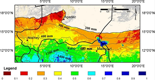
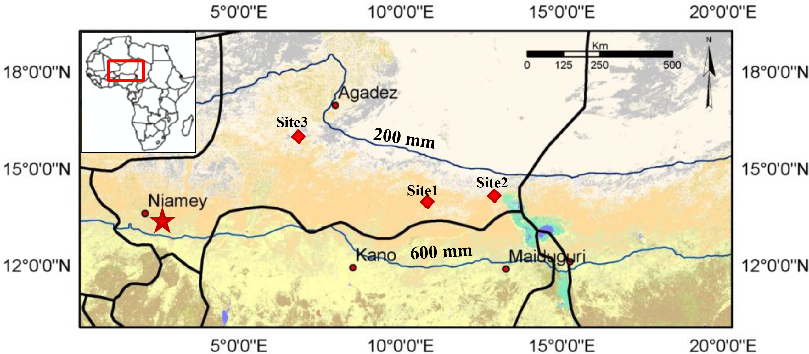
2. Study Area
3. Materials
3.1. Earth Observation Data
3.2. Field Biomass and Flux Measurements
4. Method
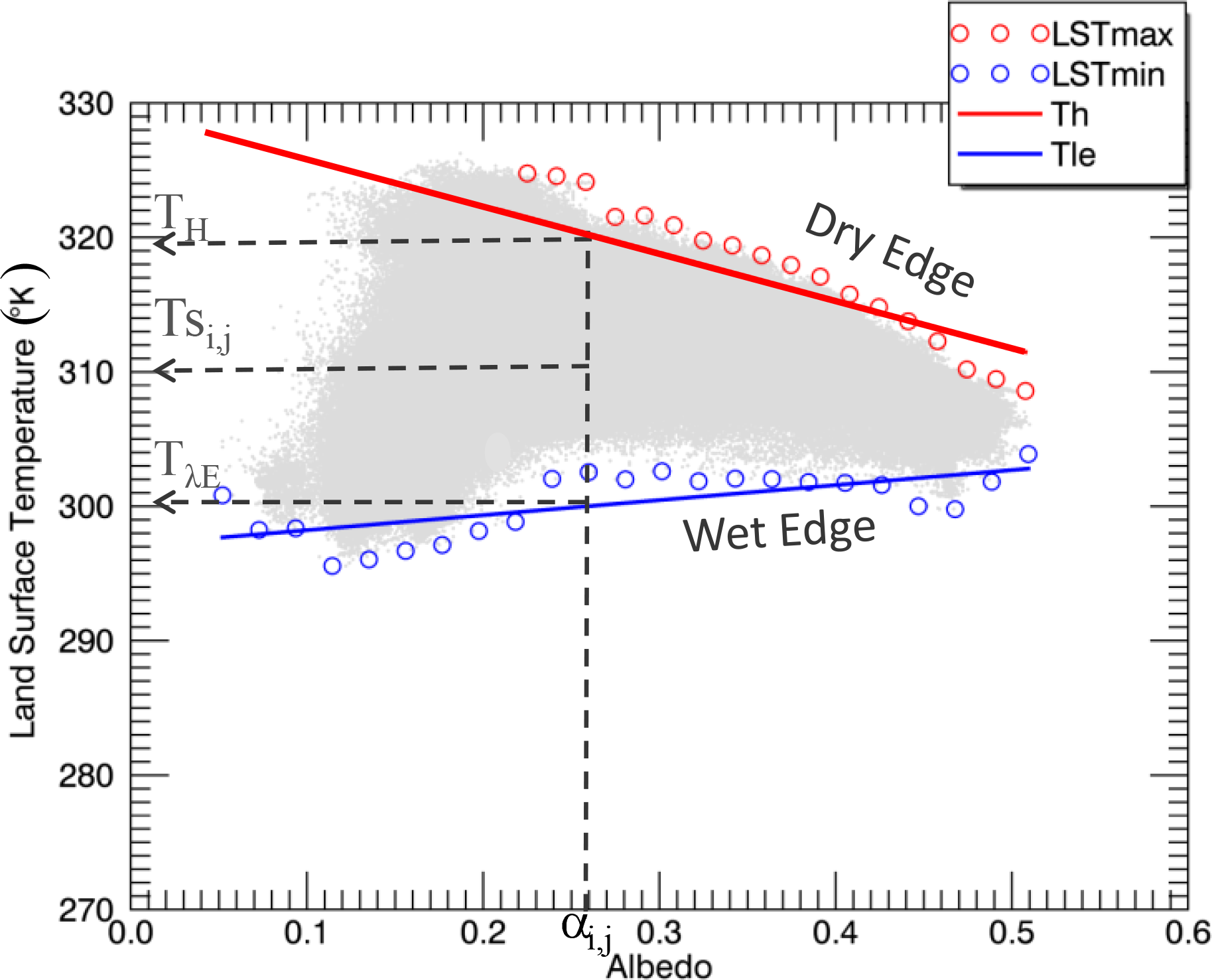
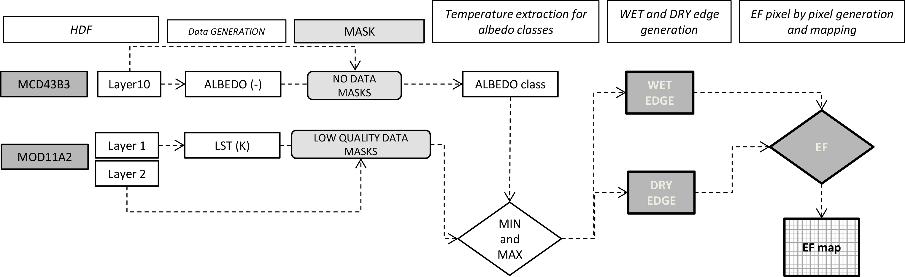
4.1. Estimation of Evaporative Fraction
4.2. Evaluation of the Estimated EF
4.3. Biomass Estimation
5. Results and Discussion
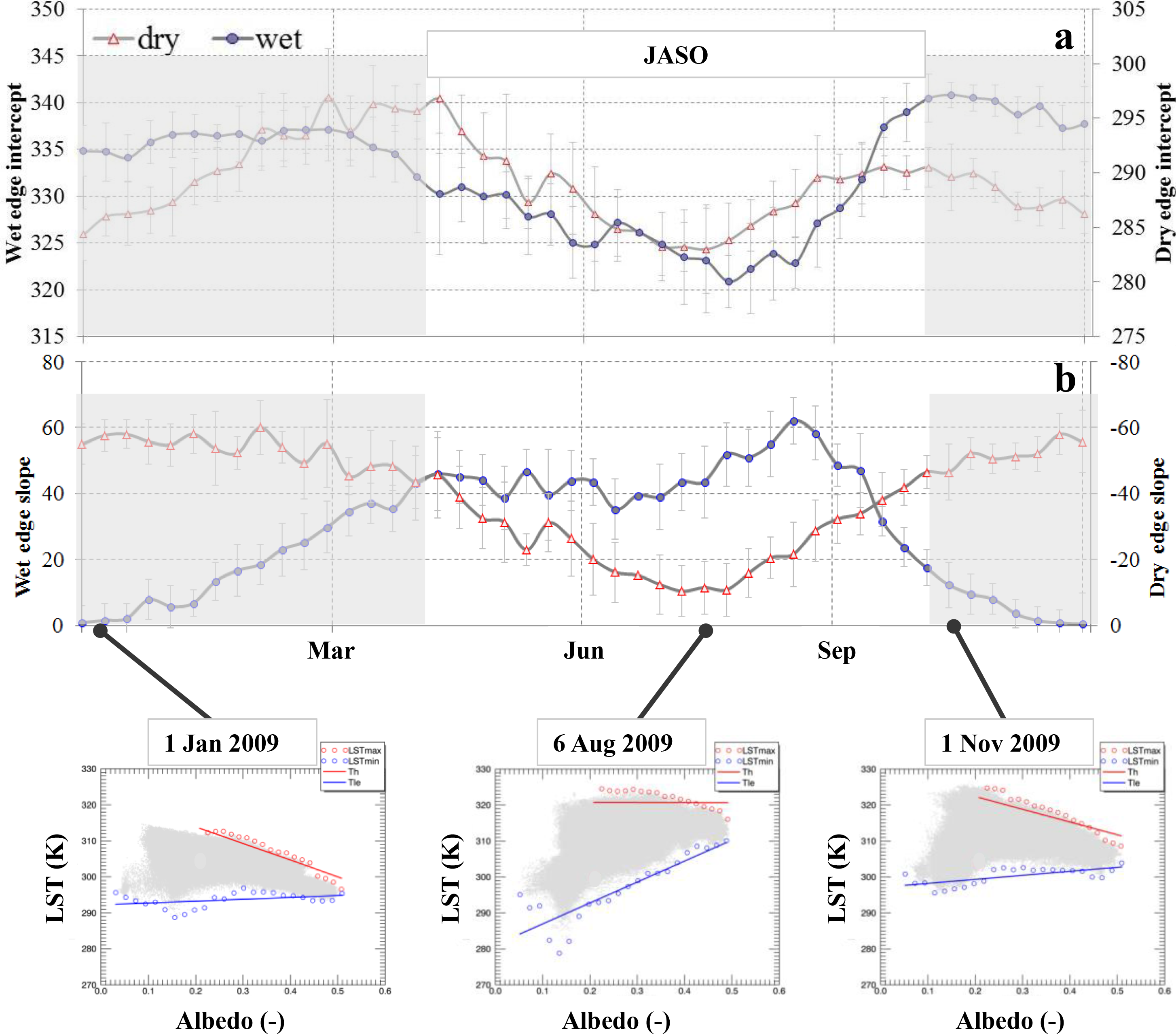
5.1. Dry and Wet Edge Statistics
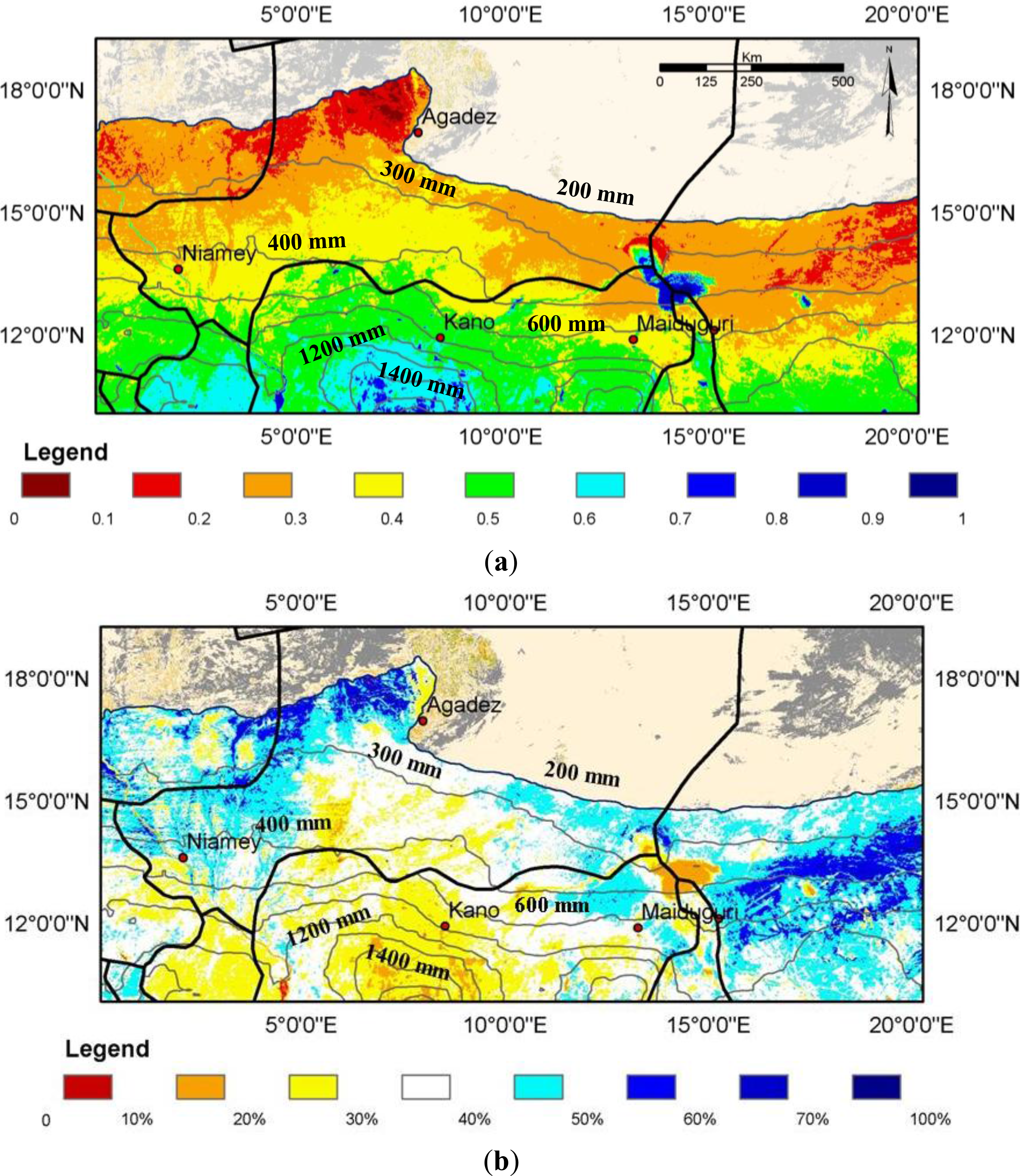
5.2. Evaluation of EF Spatial Patterns
5.3. Comparison of Seasonal EF Estimations with Eddy Covariance Data
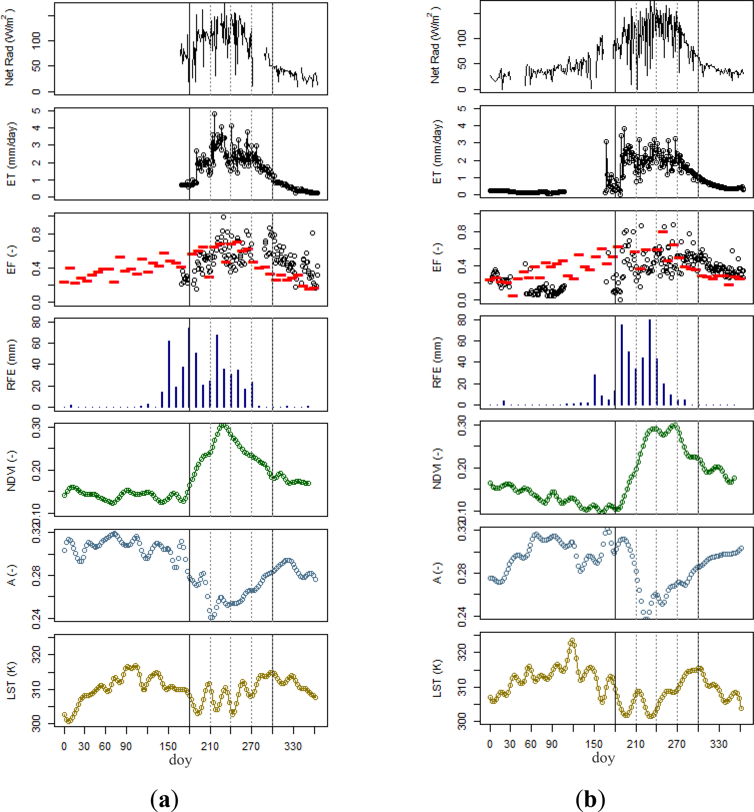
5.3.1. Temporal Dynamics of the Variables
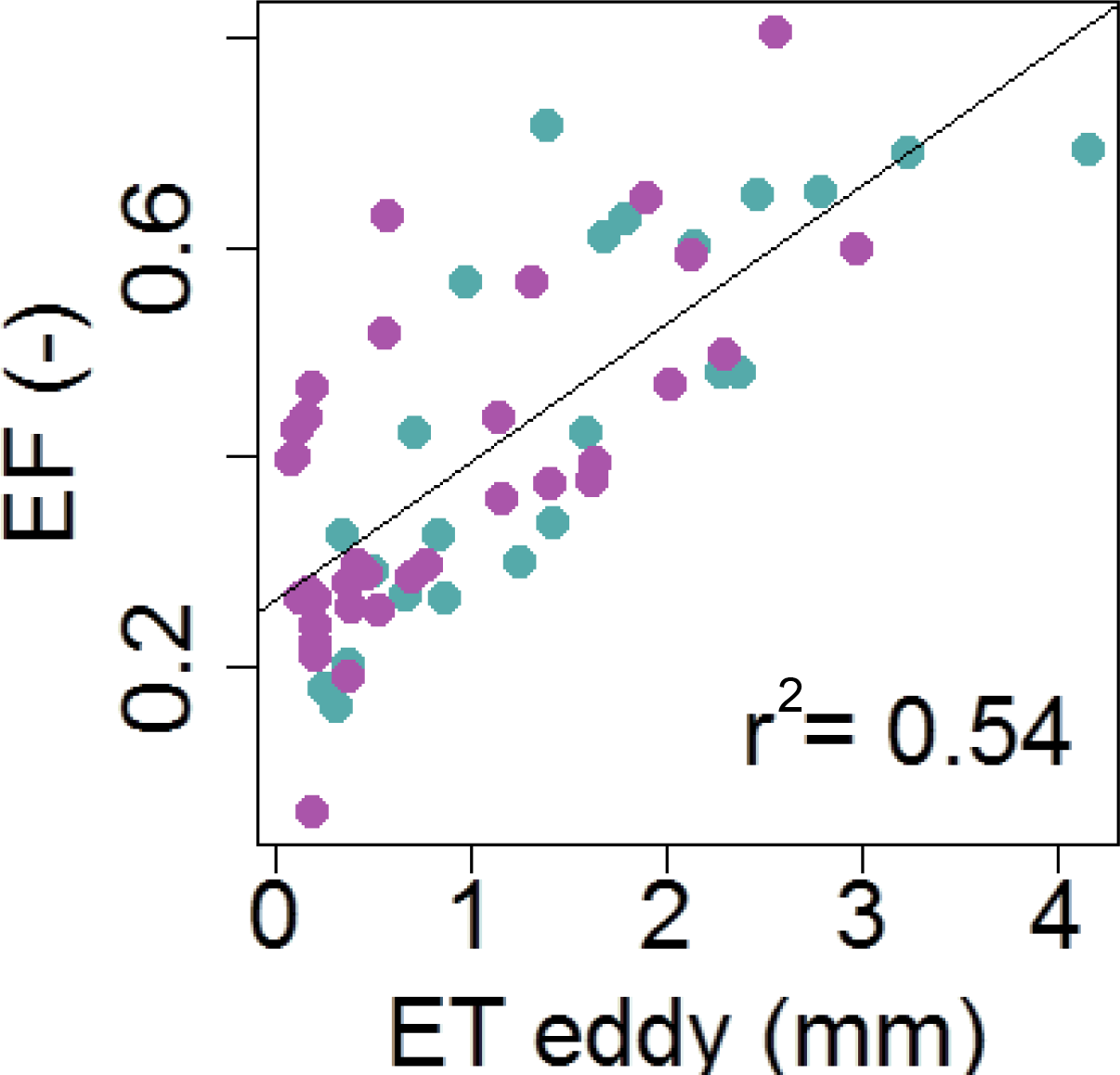
5.3.2. Correlation Analysis with ET
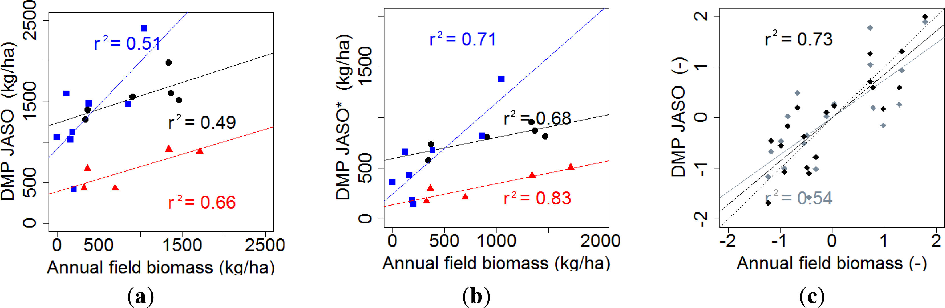
5.3.3. Biomass Estimation Improvements Using EF Correction
6. Conclusions
Acknowledgments
Author Contributions
Conflicts of Interest
References
- Anyamba, A.; Tucker, C. Analysis of Sahelian vegetation dynamics using NOAA-AVHRR NDVI data from 1981–2003. J. Arid Environ 2005, 63, 596–614. [Google Scholar]
- Zorom, M.; Barbier, B.; Mertz, O.; Servat, E. Diversification and adaptation strategies to climate variability: A farm typology for the Sahel. Agric. Syst 2013, 116, 7–15. [Google Scholar]
- Soler, C.M.T.; Maman, N.; Zhang, X.; Mason, S.C.; Hoogenboom, G. Determining optimum planting dates for pearl millet for two contrasting environments using a modelling approach. J. Agric. Sci 2008, 146, 445–459. [Google Scholar]
- Mortimore, M.J.; Adams, W.M. Farmer adaptation, change and “crisis” in the Sahel. Glob. Environ. Chang 2001, 11, 49–57. [Google Scholar]
- FAO. Available online: www.fao.org/emergencies/crisis/sahel/en (accessed on 14 April 2014).
- Mertz, O.; Mbow, C.; Maiga, A.; Diallo, D.; Reenberg, A.; Diouf, A.; Barbier, B.; Moussa, I.B.; Zorom, M.; Ouattara, I.; et al. Climate factors play a limited role for past adaptation strategies in West Africa. Ecol. Soc 2010, 15. Available on line: http://www.ecologyandsociety.org/vol15/iss4/art25/ (accessed on 14 April 2014). [Google Scholar]
- Wang, J.; Li, X.; Lu, L.; Fang, F. Estimating near future regional corn yields by integrating multi-source observations into a crop growth model. Eur. J. Agron 2013, 49, 126–140. [Google Scholar]
- Tucker, C.J.; Vanpraet, C.L.; Sharman, M.J.; van Ittersum, G. Satellite remote sensing of total herbaceous biomass production in the senegalese sahel: 1980–1984. Remote Sens. Environ 1985, 17, 233–249. [Google Scholar]
- Hein, L.; de Ridder, N.; Hiernaux, P.; Leemans, R.; de Wit, A.; Schaepman, M. Desertification in the Sahel: Towards better accounting for ecosystem dynamics in the interpretation of remote sensing images. J. Arid Environ 2011, 75, 1164–1172. [Google Scholar]
- Boschetti, M.; Nutini, F.; Brivio, P.A.; Bartholomé, E.; Stroppiana, D.; Hoscilo, A. Identification of environmental anomaly hot spots in West Africa from time series of NDVI and rainfall. ISPRS J. Photogramm. Remote Sens 2013, 78, 26–40. [Google Scholar]
- Olsson, L.; Eklundh, L.; Ardo, J. A recent greening of the Sahel—Trends, patterns and potential causes. J. Arid Environ 2005, 63, 556–566. [Google Scholar]
- Seaquist, J.; Hickler, T.; Eklundh, L. Disentangling the effects of climate and people on Sahel vegetation dynamics. Biogeosciences 2009, 6, 469–477. [Google Scholar]
- Herrmann, S.; Anyamba, A.; Tucker, C. Recent trends in vegetation dynamics in the African Sahel and their relationship to climate. Glob. Environ. Chang 2005, 15, 394–404. [Google Scholar]
- Huber, S.; Fensholt, R.; Rasmussen, K. Water availability as the driver of vegetation dynamics in the African Sahel from 1982 to 2007. Glob. Planet. Chang 2011, 76, 186–195. [Google Scholar]
- Fensholt, R.; Rasmussen, K. Analysis of trends in the Sahelian “rain-use efficiency” using GIMMS NDVI, RFE and GPCP rainfall data. Remote Sens. Environ 2011, 115, 438–451. [Google Scholar]
- Sandholt, I.; Rasmussen, K.; Andersen, J. A simple interpretation of the surface temperature/vegetation index space for assessment of surface moisture status. Remote Sens. Environ 2002, 79, 213–224. [Google Scholar]
- Bastiaanssen, W.G.M.; Menenti, M.; Feddes, R.A.; Holtslag, A.A.M. A remote sensing surface energy balance algorithm for land (SEBAL). 1. Formulation. J. Hydrol 1998, 212–213, 198–212. [Google Scholar]
- Verstraeten, W.W.; Veroustraete, F.; Feyen, J. Estimating evapotranspiration of European forests from NOAA-imagery at satellite overpass time: Towards an operational processing chain for integrated optical and thermal sensor data products. Remote Sens. Environ 2005, 96, 256–276. [Google Scholar]
- Allen, R.; Tasumi, M.; Trezza, R. Satellite-based energy balance for mapping evapotranspiration with internalized calibration (METRIC)—Model. J. Irrig. Drain. Eng 2007, 380–394. [Google Scholar]
- Irmak, A.; Ratcliffe, I.; Hubbard, K. Estimation of land surface evapotranspiration with a satellite remote sensing procedure. Gt. Plains Res 2011, 21, 73–88. [Google Scholar]
- Li, X.; Lu, L.; Yang, W.; Cheng, G. Estimation of evapotranspiration in an arid region by remote sensing—A case study in the middle reaches of the Heihe River Basin. Int. J. Appl. Earth Obs. Geoinf 2012, 17, 85–93. [Google Scholar]
- Sun, Z.; Gebremichael, M.; Ardö, J.; Nickless, A.; Caquet, B.; Merboldh, L.; Kutschi, W. Estimation of daily evapotranspiration over Africa using MODIS/Terra and SEVIRI/MSG data. Atmos. Res 2012, 112, 35–44. [Google Scholar]
- Hall, F.; Huemmrich, K. Satellite remote sensing of surface energy balance: Success, failures, and unresolved issues in FIFE. J. Geophys. Res 1992, 97, 19061–19089. [Google Scholar]
- Cragoa, R.; Brutsaert, W. Daytime evaporation and the self-preservation of the evaporative fraction and the Bowen ratio. J. Hydrol 1996, 178, 241–255. [Google Scholar]
- Crago, R.D. Conservation and variability of the evaporative fraction during the daytime. J. Hydrol 1996, 180, 173–194. [Google Scholar]
- Sobrino, J.A.; Gómez, M.; Jiménez-Muñoz, J.C.; Olioso, A. Application of a simple algorithm to estimate daily evapotranspiration from NOAA–AVHRR images for the Iberian Peninsula. Remote Sens. Environ 2007, 110, 139–148. [Google Scholar]
- Gomez, M.; Olioso, A.; Sobrino, J.; Jacob, F. Retrieval of evapotranspiration over the Alpilles/ReSeDA experimental site using airborne POLDER sensor and a thermal camera. Remote Sens. Environ 2005, 96, 399–408. [Google Scholar]
- Ciraolo, G.; Minacapilli, M.; Sciortino, M. Stima dell’evapotraspirazione effettiva mediante telerilevamento aereo iperspettrale. J. Agric. Eng 2007, 38, 49–60. [Google Scholar]
- Gentine, P.; Entekhabi, D.; Chehbouni, A.; Boulet, G.; Duchemin, B. Analysis of evaporative fraction diurnal behaviour. Agric. For. Meteorol 2007, 143, 13–29. [Google Scholar] [Green Version]
- Venturini, V.; Islam, S.; Rodriguez, L. Estimation of evaporative fraction and evapotranspiration from MODIS products using a complementary based model. Remote Sens. Environ 2008, 112, 132–141. [Google Scholar]
- Yang, D.; Chen, H.; Lei, H. Analysis of the diurnal pattern of evaporative fraction and its controlling factors over croplands in the Northern China. J. Integr. Agric 2013, 12, 1316–1329. [Google Scholar]
- Hoedjes, J.C.B.; Chehbouni, A.; Jacob, F.; Ezzahar, J.; Boulet, G. Deriving daily evapotranspiration from remotely sensed instantaneous evaporative fraction over olive orchard in semi-arid Morocco. J. Hydrol 2008, 354, 53–64. [Google Scholar]
- Bastiaanssen, W.G.M.; Ali, S. A new crop yield forecasting model based on satellite measurements applied across the Indus Basin, Pakistan. Agric. Ecosyst. Environ 2003, 94, 321–340. [Google Scholar]
- Bastiaanssen, W.G.M.; Pelgrum, H.; Droogers, P.; de Bruin, H.A.R.; Menenti, M. Area-average estimates of evaporation, wetness indicators and top soil moisture during two golden days in EFEDA. Agric. For. Meteorol 1997, 87, 119–137. [Google Scholar]
- Kustas, W.; Schmugge, T.; Humes, K.; Jackson, T.; Parry, R.; Weltz, M.; Moran, M. Relationships between evaporative fraction and remotely sensed vegetation index and microwave brightness temperature for semiarid rangelands. J. Appl. Metereol 1993, 32, 1781–1790. [Google Scholar]
- Kurc, S.A.; Small, E.E. Dynamics of evapotranspiration in semiarid grassland and shrubland ecosystems during the summer monsoon season, central New Mexico. Water Resour. Res 2004, 40. [Google Scholar] [CrossRef]
- Guyot, A.; Cohard, J.-M.; Anquetin, S.; Galle, S. Long-term observations of turbulent fluxes over heterogeneous vegetation using scintillometry and additional observations: A contribution to AMMA under Sudano-Sahelian climate. Agric. For. Meteorol 2012, 154–155, 84–98. [Google Scholar]
- Higuchi, A.; Kondoh, A.; Kishi, S. Relationship among the surface albedo, spectral reflectance of canopy, and evaporative fraction at grassland and paddy field. Adv. Space Res 2000, 26, 1043–1046. [Google Scholar]
- Yuan, W.; Liu, S.; Zhou, G.; Zhou, G.; Tieszen, L.L.; Baldocchi, D.; Bernhofer, C.; Gholz, H.; Goldstein, A.H.; Goulden, M.L.; et al. Deriving a light use efficiency model from eddy covariance flux data for predicting daily gross primary production across biomes. Agric. For. Meteorol 2007, 143, 189–207. [Google Scholar]
- Kanniah, K.D.; Beringer, J.; Hutley, L.B.; Tapper, N.J.; Zhu, X. Evaluation of Collections 4 and 5 of the MODIS Gross Primary Productivity product and algorithm improvement at a tropical savanna site in northern Australia. Remote Sens. Environ 2009, 113, 1808–1822. [Google Scholar]
- Sjöström, M.; Ardö, J.; Arneth, A.; Boulain, N.; Cappelaere, B.; Eklundh, L.; de Grandcourt, A.; Kutsch, W.L.; Merbold, L.; Nouvellon, Y. Exploring the potential of MODIS EVI for modeling gross primary production across African ecosystems. Remote Sens. Environ 2011, 115, 1081–1089. [Google Scholar]
- Jiang, L.; Islam, S. Estimation of surface evaporation map over southern Great Plains using remote sensing data. Water Resour. Res 2001, 37, 329–340. [Google Scholar]
- Roerink, G.; Su, Z.; Menenti, M. S-SEBI: A simple remote sensing algorithm to estimate the surface energy balance. Phys. Chem. Earth Part B 2000, 25, 147–157. [Google Scholar]
- Galleguillos, M.; Jacob, F.; Prévot, L.; French, A.; Lagacherie, P. Comparison of two temperature differencing methods to estimate daily evapotranspiration over a Mediterranean vineyard watershed from ASTER data. Remote Sens. Environ 2011, 115, 1326–1340. [Google Scholar]
- Olivera-Guerra, L.; Mattar, C.; Galleguillos, M. Estimation of real evapotranspiration and its variation in Mediterranean landscapes of central-southern Chile. Int. J. Appl. Earth Obs. Geoinf 2014, 28, 160–169. [Google Scholar]
- Santos, C.A.C.; Bezerra, B.G.; Silva, B.B.; Rao, T.V.R. Assessment of daily actual evapotranspiration with SEBAL and S-SEBI algorithms in cotton crop. Rev. Bras. Meteorol 2010, 25, 383–398. [Google Scholar]
- Wang, K.; Dickinson, R. A review of global terrestrial evapotranspiration: Observation, modeling, climatology, and climatic variability. Rev. Geophys 2012, 50, 1–54. [Google Scholar]
- Ramankutty, N. Croplands in West Africa: A geographically explicit dataset for use in models. Earth Interact 2004, 8, 1–22. [Google Scholar]
- CRED Emergency Events Database. Available online: http://www.emdat.be/result-country-profile (accessed on 14 April 2014).
- Brink, A.B.; Eva, H.D. Monitoring 25 years of land cover change dynamics in Africa: A sample based remote sensing approach. Appl. Geogr 2009, 29, 501–512. [Google Scholar]
- Arino, O.; Gross, D.; Ranera, F.; Leroy, M.; Bicheron, P.; Brockman, C.; Defourny, P.; Vancutsem, C.; Achard, F.; Durieux, L.; et al. GlobCover: ESA Service for Global Land Cover from MERIS. Proceedings of the IEEE International Geoscience and Remote Sensing Symposium, IGARSS 2007, Barcelona, Spain, 23–28 July 2007; pp. 2412–2415.
- USGS MODIS Data Products Table. Available online: https://lpdaac.usgs.gov/products/modis_products_table (accessed on 14 April 2014).
- Smets, B.; Eerens, H.; Jacobs, T.; Royer, A. BioPar Dry Matter Productivity (DMP) Product User Manual. Available online: http://web.vgt.vito.be/documents/BioPar/g2-BP-RP-BP053-ProductUserManual-DMPV0-I1.00.pdf (accessed on 14 April 2014).
- NOAA CPC The NOAA Climate Prediction Center African Rainfall Estimation Algorithm Version 2.0. Available online: http://www.cpc.ncep.noaa.gov/products/fews/RFE2.0_tech.pdf (accessed on 14 April 2014).
- VITO Low & Medium Resolution EO-Products—Free Data. Available online: www.vito-eodata.be(accessed on 14 April 2014).
- Justice, C.; Hiernaux, P. Monitoring the grasslands of the Sahel using NOAA AVHRR data: Niger 1983. Int. J. Remote Sens 1986, 7, 37–41. [Google Scholar]
- Bonifacio, R.; Dugdale, G.; Milford, J. Sahelian rangeland production in relation to rainfall estimates from Meteosat. Int. J. Remote Sens 1993, 14, 2695–2711. [Google Scholar]
- Mutanga, O.; Skidmore, A. Merging double sampling with remote sensing for a rapid estimation of fuelwood. Geocarto Int 2004, 19. [Google Scholar] [CrossRef]
- Ham, F.; Fillol, E. Pastoral Surveillance System and Feed Inventory in the Sahel. In Conducting National Feed Assessments; FAO: Rome, Italy, 2010; Volume 1998, pp. 83–114. [Google Scholar]
- Oak Ridge National Laboratory Distributed Active Archive Center FLUXNET Web Page. Available online: http://fluxnet.ornl.gov (accessed on 14 April 2014).
- Mauder, M.; Liebethal, C.; Göckede, M.; Leps, J.-P.; Beyrich, F.; Foken, T. Processing and quality control of flux data during LITFASS-2003. Bound. Layer Meteorol 2006, 121, 67–88. [Google Scholar]
- Ramier, D.; Boulain, N.; Cappelaere, B.; Timouk, F.; Rabanit, M.; Lloyd, C.R.; Boubkraoui, S.; Métayer, F.; Descroix, L.; Wawrzyniak, V. Towards an understanding of coupled physical and biological processes in the cultivated Sahel—1. Energy and water. J. Hydrol 2009, 375, 204–216. [Google Scholar]
- Sturges, H. The choice of a class interval. J. Am. Stat. Assoc 1926, 21, 65–66. [Google Scholar]
- De Castro Teixeira, A.H.; Bastiaanssen, W.G.M.; Ahmad, M.D.; Moura, M.S.B.; Bos, M.G. Analysis of energy fluxes and vegetation-atmosphere parameters in irrigated and natural ecosystems of semi-arid Brazil. J. Hydrol 2008, 362, 110–127. [Google Scholar]
- Fensholt, R.; Sandholt, I.; Rasmussen, M.S.; Stisen, S.; Diouf, A. Evaluation of satellite based primary production modelling in the semi-arid Sahel. Remote Sens. Environ 2006, 105, 173–188. [Google Scholar]
- Seaquist, J. A remote sensing-based primary production model for grassland biomes. Ecol. Modell 2003, 169, 131–155. [Google Scholar]
- Meroni, M.; Fasbender, D.; Kayitakire, F.; Pini, G.; Rembold, F.; Urbano, F.; Verstraete, M.M. Early detection of biomass production deficit hot-spots in semi-arid environment using FAPAR time series and a probabilistic approach. Remote Sens. Environ 2014, 142, 57–68. [Google Scholar]
- Loague, K.M.; Green, R.E. Statistical and graphical methods for evaluating solute transport models: Overview and application. J. Contam. Hydrol 1991, 7, 51–73. [Google Scholar]
- Akaike, H. A new look at the statistical model identification. IEEE Trans. Autom. Control 1974, 19, 716–723. [Google Scholar]
- Bagayoko, F.; Yonkeu, S.; Elbers, J.; van de Giesen, N. Energy partitioning over the West African savanna: Multi-year evaporation and surface conductance measurements in Eastern Burkina Faso. J. Hydrol 2007, 334, 545–559. [Google Scholar]
- Son, N.T.; Chen, C.F.; Chen, C.R.; Chang, L.Y.; Minh, V.Q. Monitoring agricultural drought in the Lower Mekong Basin using MODIS NDVI and land surface temperature data. Int. J. Appl. Earth Obs. Geoinf 2012, 18, 417–427. [Google Scholar]
- Coakley, J. Reflectance and Albedo, Surface. Available online: http://curry.eas.gatech.edu/Courses/6140/ency/Chapter9/Ency_Atmos/Reflectance_Albedo_Surface.pdf (accessed on 14 April 2014).
- ECOWAS-SWAC. The Ecologically Vulnerable Zone of Sahelian Countries. In Atlas on Regional Integration in West Africa; ECOWAS—SWAC/OECD: Abuja, Nigeria, 2006; pp. 2–12. [Google Scholar]
- Leblanc, M.; Lemoalle, J.; Bader, J.; Tweed, S. Thermal remote sensing of water under flooded vegetation: New observations of inundation patterns for the Small’Lake Chad. J. Hydrol 2011, 404, 87–98. [Google Scholar]
- Nutini, F.; Boschetti, M.; Brivio, P.; Bocchi, S.; Antoninetti, M. Land-use and land-cover change detection in a semi-arid area of Niger using multi-temporal analysis of Landsat images. Int. J. Remote Sens 2013, 34, 37–41. [Google Scholar]
- Campbell, B.D.; Stafford Smith, D.M. A synthesis of recent global change research on pasture and rangeland production: Reduced uncertainties and their management implications. Agric. Ecosyst. Environ 2000, 82, 39–55. [Google Scholar]
- Barbosa, H.A.; Huete, A.R.; Baethgen, W.E. A 20-year study of NDVI variability over the Northeast Region of Brazil. J. Arid Environ 2006, 67, 288–307. [Google Scholar]


| Site | #Data | Period | AVG (kg/ha) | Max (kg/ha) | Min (kg/ha) | Stand Deviation (kg/ha) |
|---|---|---|---|---|---|---|
| Site 1 | 6 | 2003; 2005–2009 | 963 | 1,463 | 342 | 508 |
| Site 2 | 8 | 2000; 2002–2009 | 371 | 1,047 | 0 | 378 |
| Site 3 | 5 | 2001; 2005; 2007–2009 | 888 | 1712 | 326 | 614 |
© 2014 by the authors; licensee MDPI, Basel, Switzerland This article is an open access article distributed under the terms and conditions of the Creative Commons Attribution license (http://creativecommons.org/licenses/by/3.0/).
Share and Cite
Nutini, F.; Boschetti, M.; Candiani, G.; Bocchi, S.; Brivio, P.A. Evaporative Fraction as an Indicator of Moisture Condition and Water Stress Status in Semi-Arid Rangeland Ecosystems. Remote Sens. 2014, 6, 6300-6323. https://doi.org/10.3390/rs6076300
Nutini F, Boschetti M, Candiani G, Bocchi S, Brivio PA. Evaporative Fraction as an Indicator of Moisture Condition and Water Stress Status in Semi-Arid Rangeland Ecosystems. Remote Sensing. 2014; 6(7):6300-6323. https://doi.org/10.3390/rs6076300
Chicago/Turabian StyleNutini, Francesco, Mirco Boschetti, Gabriele Candiani, Stefano Bocchi, and Pietro Alessandro Brivio. 2014. "Evaporative Fraction as an Indicator of Moisture Condition and Water Stress Status in Semi-Arid Rangeland Ecosystems" Remote Sensing 6, no. 7: 6300-6323. https://doi.org/10.3390/rs6076300