Remote Sensing Assessment of Forest Disturbance across Complex Mountainous Terrain: The Pattern and Severity of Impacts of Tropical Cyclone Yasi on Australian Rainforests

 ,
, 
Abstract
:1. Introduction
2. Study Area and Dataset
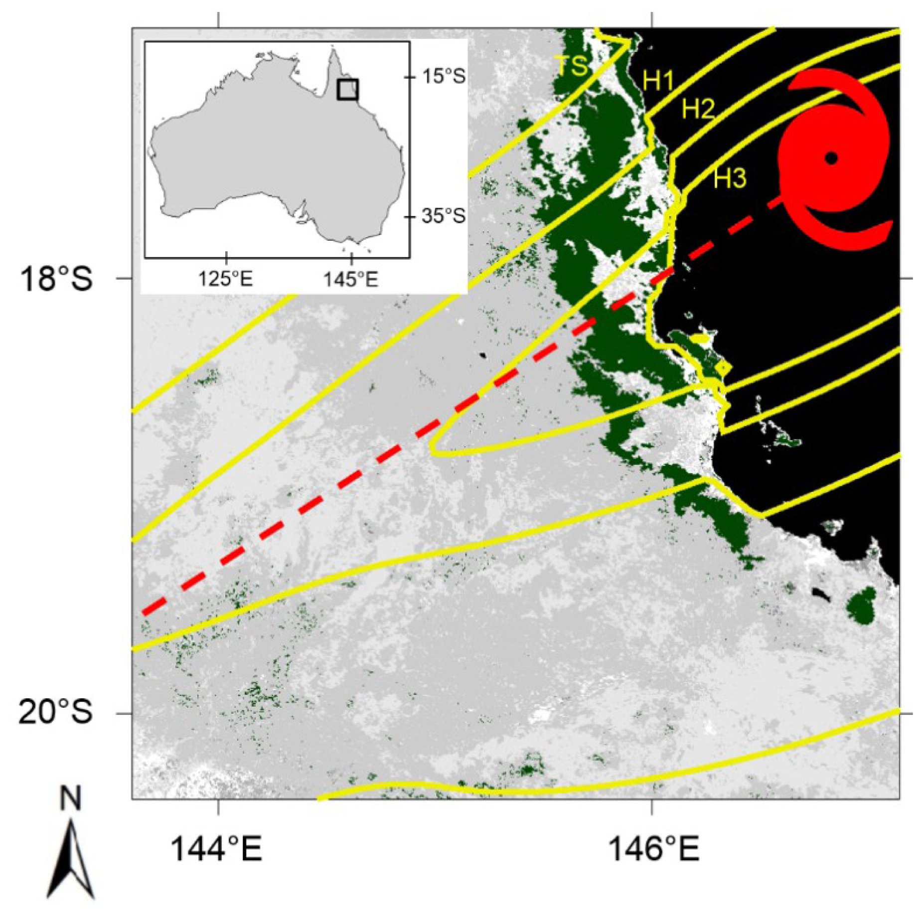
2.1. Study Area
2.2. Yasi’s Surface Wind Data
2.3. Multispectral Data
2.4. Topography Data and Carbon Map
3. Method
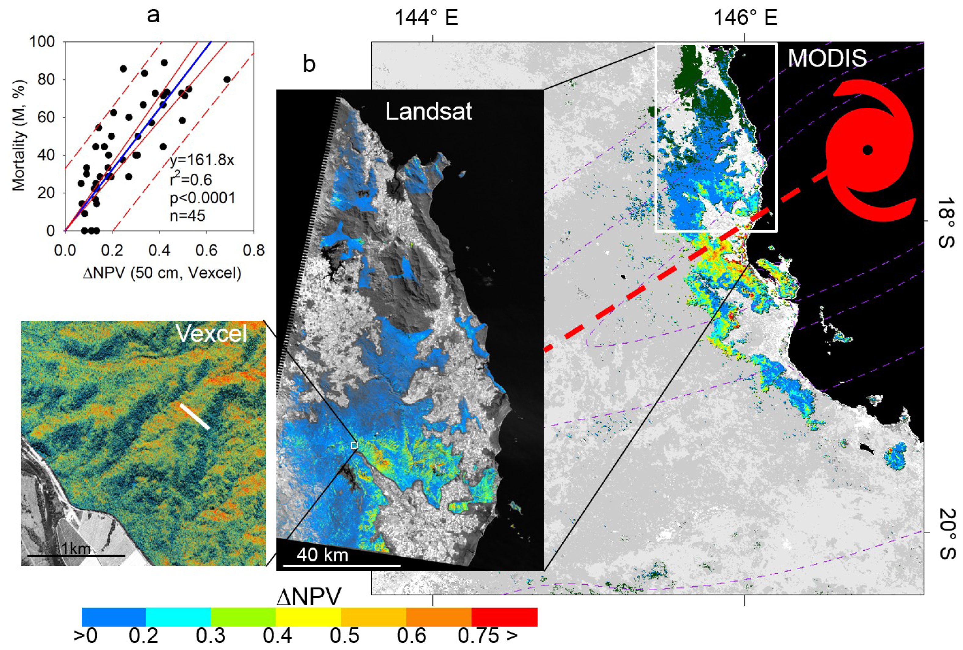
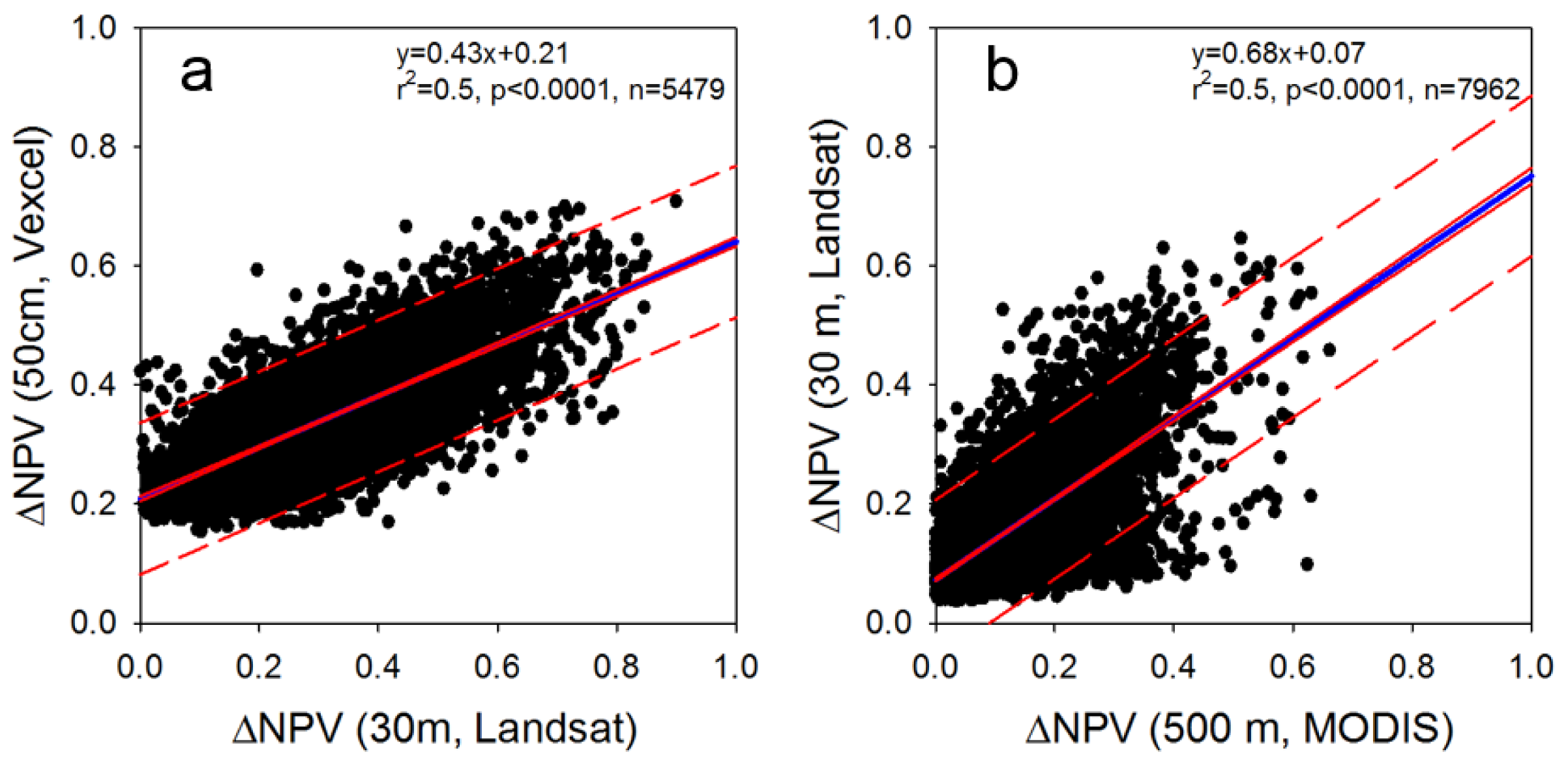
4. Results
5. Discussion
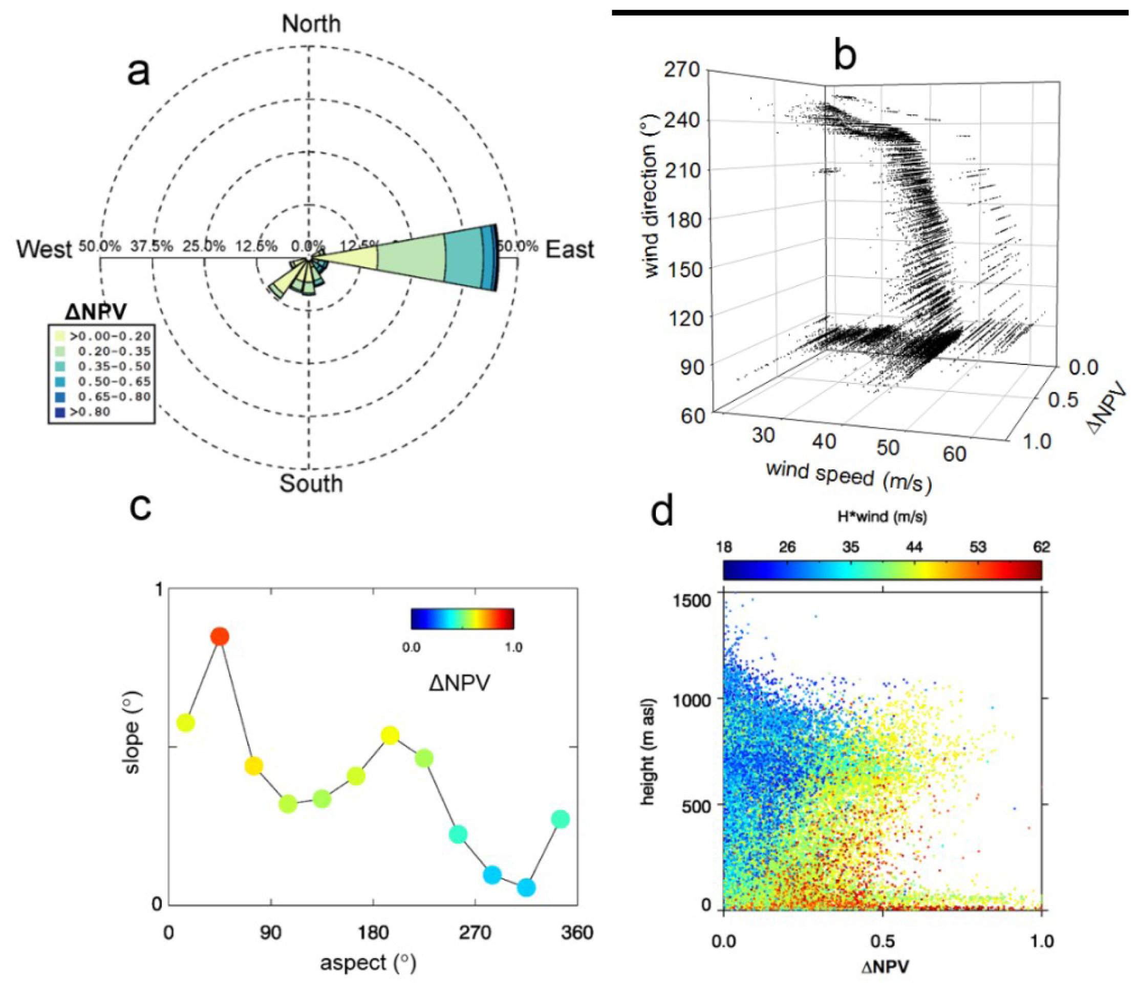
5.1. Patterns of Forest Disturbance Associated with Topography
5.2. Disturbance Severity and Forests Type
5.3. Assessment of tree Mortality and Committed Carbon
5.4. Uncertainties, Errors, and Accuracy Issues
6. Conclusions
Supplementary Information
remotesensing-06-05633-s001.pdfAcknowledgments
Conflicts of Interest
- Author ContributionsAll authors contributed extensively to the work. Robinson Negrón-Juárez, Jeffrey Chambers and George Hurtt designed and performed the experiment. Bachir Annane, Stephen Cocke, and Mark Powell produced the H*wind data and contributed significantly to the analysis, interpretation and discussion of results. Stephen Goosem, Michael Stott, Daniel J. Metcalfe and Sassan S. Saatchi provided the ecological data and contributed significantly to the analysis, interpretation and discussion of results. Robinson Negrón-Juárez wrote the manuscript. Stephen Goosem edited the manuscript.
References
- World Meteorological Organization. Available online: http://www.wmo.int,tropicalcyclones (accessed on 5 December 2013).
- Foster, D.; Boose, E. Patterns of forest damage resulting from catastrophic wind in central New England, U.S.A. J. Ecol 1992, 80, 79–98. [Google Scholar]
- Metcalfe, D.; Bradford, M.; Ford, A. Cyclone damage to tropical rain forests: Species- and community-level impacts. Austral Ecol 2008, 33, 432–441. [Google Scholar]
- Lugo, A. Visible and invisible effects of hurricanes on forest ecosystems: An international review. Austral Ecol 2008, 33, 369–398. [Google Scholar]
- Everham, E.; Brokaw, N.V. Forest damage and recovery from catastrophic wind. Bot. Rev 1996, 62, 113–185. [Google Scholar]
- Van Bloem, S.; Murphy, P.; Lugo, A.; Ostertag, R.; Costa, M.; Bernard, I.; Colon, S.; Mora, M. The influence of hurricane winds on Caribbean dry forest structure and nutrient pools. Biotropica 2005, 37, 571–583. [Google Scholar]
- Turton, S. Landscape-scale impacts of Cyclone Larry on the forest of northern Australia, including comparisons with previous cyclones impacting the region between 1858 and 2006. Austral Ecol 2008, 33, 409–416. [Google Scholar]
- Chambers, J.; Fisher, J.; Zeng, H.; Chapman, E.; Baker, D.; Hurtt, G. Hurricane Katrina’s carbon footprint on U.S. Gulf Coast forest. Science 2007, 318. [Google Scholar] [CrossRef]
- Negrón-Juárez, R.; Chambers, J.; Zeng, H.; Baker, D. Hurricane driven changes in land cover create biogeophysical climate feedbacks. Geophys. Res. Lett 2008, 35. [Google Scholar] [CrossRef]
- Boose, E.; Serrano, M.; Foster, D. Landscape and regional impacts of hurricanes in Puerto Rico. Ecol. Monogr 2004, 74, 335–352. [Google Scholar]
- Xi, W.; Peet, R.; Decoster, J.; Urban, D. Tree damage risk factors associated with large, infrequent wind disturbances of Carolina forests. Forestry 2008, 81, 317–334. [Google Scholar]
- Masek, J.; Huang, C.; Wolfe, R.; Cohen, W.; Hall, F.; Kutler, J.; Nelson, P. North American forest disturbance mapped from a decadal Landsat record. Remote Sens. Environ 2008, 112, 2914–2926. [Google Scholar]
- Frolking, S.; Palace, M.; Clark, D.; Chambers, J.; Shugart, H.; Hurtt, G. Forest disturbance and recovery: A general review in the context of spaceborne remote sensing of impacts on aboveground biomass and canopy structure. J. Geophys. Res 2009, 114, 1–27. [Google Scholar]
- Huang, C.; Goward, S.N.; Masek, J.G.; Thomas, N.; Zhu, Z.; Vogelmann, J.E. An automated approach for reconstructing recent forest disturbance history using dense Landsat time series stacks. Remote Sens. Environ 2010, 114, 183–198. [Google Scholar]
- Kennedy, R.E.; Yang, Z.; Cohen, W.B. Detecting trends in forest disturbance and recovery using yearly Landsat time series: 1. LandTrendr—Temporal segmentation algorithms. Remote Sens. Environ 2010, 114, 2897–2910. [Google Scholar]
- Zhu, Z.; Woodcock, C.E.; Olofsson, P. Continuous monitoring of forest disturbance using all available Landsat imagery. Remote Sens. Environ 2012, 122, 75–91. [Google Scholar]
- Negrón-Juárez, R.; Baker, D.; Zeng, H.; Henkel, T.; Chambers, J. Assessing hurricane-induced tree mortality in U.S. Gulf Coast forest ecosystems. J. Geophys. Res. Biogeo 2010, 115. [Google Scholar] [CrossRef]
- Negrón-Juárez, R.; Baker, D.; Chambers, J.; Hurtt, G.; Goosem, S. Multi-scale sensitivity of Landsat and MODIS to forest disturbance associated with tropical cyclones. Remote Sens. Environ 2014, 140, 679–689. [Google Scholar]
- Boose, E.; Foster, D.; Fluet, M. Hurricane impacts to tropical and temperate forest landscapes. Ecol. Monogr 1994, 64, 369–400. [Google Scholar]
- Intergovernmental Panel on Climate Change, Climate Change 2007: The Physical Science Basis. In Contribution of Working Group I to the Fourth Assessment Report of the Intergovernmental Panel on Climate Change; Solomon, S.; Qin, D.; Manning, M.; Chen, Z.; Marquis, M.; Averyt, K.B.; Tignor, M.; Miller, H.L. (Eds.) Cambridge University Press: New York, NY, USA, 2007.
- Saatchi, S.; Harrys, N.; Brown, S.; Lefsky, M.; Mitchard, E.; Salas, W.; Zutta, B.; Buemann, W.; Lewis, S.; Hagen, S.; et al. Benchmark map of forest carbon stock in tropical regions across three continents. Proc. Natl. Acad. Sci. USA 2011, 108, 9899–9904. [Google Scholar]
- The Saffir-Simpson Hurricane Wind Scale. Available online: http://www.nhc.noaa.gov/pdf/sshws.pdf (accessed on 5 December 2013).
- Severe Tropical Cyclone Yasi—Bureau of Meteorology. Available online: http://www.bom.gov.au/cyclone/history/yasi.shtml (accessed on 5 December 2013).
- Webb, L. Cyclones as an ecological factor in tropical lowland rainforest, North Queensland. Aust. J. Bot 1958, 6, 220–228. [Google Scholar]
- Wet Tropics Management Authority—Wet Tropics World Heritage Area. Available online: http://www.wettropics.gov.au (accessed on 5 December 2013).
- Metcalfe, D.; Ford, A. Floristic Biodiversity in the Wet Tropics. In Chapter 7 in Living in a Dynamic Tropical Forest Landscape; Stork, N., Turton, S., Eds.; Blackwell: Oxford, UK, 2008; pp. 123–132. [Google Scholar]
- Metcalfe, D.; Ford, A. A re-evaluation of Queensland’s Wet Tropics based on primitive plants. Pac. Conserv. Biol 2009, 15, 80–86. [Google Scholar]
- Goosem, S.; Morgan, G.; Kemp, J. Wet Tropics. In The Conservation Status of Queensland’s Bioregional Ecosystems; Sattler, P.S., Williams, R.D., Eds.; Environmental Protection Agency: Brisbane, Australia, 1999; pp. 7/1–7/73. [Google Scholar]
- Powell, M.D.; Houston, S.; Amat, L.; Morisseau-Leroy, N. The HRD real-time hurricane wind analysis system. J. Wind Eng. Ind. Aerodyn 1998, 77–78, 53–64. [Google Scholar]
- Powell, M.D.; Murillo, S.; Dodge, P.; Uhlhorn, E.; Gamache, J.; Cardone, V.; Cox, A.; Otero, S.; Carrasco, N.; Annane, B.; Fleur, R. Reconstruction of Hurricane Katrina’s wind fields for storm surge and wave hindcasting. Ocean Eng 2010, 37, 26–36. [Google Scholar]
- Yasi H*Wind Data. Available online: ftp://ftp.aoml.noaa.gov/hrd/pub/annane/Yasi (accessed on 5 December 2013).
- AEROmetrex. Available online: http://aerometrex.com.au (accessed on 5 December 2013).
- Dimap Australia. Available online: http://www.dimap.com.au (accessed on 5 December 2013).
- U.S. Geological Survey. Available online: http://calval.cr.usgs.gov (accessed on 5 December 2013).
- Vermote, E.; Kotchenva, S. Atmospheric correction for the monitoring of land surfaces. J. Geophys. Res 2008, 113. [Google Scholar] [CrossRef]
- Souza, C.; Roberts, D.; Cochrane, M. Combining spectral and spatial information to map canopy damage from selective logging and forest fires. Remote Sens. Environ 2005, 98, 329–343. [Google Scholar]
- NASA Land Data Products and Services-U.S. Geological Survey. Available online: https://lpdaac.usgs.gov (accessed on 5 December 2013).
- Adams, J.; Sabol, D.; Kapos, V.; Almeida Filho, R.; Roberts, D.; Smith, M.; Gillespie, A. Classification of multispectral images based on fractions of endmembers: Application to land-cover change in the Brazilian Amazon. Remote Sens. Environ 1995, 53, 137–154. [Google Scholar]
- Adams, J.B.; Gillespie, A.R. Remote Sensing of Landscapes with Spectral Images. In A Physical Modeling Approach; Cambridge University Press: Cambridge, UK, 2006. [Google Scholar]
- Boardman, J.; Kruse, F.; Green, R. Mapping Target Signatures via Partial Unmixing of AVIRIS Data. Proceedings of Fifth Annual JPL Airborne Earth Science Workshop, Pasadena, CA, USA, 23–26 January 1995; pp. 23–26.
- Chambers, J.Q.; Higuchi, C.; Schimel, J.; Fererira, L.; Melack, J. Decomposition and carbon cycling of dead trees in tropical forests of the central Amazon. Oecologia 2000, 122, 380–388. [Google Scholar]
- Eisenhauer, J. Regression through the Origin. Teach. Stat 2003, 25, 76–80. [Google Scholar]
- Houze, R. Clouds in tropical cyclones. Mon. Weather Rev 2010, 138, 293–344. [Google Scholar]
- Commonwealth of Australia, National Inventory Report-NIR 2010. Available online: http://climatechange.gov.au/sites/climatechange/files/documents/03_2013/national-inventory-report-2010-2.pdf (accessed on 29 January 2014).
- Brokaw, N.; Walker, L. Summary of the effects of Caribbean hurricanes on vegetation. Biotropica 1991, 23, 442–447. [Google Scholar]
- Ramsay, H.; Leslie, L. The effects of complex terrain on severe landfalling tropical Cyclone Larry (2006) over Northeast Australia. Mon. Weather Rev 2008, 136, 4334–4354. [Google Scholar]
- Asner, G.P. Cloud cover in Landsat observations of the Brazilian Amazon. Int. J. Remote Sens 2001, 22, 3855–3862. [Google Scholar]
- Knapp, K.; Kruk, M.; Levinson, D.; Diamond, H.; Neumann, C. The International Best Track Archive for Climate Stewardship (IBTrACS): Unifying tropical cyclone best track data. B. Am. Meteorol. Soc 2010, 91, 363–376. [Google Scholar]
- Gao, F.; Masek, J.; Schwaller, M.; Hall, F. On the blending of the Landsat and MODIS surface reflectance: Predicting daily Landsat surface reflectance. IEEE Trans. Geosci. Remote Sens 2006, 44, 2207–2218. [Google Scholar]
- Justice, C.O.; Townshend, J.R.G.; Vermote, E.F.; Masuoka, E.; Wolfe, R.E.; Saleous, N.; Roy, D.P.; Morisette, J.T. An overview of MODIS Land data processing and product status. Remote Sens. Environ 2002, 83, 3–15. [Google Scholar]
- Roy, D.P.; Ju, J.; Lewis, P.; Schaaf, C.; Gao, F.; Hansen, M.; Lindquist, E. Multi-temporal MODIS–Landsat data fusion for relative radiometric normalization, gap filling, and prediction of Landsat data. Remote Sens. Environ 2008, 112, 3112–3130. [Google Scholar]
- Hilker, T.; Wulder, M.A.; Coops, N.C.; Seitz, N.; White, J.C.; Gao, F.; Masek, J.G.; Stenhouse, G. Generation of dense time series synthetic Landsat data through data blending with MODIS using a spatial and temporal adaptive reflectance fusion model. Remote Sens. Environ 2009, 113, 1988–1999. [Google Scholar]
- Hubert, S.; Schwarzer, S.; Jaquet, J.M. Spatial degradation of classified satellite images. Open Remote Sens. J 2012, 5, 64–72. [Google Scholar]
- Arun, P.V.; Katiyar, S.K. Intelligent adaptive resampling technique for the processing of remotely sensed imagery. Ann. GIS 2014, 20, 53–60. [Google Scholar]
- Gupta, R.; Prassad, T.; Rao, P.; Manikavelu, B. Problems in upscaling of high resolution remote sensing data to coarse spatial resolution over land surface. Adv. Space Res 2000, 27, 1111–1121. [Google Scholar]
- Fisher, J.; Mustard, J. Cross-scalar satellite phenology from ground, Landsat and MODIS data. Remote Sens. Environ 2007, 109, 261–273. [Google Scholar]
- Roman, M.; Gateve, C.; Shuai, Y.; Wang, Z.; Gao, F.; Masek, J.; He, T.; Liang, S.; Schaaf, C. Use of in situ and airborne multiangle data to assess MODIS- and Landsat-based estimates of directional reflectance and albedo. IEEE Trans. Geosci. Remote Sens 2013, 51, 1393–1404. [Google Scholar]
- Turton, S. Securing landscape resilience to tropical cyclones in Australia’s wet tropics under a changing climate: lessons from cyclones Larry (and Yasi). Geogr. Res 2012, 50, 15–30. [Google Scholar]
- Aster GEM-NASA. Available online: http://asterweb.jpl.nasa.gov/gdem.asp (accessed on 5 December 2013).
- Roberts, D.; Gardner, M.; Church, R.; Ustin, S.; Scheer, G.; Green, R. Mapping chaparral in the Santa Monica Mountains using multiple endmember spectral mixture models. Remote Sens. Environ 1998, 65, 267–279. [Google Scholar]


© 2014 by the authors; licensee MDPI, Basel, Switzerland This article is an open access article distributed under the terms and conditions of the Creative Commons Attribution license (http://creativecommons.org/licenses/by/3.0/).
Share and Cite
Negrón-Juárez, R.I.; Chambers, J.Q.; Hurtt, G.C.; Annane, B.; Cocke, S.; Powell, M.; Stott, M.; Goosem, S.; Metcalfe, D.J.; Saatchi, S.S. Remote Sensing Assessment of Forest Disturbance across Complex Mountainous Terrain: The Pattern and Severity of Impacts of Tropical Cyclone Yasi on Australian Rainforests. Remote Sens. 2014, 6, 5633-5649. https://doi.org/10.3390/rs6065633
Negrón-Juárez RI, Chambers JQ, Hurtt GC, Annane B, Cocke S, Powell M, Stott M, Goosem S, Metcalfe DJ, Saatchi SS. Remote Sensing Assessment of Forest Disturbance across Complex Mountainous Terrain: The Pattern and Severity of Impacts of Tropical Cyclone Yasi on Australian Rainforests. Remote Sensing. 2014; 6(6):5633-5649. https://doi.org/10.3390/rs6065633
Chicago/Turabian StyleNegrón-Juárez, Robinson I., Jeffrey Q. Chambers, George C. Hurtt, Bachir Annane, Stephen Cocke, Mark Powell, Michael Stott, Stephen Goosem, Daniel J. Metcalfe, and Sassan S. Saatchi. 2014. "Remote Sensing Assessment of Forest Disturbance across Complex Mountainous Terrain: The Pattern and Severity of Impacts of Tropical Cyclone Yasi on Australian Rainforests" Remote Sensing 6, no. 6: 5633-5649. https://doi.org/10.3390/rs6065633