Article

Statistical Characteristics of Mesoscale Eddies in the North Pacific Derived from Satellite Altimetry

1
Department of Marine Environmental Informatics, National Taiwan Ocean University, Keelung 20224, Taiwan
2
Department of Atmospheric and Oceanic Science, University of Maryland, College Park, MD 20742, USA
*
Author to whom correspondence should be addressed.
Remote Sens. 2014, 6(6), 5164-5183; https://doi.org/10.3390/rs6065164
Submission received: 16 March 2014 / Revised: 25 May 2014 / Accepted: 27 May 2014 / Published: 5 June 2014

Abstract

:
The sea level anomaly data derived from satellite altimetry are analyzed to investigate statistical characteristics of mesoscale eddies in the North Pacific. Eddies are detected by a free-threshold eddy identification algorithm. The results show that the distributions of size, amplitude, propagation speed, and eddy kinetic energy of eddy follow the Rayleigh distribution. The most active regions of eddies are the Kuroshio Extension region, the Subtropical Counter Current zone, and the Northeastern Tropical Pacific region. By contrast, eddies are seldom observed around the center of the eastern part of the North Pacific Subarctic Gyre. The propagation speed and kinetic energy of cyclonic and anticyclonic eddies are almost the same, but anticyclonic eddies possess greater lifespans, sizes, and amplitudes than those of cyclonic eddies. Most eddies in the North Pacific propagate westward except in the Oyashio region. Around the northeastern tropical Pacific and the California currents, cyclonic and anticyclonic eddies propagate westward with slightly equatorward (197° average azimuth relative to east) and poleward (165°) deflection, respectively. This implies that the background current may play an important role in formation of the eddy pathway patterns.

1. Introduction

Mesoscale eddies in the ocean profoundly influence the large-scale flux of momentum, heat, salt, and ocean-atmosphere systems [1,2]. The kinetic energy of mesoscale eddies is one order greater than the mean energy of the global ocean motion [3,4]. The mesoscale eddies of long lifespans enhance mixing in the upper ocean [5,6]. Petersen et al. [7] applied a numerical model to investigate the three-dimensional structure of eddies in the global oceans and indicated that approximately one-third of eddies extended to at least 1000 m in depth. Meanwhile, 97% of eddies with a minimum lifespan of 4 weeks extend to the surface, so that it is feasible to detect eddies from the sea surface. For twenty years, satellite altimeter data have provided a powerful tool for detecting the mesoscale eddy fields in the global oceans. Analyzing sea surface height data from satellite altimetry, Chelton et al. [8] revealed many isolated eddy-like cyclonic and anticyclonic features and discovered that eddies propagated westward with the phase speed of long baroclinic Rossby waves. Furthermore, Chelton et al. [9] used merged altimeter data to improve the global mapping of nonlinear eddy observations and showed that the tracked eddies were generated nearly everywhere in the global oceans. Overall, the number of cyclonic eddies is greater than the number of anticyclonic eddies, but anticyclonic eddies possess greater lifespans and propagating distances.
Extensive observations by previous investigators [10,11] revealed current patterns in the North Pacific as schematically shown in Figure 1. One can see that the most remarkable feature is the western boundary current, the Kuroshio, which originates from east of Philippine Islands as a north branch of the North Equatorial Current. It enters the East China Sea through the passage of east Taiwan, and re-enters the North Pacific as the Kuroshio Extension after leaving from the Japanese coast. The Subtropical Countercurrent (STCC) is a shallow current that flows eastward between 22° and 25°N. The Alaskan Stream flows southwestward along the Aleutian Islands, whereas the Oyashio Current splits into two paths at approximately 42°N. One path veers offshore-ward and contributes to the Subarctic Current [11]. The eastward-flowing North Pacific Current splits into two paths and contributes to the northward Alaskan Current and the southward California Current. In the regions with frequent eddy activities, previous investigators have analyzed the general characteristics of eddies. Liu et al. [12] constructed a dataset of the regional eddy dynamics in the STCC zone and area on the lee side of Hawaiian Islands. Yoshida et al. [13] investigated the eddy variability in the Hawaiian Lee Countercurrent (HLCC) and correlation to the time series of the Pacific Decadal Oscillation (PDO) index. Hwang et al. [14] used geostrophic current fields derived from satellite altimetry data to track mesoscale eddies in the STCC zone. Their results show that eddies propagate westward at about 8 km/day within 22°–24°N and reach the Kuroshio east of Taiwan. Itoh and Yasuda [15] analyzed characteristics of mesoscale eddies in the Kuroshio Extension/Oyashio region and revealed that eddies generally propagated at 4 km/day along the trenches south of 46°N and Subarctic Front (SAF). Giese et al. [16] indicated the existence of two bands of eddy activity off the coast of Central America in the Northeastern Tropical Pacific. Ladd et al. [17] studied eddies in the Northern Gulf of Alaska with satellite altimetry data and showed that eddies could persist for several years and moved southwestward along the Alaskan Peninsula to the Aleutian Islands.
Ocean eddies can modify turbulences in the atmospheric boundary layer and locally affect near-surface wind, cloud properties, and rainfall [18]. Thus, it is important to identify the distribution and characteristics of mesoscale eddies. In the past decades, many applications of satellite altimeter measurements have revolutionized studies of physical oceanography, such as estimating sea surface height and kinetic energy [19], documenting the drifting paths of mesoscale eddies [9]. Previous investigators [1217] have studied the regional characteristics of eddies in the respective active regions, using different eddy detection methods. However, little research has been conducted on the detailed properties of eddies in the North Pacific using the same detection method. This study aims to fill this gap.

2. Satellite Data

In this study, 20 years of sea level anomaly (SLA) are used to investigate ocean eddies in the North Pacific from October 1992 to December 2012. The SLA data is a merged product of satellite altimetry and in situ measurements provided by the Archiving Validation and Interpretation of Satellite Data in Oceanography (AVISO), the Centre National d’Études Spatiales (CNES) of France. Absolute dynamic topography (ADT) also is used to reveal background currents in the North Pacific. ADT is defined as the sea surface height above the geoid and is obtained by summing sea level anomaly (SLA) and mean dynamic topography (MDT), which is derived from multivariate objective analysis. This analysis is based on a 4.5-year Gravity Recovery and Climate Experiment (GRACE), and 15-year altimetry and in situ data (Argo floats and Conductivity-Temperature-Depth measurements). The SLA data, possessing a spatial resolution of 1°/4 by 1°/4 in a 7-day interval, are merged by multiple satellite altimeters onboard ERS-1/2, Envisat, TOPEX/Poseidon, and Jason-1/2 satellites. Ray [20] indicated that because tidal corrections are typically inadequate in shelf areas, the altimetry data in shallow-water applications is contaminated by full sea-level aliasing problems, even though tidal and inverted barometer height corrections have been incorporated. Hence, this study excluded the altimetry data in shelf areas where the water depth was less than 200 m.

3. Automatic Eddy Detection Scheme

3.1. Detection Algorithm

Several automated algorithms have been developed to identify eddies by utilizing satellite data or ocean model data. In this study, a free-threshold eddy identification algorithm with the SLA data is employed. This algorithm is based on the vector geometry method [21] and Okubo-Weiss method [22]. We assume that the ocean is in a steady state; therefore, it is examined by considering only the balance of the pressure gradient and Coriolis force. The two-dimensional flow fields can be derived from SLA data through the geostrophic relations as:
u = - g f η y = - g f η R T φ
and
v = g f η x = g f η R T cos φ λ
where u′ and v′ are zonal and meridional velocity components, g is gravitational acceleration, f is the Coriolis parameter, RT is the mean earth radius (6371 km), φ and λ are latitude and longitude, respectively, and η is the SLA. The Okubo-Weiss parameter (W) is defined as [23,24].
W = s n 2 + s s 2 - ζ 2
where sn and ss are the normal and shear strain, respectively, and ζ is the relative vorticity defined as
S n = v x + u y
S s = u x - v y
and
ζ = v x - u y
Previous investigators used the W-based method [25] to define an eddy as a connected region, in which the W parameter falls below a specified negative threshold value. For example, Pasquero et al. [26] divided the flow field into a vorticity-dominated region (W <WT), a strain-dominated region (W > WT), and a background field (|W| ≤ WT), where WT = 0.2σw, in which σw is the standard deviation of W in the study region. Isern-Fontanet et al. [5] and Morrow et al. [27] demonstrated that a threshold value is specified according to regional characteristics. Specifying the threshold value is crucial but also subjective. Nevertheless, the Okubo-Weiss parameter is still significant regarding its physical meaning, which implies a struggle between the deformation field (|sn| + |ss|) and vorticity field (|ζ|). To objectively detect eddies based on the Okubo-Weiss method, we consider that the eddy has an isolated rotary structure exhibiting variations in the sea surface height. Six constraints are applied to the SLA to detect an eddy: (1) a vorticity-dominated region at the eddy center (W < 0) must exist; (2) the zonal gradient of SLA must reverse in sign across the eddy center; (3) the meridional gradient of SLA must reverse in sign across the eddy center and the sense of reversed sign has to be the same as for the zonal component; (4) the SLA magnitude has a local extreme value (minimum or maximum); (5) closed contours of SLA around the eddy center must exist; (6) the eddy amplitude must be larger than the sea level accuracy value which is provided by AVISO. In this study, the amplitude is defined as the absolute value of the SLA difference between the eddy center and the SLA along the eddy edge. Continuous contouring schemes of SLA every 1 cm (Figure 2b) are used to find the eddy edge, and the outermost closed contour line within which there is the same sign of relative vorticity around the eddy center is defined as the eddy edge.
Figure 2 shows an example of the results of the eddy detection algorithm using SLA data. One can see that ocean eddies with various shapes and signs of vorticity can easily be detected. Furthermore, based on eddy centers and edges, eddy properties can be estimated. For example, eddy radius (R) is defined as the radius of an equivalent circular with the same area (A) as the closed contour
R = A π
For the characterization of eddies, the eddy kinetic energy (EKE) per unit mass is defined as
EKE = ( u 2 + v 2 ) 2

3.2. Detectability of the Detection Algorithm

Because eddy is detected by SLA data, several eddies might not extend to the surface and cannot be detected by the eddy detection method referred above. Petersen et al. [7] indicated that 97% of eddies with a minimum lifespan of 4 weeks extended to the surface, thus most mesoscale eddies could be detected from the sea surface. Detectability of the eddy detection algorithm is strongly affected by the spatial and temporal resolutions of satellite data. The spatial and temporal resolutions of SLA are 25 km and 7 days, respectively, thus an eddy diameter smaller than 50 km or a lifespan shorter than one week could not be detected in this study. The sea level accuracy used in this study is provided by AVISO. It represents errors induced by the constellation sampling capability and consistency with the spatial/temporal scales. More detailed descriptions can be found in Ducet et al. [28]. The mean value and standard deviation in the North Pacific are 0.49 cm and 0.66 cm, respectively. Moreover, the shape of eddy would be affected by strong background flow or other eddies. Following previous studies [8,10,12,23], this study also uses SLA to avoid the effect of mean flow. Several eddies might be absorbed into the strong background flow, such as the Kuroshio Extension, and then be shed from it after some days [29]; this is considered as two different eddies in this study because the relevant processes cannot be fully resolved solely from SLA maps [15].

3.3. Tracking Algorithm

In addition, we develop an automated eddy tracking scheme based on the method by Chelton et al. [9]. After the eddy center is detected, an eddy can be tracked at successive points in time; each eddy is tracked from a given time step t to the next step t + 1 by the closest eddy center with the same sign of relative vorticity (cyclonic/anticyclonic). The range of the searching window affects the accuracy of the eddy tracking. To avoid the risk of error tracking, such as jumping from one track to another or splitting a continuous track into multiple tracks, the search window at the latter time t should be restricted depending on the spatial and temporal resolutions of satellite data. In this study, the search radius around the eddy center is restricted within 150 km referred to the study of Chelton et al. [9]. If the closest eddy is found at the latter time t + 1, it is associated with the track of the reference eddy at the time t. The entire track of each eddy is found at each subsequent time step using the above process. When no center is detected within the search window, the eddy is considered dissipated and the track is terminated. The start (end) position of an eddy track is defined as eddy generation (termination). To reduce the risk of spurious eddies arisen by noise in the SLA field, eddies with a lifespan shorter than 4 weeks are not considered in this study.

4. Results and Discussion

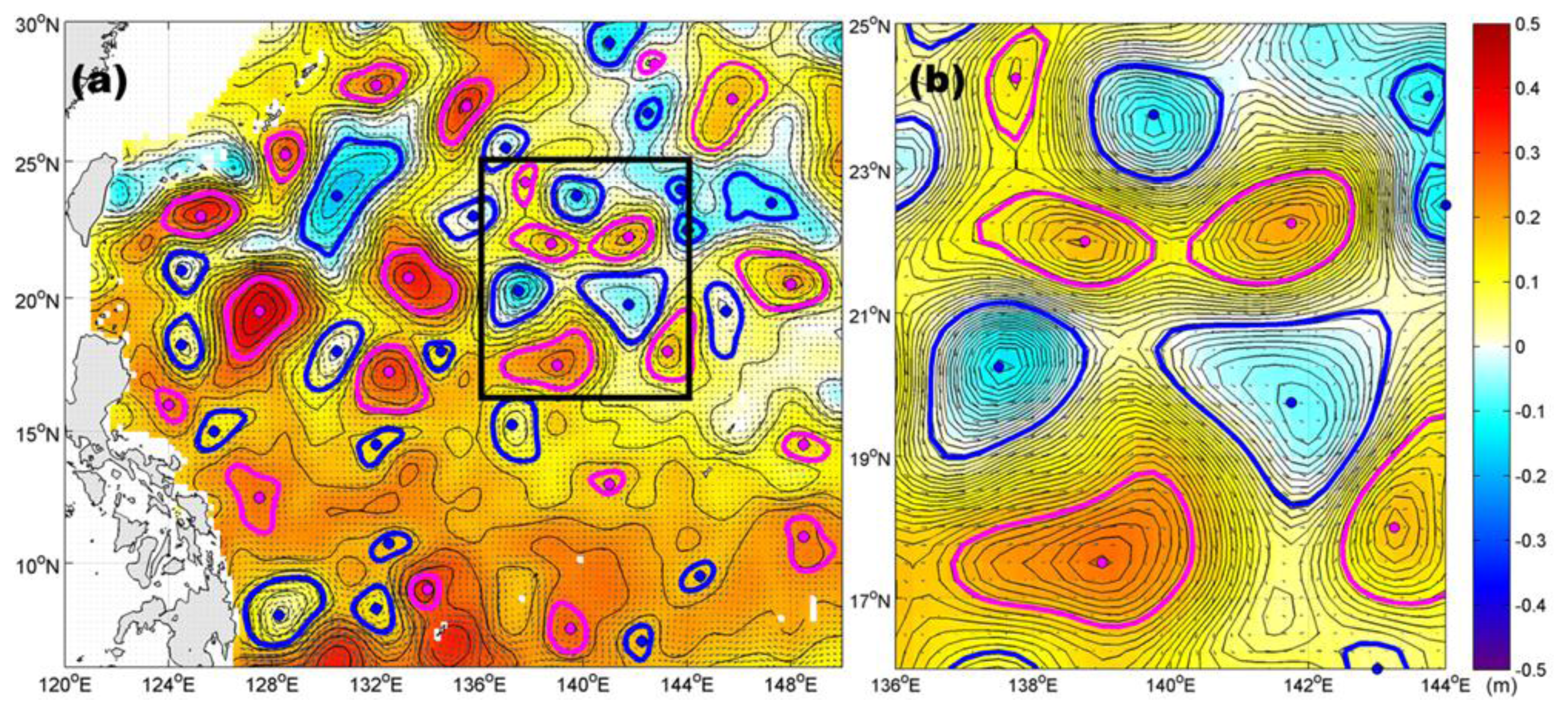
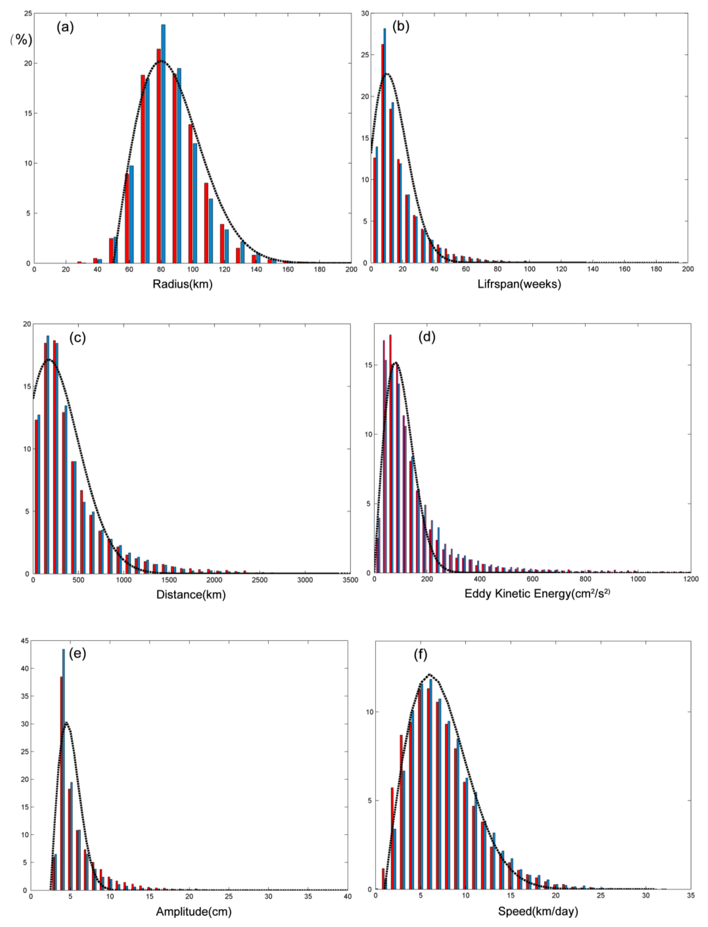
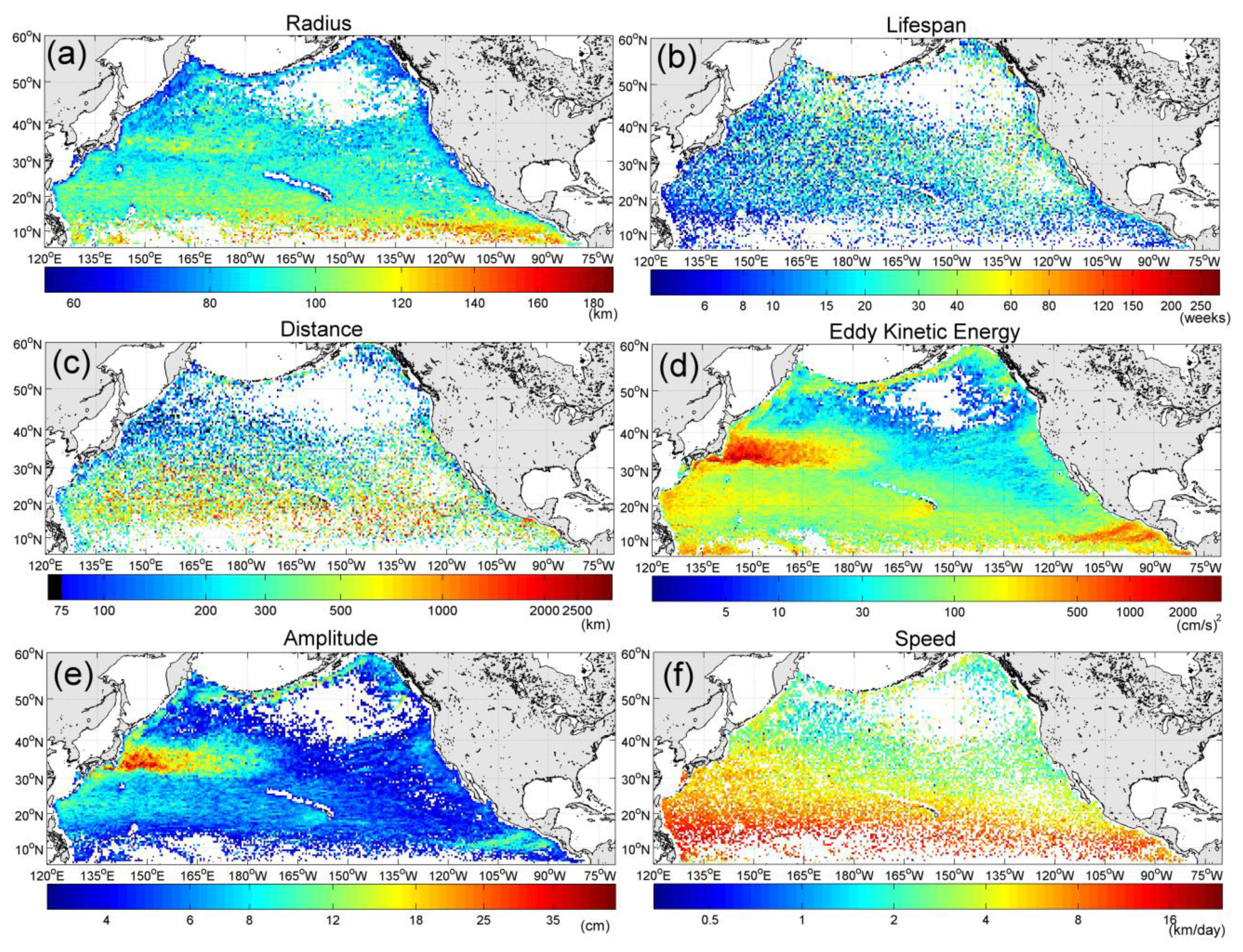
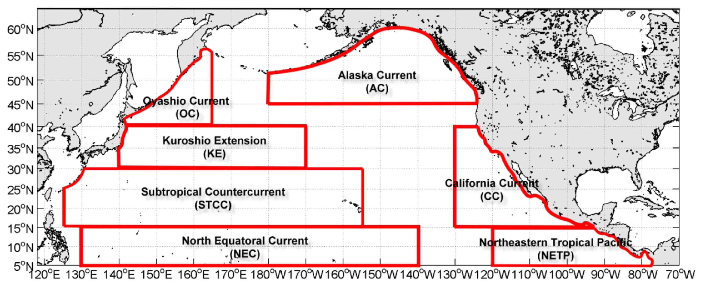
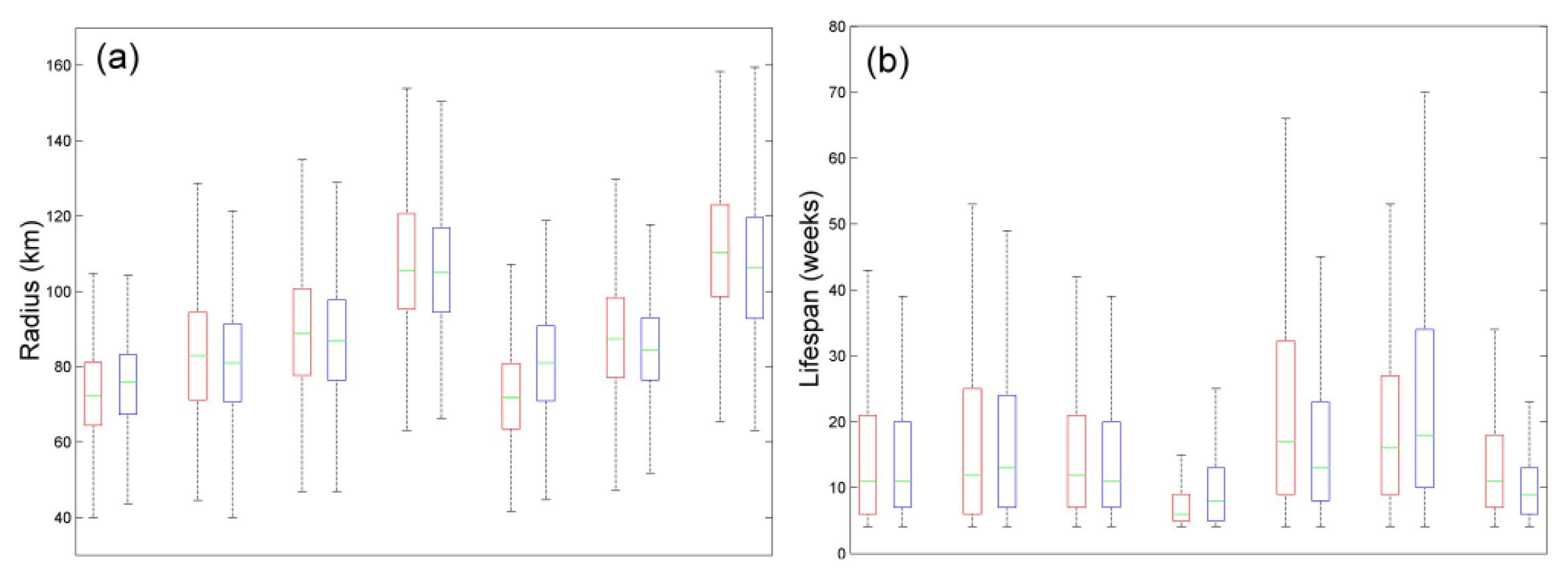
4.1. Statistical Characteristics

This study examines eddies with a lifespan longer than 4 weeks in the North Pacific. The total number of eddies is 19,836, including 10,398 cyclonic eddies and 9438 anticyclonic eddies from October 1992 to December 2012. Figure 3a shows the histogram of eddy radius distribution. One can see that it is close to the Gaussian distribution, but the peak value skews a little toward the smaller size. This result agrees with that in the STCC by Liu et al. [12]. The mean radius value is 86 km for anticyclonic eddies and 85 km for cyclonic eddies. Figure 3b shows the distribution of lifespans. The mean value of lifespan is about 18 weeks, and some eddies are able to survive for a couple of years. Figure 3c shows the distribution of travel distances, which looks like the distribution of lifespans, because eddies with longer lifespans certainly propagate for longer distances. On the other hand, some eddies can have high EKE (>1000 cm2/s2), though the mean value of EKE is about 176 cm2/s2. The kinetic energy of mesoscale eddies in the North Pacific is one order greater than the mean kinetic ocean energy [3,4]. Figure 3 shows the histogram of eddy characteristics in the North Pacific, and we use the probability density function of the Rayleigh distribution to fit them. The results reveal that histograms of radius, propagation speed, amplitude, and eddy kinetic energy are approximated by the Rayleigh distribution.
The eddy characteristics in the North Pacific are displayed in Figure 4. Based on the maps of EKE (Figure 4d) and the amplitude (Figure 4e), the figures show that there are several active regions of eddy, including the Oyashio, the Kuroshio Extension, the STCC, the lee side of Hawaiian Islands, the northeastern tropical Pacific, Californian currents, and Alaskan currents. Using SLA data, Liu et al. [12] showed that the regions of Kuroshio Extension and the STCC were more active with high EKE in the western North Pacific. On the other side, eddies are hardly observed around the center of the eastern part of the North Pacific Subarctic Gyre (discussed in Section 4.2). The radius, travel distance, and speed mainly vary with latitude. At lower latitudes, eddies possess greater radii, speeds, and travel distances. Due to the 25-km spatial resolution of SLA, we assume that travel distances shorter than 75 km are stationary eddies. Figure 4c reveals that most of the eddies in the North Pacific are moving eddies; meanwhile a sporadic distribution of stationary eddies appears at higher latitudes. Chelton et al. [9] indicated that eddy speeds were mainly affected by the phase speed of long baroclinic Rossby waves decreasing with latitude. The speed was smaller than 0.8 km/day at 40°N, thus stationary eddies potentially appear at higher latitudes. Furthermore, seven more active regions in the North Pacific are drawn out and discussed below (Figure 5).
The Kuroshio Extension/Oyashio region encompasses the Kuroshio Extension, the Oyashio, and the Subarctic Current. In this region, eddies can persist from several months to longer than two years. The existence of eddies has a strong influence on the local climate, hydrography, and fishery [30,31]. Qiu et al. [32] indicated that eddies in this region could also affect the North Pacific subtropical mode waters. The behavior of these mesoscale eddies are related to the bottom topography and variability of currents, such as meanders of the Kuroshio Extension, and southward intrusions and the eastward extension of Oyashio [33]. The number of eddies in this region is around 200 per 1° latitude × 1° longitude in the past 20 years. It is more concentrated than in other places in the North Pacific. The average radius of eddies in the Kuroshio Extension and in the Oyashio is 80 km and 70 km, respectively. These results are close to those in the study of Itoh and Yasuda [15].
The lee side of Hawaiian Islands and the STCC region compose the second zonal band with strong eddy activity in the western Pacific [34]. The higher density of number is similar to the Kuroshio Extension region. Qiu [35] suggested that eddies within this region could impact the subtropical gyre. The average size and propagation speed are about 90 km and 8 km/day, which is in agreement with the study of Hwang et al. [14]. In this region, eddies can also persist for longer than one year.
The equatorial current zone is an area with inactivity of eddy and a lack of investigation. A total of 691 cyclonic eddies and 412 anticyclonic eddies have been detected in the last two decades. The number of cyclonic eddy is larger than that of anticyclonic eddy. The phenomenon is different from other regions iwhich the numbers of cyclonic eddies and anticyclonic eddies are similar. Velocity shear between the westward North Equatorial Current and the eastward Equatorial Countercurrent generating positive vorticity could be the reason; hence the number of cyclonic eddies is a little larger than that of anticyclonic eddies. However, further studies are needed in this area. Bauer et al. [36] investigated the eddy-mean flow decomposition in the tropical Pacific and indicated that the eddy energy was about 380 cm2/s2 and the mean radius was 100 km. The lifespan of eddies is a few months, and it is the shortest in the North Pacific.
In the northern Gulf of Alaska region, mesoscale eddies are an important mechanism for cross-shelf exchange [37]. As described in the study of Crawford et al. [38], eddies in this region have radii of around 80 km and can live up to 3 years. In this study we also observe that the average radius of eddies is 74 km and the lifespan could be longer than 3 years. The EKE is about 50 cm2/s2, which is smaller than in other regions. The generation mechanisms of these eddies could be reversals of downwelling winds or the interaction of the Alaska currents with the topography [39].
In the California Current region, the average eddy radius and EKE are about 85 km and 80 cm2/s2, respectively. The propagation speed is about 4 km/day. This region is the third active region of eddies in the North Pacific with an eddy number of 170/degree2. The distance that eddies can propagate ranges from an average of 300 km to more than 1600 km. It is believed that instabilities of the California Current and wind forcing create those energetic mesoscale eddies [40]. Kurian et al. [41] revealed that most eddies had radii within a range of 25–100 km and propagation speeds from 0 to 10 km/day.
The Northeastern Tropical Pacific region is defined as the ocean from 5° to 15°N and from 120°W to the coast of Central America. Palacios and Bograd [42] used a 12-year time series of satellite altimetry data to characterize eddies. They showed that the average eddy lifespan was around 84–143 days and the radius could range from 50 to over 200 km, but cyclonic eddies dissipated more quickly [43].

4.2. Uncertainties and Errors

As described in Section 3.2, the limitations of the eddy detection method used in this study are mainly influenced by the spatial/temporal resolution of SLA. In this study, eddies can only be detected if their diameters and lifespans are greater than 50 km and 7 day, respectively. Moreover, eddies with lifespans longer than 4 weeks are only considered in this study to avoid the risk of spurious eddies that arise by noise in the SLA field. In this section, uncertainties and errors of statistical analysis are discussed. Table 1 shows the mean, standard deviation, and maximum (minimum) value of eddy characteristics in the seven active regions (Figure 5). As can be seen, lifespan, EKE, distance, and amplitude of eddies have large standard deviations. A large standard deviation implies that the values of these characters are more uncertain. Although the mean lifespan at higher latitudes is around 20 weeks, sometimes eddies can live for more than 3 years. As shown in Figure 3, the distributions of eddy kinematic properties in the North Pacific are positively skewed which is indicated by the fact that the tail on the high value side is longer than on the low value side. Because the mean values of lifespan, EKE, distance, and amplitude are not highly significant, they are not indicated for comparing the differences of eddy characters in the seven regions. Therefore, boxplots of eddy kinematics with the 25th and 75th percentile are used to compare the differences (Figure 6). The radius, lifespan, travel distance, and speed are mainly affected by latitude. Although anticyclonic eddies possess greater radii, amplitudes, and lifespans than cyclonic eddies, EKE of cyclonic eddies is not smaller than that of anticyclonic eddies. Compared to other regions, the lifespan of eddies is the greatest, but EKE is the weakest in the Alaska Current region. Moreover, the travel distance of eddies in this region can be greater than 600 km. Ladd et al. [44] also showed that water had been transported for hundreds of kilometers by eddies in the Gulf of Alaska region. The largest amplitude is revealed in the Kuroshio Extension and Northeastern Tropical Pacific regions. The smallest lifespan and amplitude appear in the North Equatorial Current region. Although the greatest EKE in the western North Pacific appears in the Northeastern Tropical Pacific region, the number of eddy in the Northeastern Tropical Pacific region (about 100/degree2) is smaller than that in the California Current region (about 250/degree2) in the last two decades. Eddies in the Kuroshio Extension and the Northeastern Tropical Pacific regions possess a bigger potential to carry water mass and influence the large-scale flux of momentum, heat, and salt, because they possess greater a EKE in those regions.

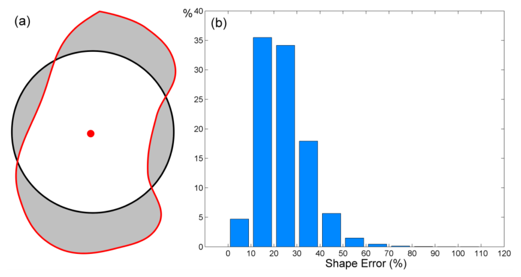
4.3. Shape Error of Eddy

The shape of eddy might be affected by a strong background flow or other eddies, hence the eddy shape would not be as an ideal circle. A test of shape error of eddies detected by the algorithm is discussed in this section. As shown in Figure 7a, closed contours of the eddy edge would have gap and bulge areas within and outside the fitted ideal circle, respectively. Kurian et al. [41] defined the shape error of eddy as the ratio between the area of deviations to the area of the ideal circle. A histogram of the shape error reveals that the eddy detected by the algorithm in the North Pacific is 24% of the mean value with 11% of one standard deviation (Figure 7b). The shape error of less than 50% is account for by 98% of the total eddies in the North Pacific. This implies that the eddy detection algorithm used in this study has successfully reduced the effect of mean flow on eddy shape.

4.4. Eddy Generation and Termination
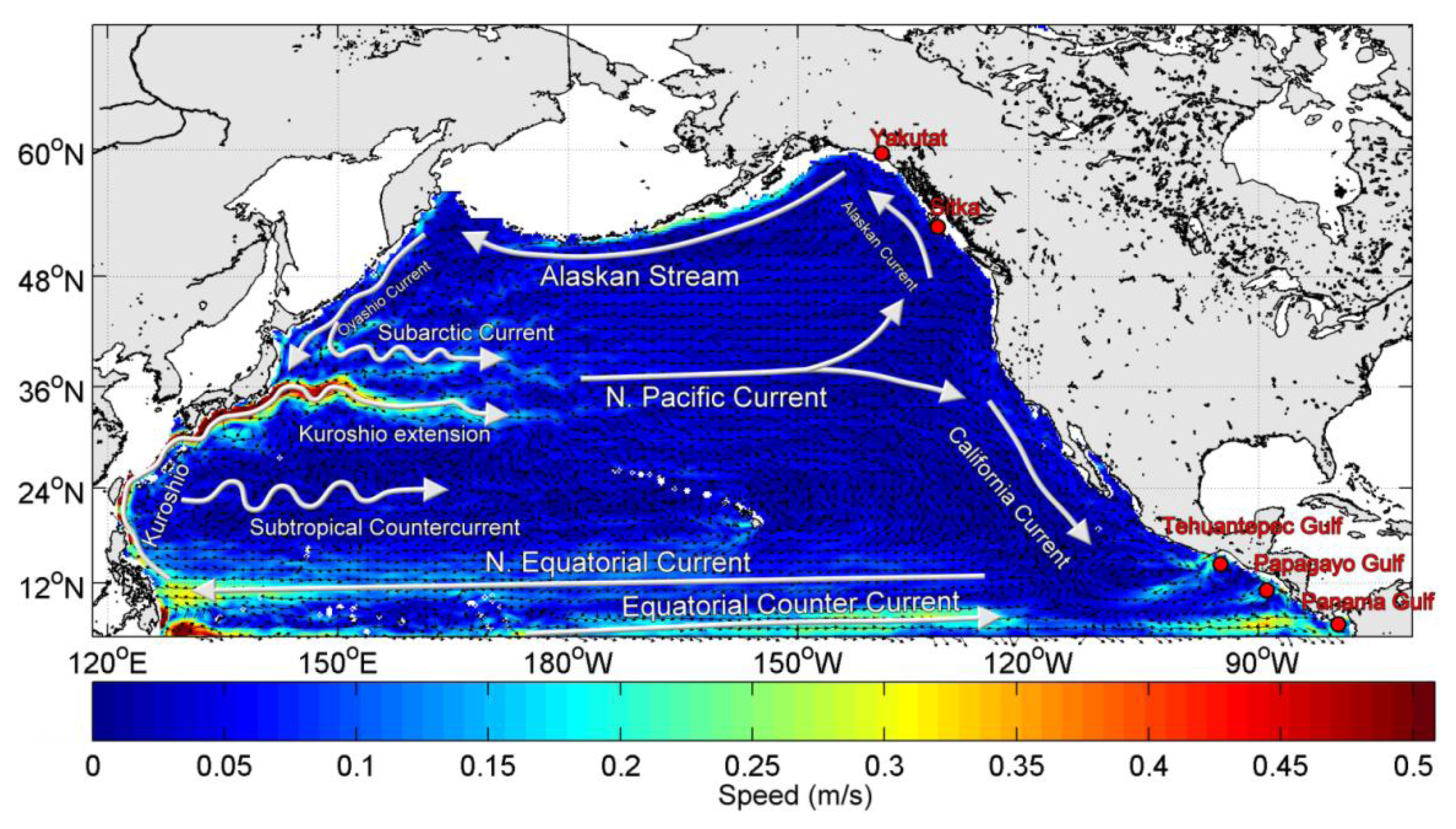
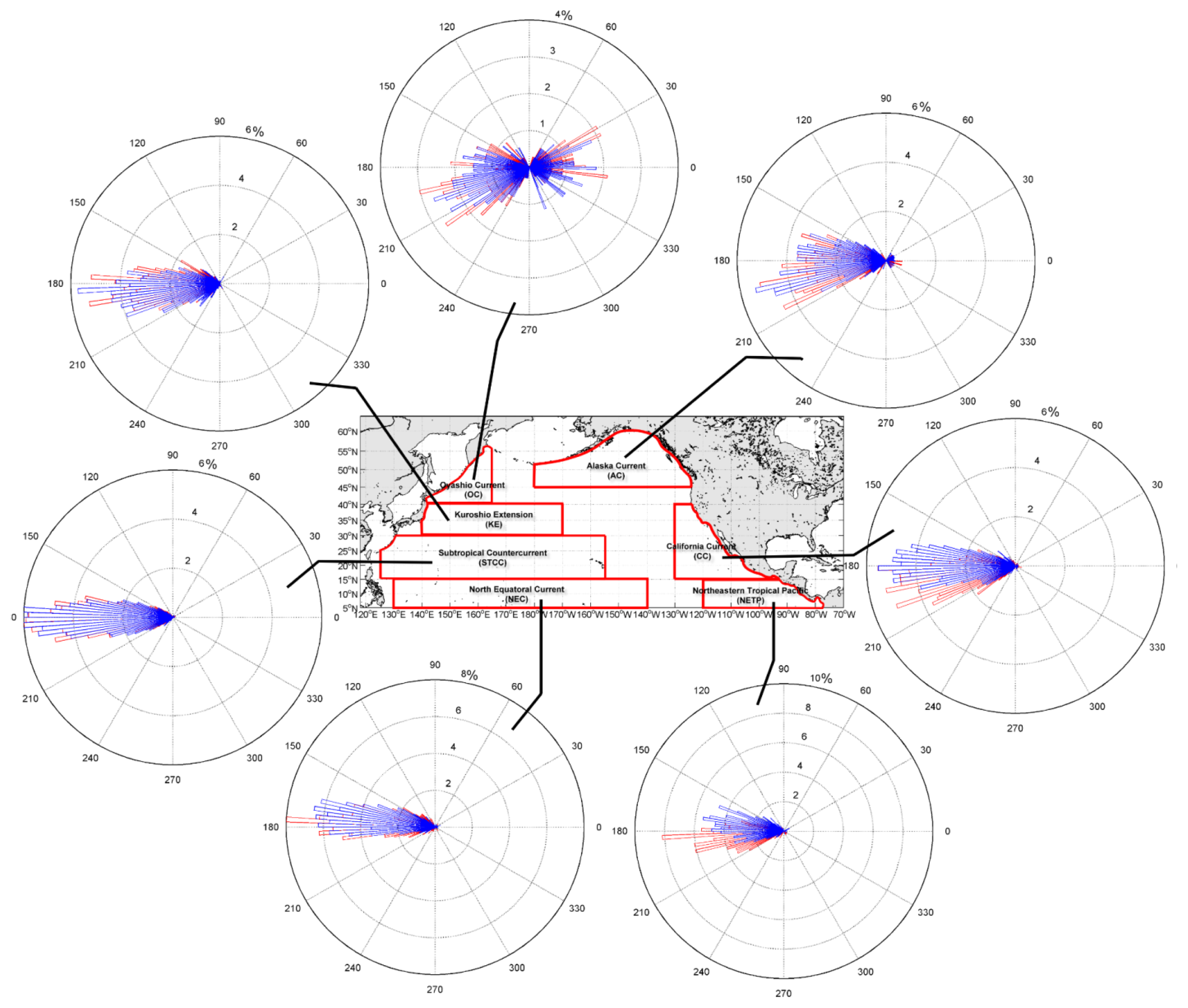
The formation and the termination of eddies are defined by the first and the last record of time series of each eddy lifespan, respectively. Figure 8 shows the spatial distribution of eddy formation and termination. The results indicate that eddies can generate and terminate in most regions, except for the center of the eastern part of the North Pacific Subarctic Gyre. The west coast of North America, the coast of Central America, the Kuroshio Extension, the Oyashio, and the lee side of Hawaiian Islands are the major generation locations. In the Alaska Current region, eddies are often formed near the coast of Yakutat and Sitka [17]. Kurian et al. [41] observed eddies in the California Current system and indicated that many of eddies formed near the coast with high eddy kinetic energy (0.018 m2/s2). In the northeastern tropical Pacific, the ocean is strongly modulated by three powerful wind jets over the Tehuantepec, Papagayo, and Panama Gulfs [45]. Therefore, there are three bands of strong mesoscale eddy variability off the coast of Central America from the Tehuantepec, Papagayo, and Panama Gulfs [42]. Itoh and Yasuda [15] revealed that many eddies were generated along the Kuroshio Extension. Anticyclonic and cyclonic eddies shed off from the northern and southern Kuroshio Extension, respectively. On the lee side of Hawaiian Islands and in the STCC region, eddies are generated by different mechanisms. Qiu [35] suggested that eddies in the STCC region could be generated by the baroclinic instability of the vertical current shear. On the lee side of Hawaiian Islands, eddies are generated mainly due to wind curls and wakes of the Hawaiian Islands [46].
Because of the nearly westward propagation of the eddies, the Kuroshio and the Oyashio currents play a role in terminating eddies [9]. Contrarily, eddies are seldom observed in vast areas around the center of the eastern part of the North Pacific Subarctic Gyre (Figure 8a), because the eddy sizes there are too small to be resolved [8]. From the kinetic energy distribution of currents in the study area derived from altimetry ADT (Figure 9), a relatively small kinetic energy is found in the North Pacific subarctic Gyre. Based on the fact that the formation of eddies requires energy supplies provided by the unstable oceanic kinetics, this may be the reason that eddies rarely form in this region.

4.5. Eddy Path

Chelton et al. [9] revealed that a striking feature of eddy trajectories in global oceans is obviously traveling westward with small deflections. In this study the results of eddy tracking similarly show that eddies propagate westward with various meridional deflections. As shown in Figure 10, we apply the linear regression method to eddy trajectories and define the angle of azimuth in relation to the east direction. The map of eddy azimuth shows that most eddies propagate nearly westward. Nevertheless, eddies propagate southwestward near the coast of eastern Japan and northeastward around the Subarctic Front. Similar results were also found in the study of Itoh and Yasuda [15]. In the Kuroshio Extension and the STCC regions, the trajectories of eddies exhibit a strong westward propagating tendency (180°). Eddies are generated by the frontal instability associated with the STCC and can be carried by the westward propagating Rossby waves [47]. Eddies in the southern Japan region propagate eastward, which means that they may be affected by the strong eastward Kuroshio Extension. Although this region is around the large meander in the Kuroshio south of central Japan, we could detect mesoscale eddies but not the Kuroshio meanders. Near the eastern coast of Taiwan and Luzon, eddies propagating with about 100° azimuth might be affected by the northward Kuroshio. Moreover, Eddies purely propagate along the coast around the Alaska Stream. Eddies are strongly influenced by the Alaskan Stream system in this region. The Gulf of Alaska turns southwestward following the self-break and forms the Alaskan Stream, which may carry eddies [37]. Xiu et al. [48] demonstrated that eddies detached and propagated away from the coast along the Alaskan Stream. On the other hands, the propagation of anticyclonic and cyclonic eddies differs more around the California currents. As noted in previous studies [9,41], eddies show a tendency for westward propagation with cyclonic and anticyclonic eddies exhibiting a poleward and equatorward deflection. This suggests that nonlinear eddy propagation may be influenced by the β-effect and self-advection [49].
Furthermore, circular histograms of the mean azimuth in seven active regions are used to display the difference (Figure 11). Eddies propagate southwestward with 210° and northeastward with 30° nearly parallel to the coastal line of eastern Japan around the Oyashio currents. In the North Equatorial Current region, regardless of whether the eddies are cyclonic or anticyclonic, the northwestward propagation near an 170° azimuth may be affected by the North Equatorial Current. In the Alaska Current region, eddies are strongly influenced by the Alaskan Stream that propagates westward at 208° azimuth for anticyclonic eddies and 203° for cyclonic eddies. The differences of deflection between anticyclonic and cyclonic eddies may be affected by the combined influence of the β effect and the advection effect of the Alaskan Stream. Therefore, the equatorward deflections of anticyclonic eddies are more noticeable than the deflections exhibited by cyclonic eddies. In the regions of the California Current and the Northeastern Tropical Pacific, eddies propagate westward with cyclonic eddies exhibiting a slight deflection toward to the pole (165°); and anticyclonic eddies tending toward to the equator (197°). However, this kind of distribution of the eddy pathways in the other regions is not remarkable. The eddy trajectories may be affected mainly by eddy-eddy and eddy-mean flow interactions. Based on the aforementioned results, the effects of the background current may not be crucial for eddy trajectories around the California currents compared with other regions in the North Pacific.

5. Conclusions

The weekly SLA data derived from satellite altimetry are used to investigate the mesoscale eddies in the North Pacific. To extract eddies from the ocean surface, we use the free-threshold eddy identification algorithm. This study considers eddies with lifespans longer than 4 weeks and investigates their characters. According to results of analyses of the SLA between November 1992 and December 2012, histograms of radius, propagation speed, amplitude, and eddy kinetic energy are approximated by the Rayleigh distribution. From maps of EKE and amplitude, eddies are more active in the regions of Kuroshio Extension, STCC, the lee side of the Hawaiian Islands and the northeastern tropical Pacific. Although eddies can generate and terminate in most regions, eddies are rarely observed around the center of the eastern part of the North Pacific Subarctic Gyre. The radius, travel distance, and speed of eddies mainly decrease with increase in latitude. On the whole, anticyclonic eddies possess greater radii, amplitudes, and lifespans than cyclonic eddies, but the EKE of cyclonic eddies is not smaller than that of anticyclonic eddies. Lifespans of eddies which can live up to 3 years in the Alaska Current region are the greatest in the North Pacific. The largest amplitude and EKE are revealed in the Kuroshio Extension and Northeastern Tropical Pacific regions, hence these regions possess a bigger potential to carry water mass and influence the large-scale flux of momentum, heat, and salt. Regarding of whether the eddies are found in the regions of California Current or the Northeastern Tropical Pacific, most eddies propagate westward with slight equatorward and poleward deflections for cyclonic and anti-cyclonic eddies, respectively. This result suggests that eddy propagation may be influenced by the β-effect. However, this divergence of the eddy pathways is not remarkable in other regions. Around the Oyashio currents, most eddies propagate nearly parallel to the coastal line of eastern Japan. This study gives a statistical analysis and premilinary results of eddies in the North Pacific. Nevertheless, more detailed studies of the dynamic processes and eddy generation mechanisms constitute a challenge for future research.

Acknowledgments

The altimeter products were produced by Ssalto/Duacs and distributed by AVISO, with support from CNES. MSS_CNES_CLS10 and MDT_CNES-CLS09 were produced by CLS Space Oceanography Division and distributed by AVISO, with support from CNES. This work is supported by the National Science Council of Taiwan through grant NSC 102-2611-M-019-011.
  • Author ContributionsYu-Hsin Cheng wrote the most part of this manuscript and worked on data preparation and analysis. Chung-Ru Ho was responsible for research design. Quanan Zheng and Nan-Jung Kuo supported the analysis and interpretation of the results. All of the authors contributed in writing and editing the manuscript.

Conflicts of Interest

The authors declare no conflict of interest.

References

  1. Minobe, S.; Kuwano-Yoshida, A.; Komori, N.; Xie, S.P.; Small, R.J. Influence of the Gulf Stream on the troposphere. Nature 2008, 452, 206–209. [Google Scholar]
  2. Jochum, M.; Danabasoglu, G.; Holland, M.; Kwon, Y.O.; Large, W.G. Ocean viscosity and climate. J. Geophys. Res 2008, 113, C06017. [Google Scholar]
  3. Richardson, P.L. Eddy kinetic energy in the North Atlantic from surface drifters. J. Geophys. Res 1983, 88, 4355–4367. [Google Scholar]
  4. Wyrtki, K.; Magaard, L.; Hager, J. Eddy energy in the oceans. J. Geophys. Res 1976, 81, 2641–2646. [Google Scholar]
  5. Isern-Fontanet, J.; Garcia-Ladona, E.; Font, J. Vortices of the mediterranean sea: An altimetric perspective. J. Phys. Oceanogr 2006, 36, 87–103. [Google Scholar]
  6. Robinson, A.R. Eddies in Marine Science; Springer: New York, NY, USA, 1983. [Google Scholar]Remote Sens 2014, 6, 5181.
  7. Petersen, M.R.; Williams, S.J.; Maltrud, M.E.; Hecht, M.W.; Hamann, B. A three-dimensional eddy census of a high-resolution global ocean simulation. J. Geophys. Res 2013, 118, 1759–1774. [Google Scholar]
  8. Chelton, D.B.; Schlax, M.G.; Samelson, R.M.; de Szoeke, R.A. Global observations of large oceanic eddies. Geophys. Res. Lett 2007, 34, L15606. [Google Scholar]
  9. Chelton, D.B.; Schlax, M.G.; Samelson, R.M. Global observations of nonlinear mesoscale eddies. Prog. Oceanogr 2011, 91, 167–216. [Google Scholar]
  10. Semtner, A.J.; Chervin, R.M. Ocean general circulation from a global eddy-resolving model. J. Geophys. Res 1992, 97, 5493–5550. [Google Scholar]
  11. Qiu, B. Kuroshio and Oyashio Currents; Academic Press: Waltham, MA, USA, 2001. [Google Scholar]
  12. Liu, Y.; Dong, C.; Guan, Y.; Chen, D.; McWilliams, J.; Nencioli, F. Eddy analysis in the subtropical zonal band of the North Pacific Ocean. Deep-Sea Res 2012, 68, 54–67. [Google Scholar]
  13. Yoshida, S.; Qiu, B.; Hacker, P. Low-frequency eddy modulations in the Hawaiian Lee Countercurrent: Observations and connection to the Pacific Decadal Oscillation. J. Geophys. Res 2011, 116. [Google Scholar] [CrossRef]
  14. Hwang, C.; Wu, C.R.; Kao, R. TOPEX/Poseidon observations of mesoscale eddies over the Subtropical Countercurrent: Kinematic characteristics of an anticyclonic eddy and a cyclonic eddy. J. Geophys. Res 2004, 109. [Google Scholar] [CrossRef]
  15. Itoh, S.; Yasuda, I. Characteristics of mesoscale eddies in the kuroshio–oyashio extension region detected from the distribution of the sea surface height anomaly. J. Phys. Oceanogr 2010, 40, 1018–1034. [Google Scholar]
  16. Giese, B.S.; Carton, J.A.; Holl, L.J. Sea level variability in the eastern tropical Pacific as observed by TOPEX and tropical ocean-global atmosphere tropical atmosphere-ocean experiment. J. Geophys. Res 1994, 99, 24739–24748. [Google Scholar]
  17. Ladd, C.; Mordy, C.W.; Kachel, N.B.; Stabeno, P.J. Northern gulf of Alaska eddies and associated anomalies. Deep-Sea Res 2007, 54, 487–509. [Google Scholar]
  18. Frenger, I.; Gruber, N.; Knutti, R.; Münnich, M. Imprint of southern ocean eddies on winds, clouds and rainfall. Nature Geosci 2013, 6, 608–612. [Google Scholar]
  19. Xu, Y.; Fu, L.-L. Global variability of the wavenumber spectrum of oceanic mesoscale turbulence. J. Phys. Oceanogr 2011, 41, 802–809. [Google Scholar]
  20. Ray, R.D. Spectral analysis of highly aliased sea-level signals. J. Geophys. Res 1998, 103, 24991–25003. [Google Scholar]
  21. Nencioli, F.; Dong, C.M.; Dickey, T.; Washburn, L.; McWilliams, J.C. A vector geometry-based eddy detection algorithm and its application to a high-resolution numerical model product and high-frequency radar surface velocities in the southern California Bight. J. Atmos. Ocean. Tech 2010, 27, 564–579. [Google Scholar]
  22. Isern-Fontanet, J.; Font, J.; Garcia-Ladona, E.; Emelianov, M.; Millot, C.; Taupier-Letage, I. Spatial structure of anticyclonic eddies in the Algerian basin (Mediterranean Sea) analyzed using the Okubo-Weiss parameter. Deep-Sea Res 2004, 51, 3009–3028. [Google Scholar]
  23. Okubo, A. Horizontal dispersion of floatable particles in the vicinity of velocity singularities such as convergences. Deep-Sea Res 1970, 17, 445–454. [Google Scholar]
  24. Weiss, J. The dynamics of enstrophy transfer in two-dimensional hydrodynamics. Physica D 1991, 48, 273–294. [Google Scholar]
  25. Isern-Fontanet, J.; Garcia-Ladona, E.; Font, J. Identification of marine eddies from altimetric maps. J. Atmos. Ocean. Tech 2003, 20, 772–778. [Google Scholar]
  26. Pasquero, C.; Provenzale, A.; Babiano, A. Parameterization of dispersion in two-dimensional turbulence. J. Fluid Mech 2001, 439, 279–303. [Google Scholar]
  27. Morrow, R.; Birol, F.; Griffin, D.; Sudre, J. Divergent pathways of cyclonic and anti-cyclonic ocean eddies. Geophys. Res. Lett 2004, 31, L24311. [Google Scholar]
  28. Ducet, N.; Le Traon, P.Y.; Reverdin, G. Global high-resolution mapping of ocean circulation from TOPEX/Poseidon and ERS-1 and-2. J. Geophys. Res 2000, 105, 19477–19498. [Google Scholar]
  29. Tomosada, A. Generation and decay of Kuroshio warm-core rings. Deep-Sea Res 1986, 33, 1475–1486. [Google Scholar]
  30. Sugimoto, T.; Tameishi, H. Warm-core rings, streamers and their role on the fishing ground formation around Japan. Deep-Sea Res. I 1992, 39, S183–S201. [Google Scholar]
  31. Yasuda, I.; Okuda, K.; Hirai, M. Evolution of a Kuroshio warm-core ring—Variability of the hydrographic structure. Deep-Sea Res. I 1992, 39, S131–S161. [Google Scholar]
  32. Qiu, B.; Chen, S.; Hacker, P. Effect of mesoscale eddies on subtropical mode water variability from the Kuroshio Extension System Study (KESS). J. Phys. Oceanogr 2007, 37, 982–1000. [Google Scholar]
  33. Isoguchi, O.; Kawamura, H.; Oka, E. Quasi-stationary jets transporting surface warm waters across the transition zone between the subtropical and the subarctic gyres in the north Pacific. J. Geophys. Res 2006, 111. [Google Scholar] [CrossRef]
  34. Qiu, B.; Chen, S. Interannual variability of the north Pacific subtropical countercurrent and its associated mesoscale eddy field. J. Phys. Oceanogr 2010, 40, 213–225. [Google Scholar]
  35. Qiu, B. Seasonal eddy field modulation of the north Pacific subtropical countercurrent: TOPEX/Poseidon observations and theory. J. Phys. Oceanogr 1999, 29, 2471–2486. [Google Scholar]
  36. Bauer, S.; Swenson, M.S.; Griffa, A.; Mariano, A.J.; Owens, K. Eddy-mean flow decomposition and eddy-diffusivity estimates in the tropical Pacific Ocean: 1. Methodology. J. Geophys. Res 1998, 103, 30855–30871. [Google Scholar]
  37. Ladd, C.; Stabeno, P.; Cokelet, E. A note on cross-shelf exchange in the northern Gulf of Alaska. Deep-Sea Res. II 2005, 52, 667–679. [Google Scholar]
  38. Crawford, W.R.; Cherniawsky, J.Y.; Foreman, M.G. Multi-year meanders and eddies in the Alaskan Stream as observed by TOPEX/Poseidon altimeter. Geophys. Res. Lett 2000, 27, 1025–1028. [Google Scholar]
  39. Thomson, R.E.; Gower, J.F. A basin-scale oceanic instability event in the Gulf of Alaska. J. Geophys. Res 1998, 103, 3033–3040. [Google Scholar]
  40. Marchesiello, P.; McWilliams, J.C.; Shchepetkin, A. Equilibrium structure and dynamics of the California current system. J. Phys. Oceanogr 2003, 33, 753–783. [Google Scholar]
  41. Kurian, J.; Colas, F.; Capet, X.; McWilliams, J.C.; Chelton, D.B. Eddy properties in the California current system. J. Geophys. Res 2011, 116. [Google Scholar] [CrossRef]
  42. Palacios, D.M.; Bograd, S.J. A census of Tehuantepec and Papagayo eddies in the northeastern tropical Pacific. Geophys. Res. Lett 2005, 32. [Google Scholar] [CrossRef]
  43. Gonzalez-Silvera, A.; Santamaria-del-Angel, E.; Millan-Nunez, R.; Manzo-Monroy, H. Satellite observations of mesoscale eddies in the Gulfs of Tehuantepec and Papagayo (Eastern Tropical Pacific). Deep-Sea Res 2004, 51, 587–600. [Google Scholar]
  44. Ladd, C.; Kachel, N.B.; Mordy, C.W.; Stabeno, P.J. Observations from a Yakutat eddy in the northern Gulf of Alaska. J. Geophys. Res 2005, 110. [Google Scholar] [CrossRef]
  45. Liang, J.H.; McWilliams, J.C.; Kurian, J.; Colas, F.; Wang, P.; Uchiyama, Y. Mesoscale variability in the northeastern tropical Pacific: Forcing mechanisms and eddy properties. J. Geophys. Res 2012, 117, C07003. [Google Scholar]
  46. Yoshida, S.; Qiu, B.; Hacker, P. Wind-generated eddy characteristics in the lee of the island of Hawaii. J. Geophys. Res 2010, 115, C03019. [Google Scholar]
  47. Qiu, B.; Chen, S. Concurrent decadal mesoscale eddy modulations in the western north Pacific subtropical gyre. J. Phys. Oceanogr 2013, 43, 344–358. [Google Scholar]
  48. Xiu, P.; Chai, F.; Xue, H.J.; Shi, L.; Chao, Y. Modeling the mesoscale eddy field in the Gulf of Alaska. Deep-Sea Res 2012, 63, 102–117. [Google Scholar]
  49. Cushman-Roisin, B.; Tang, B.; Chassignet, E.P. Westward motion of mesoscale eddies. J. Phys. Oceanogr 1990, 20, 758–768. [Google Scholar]
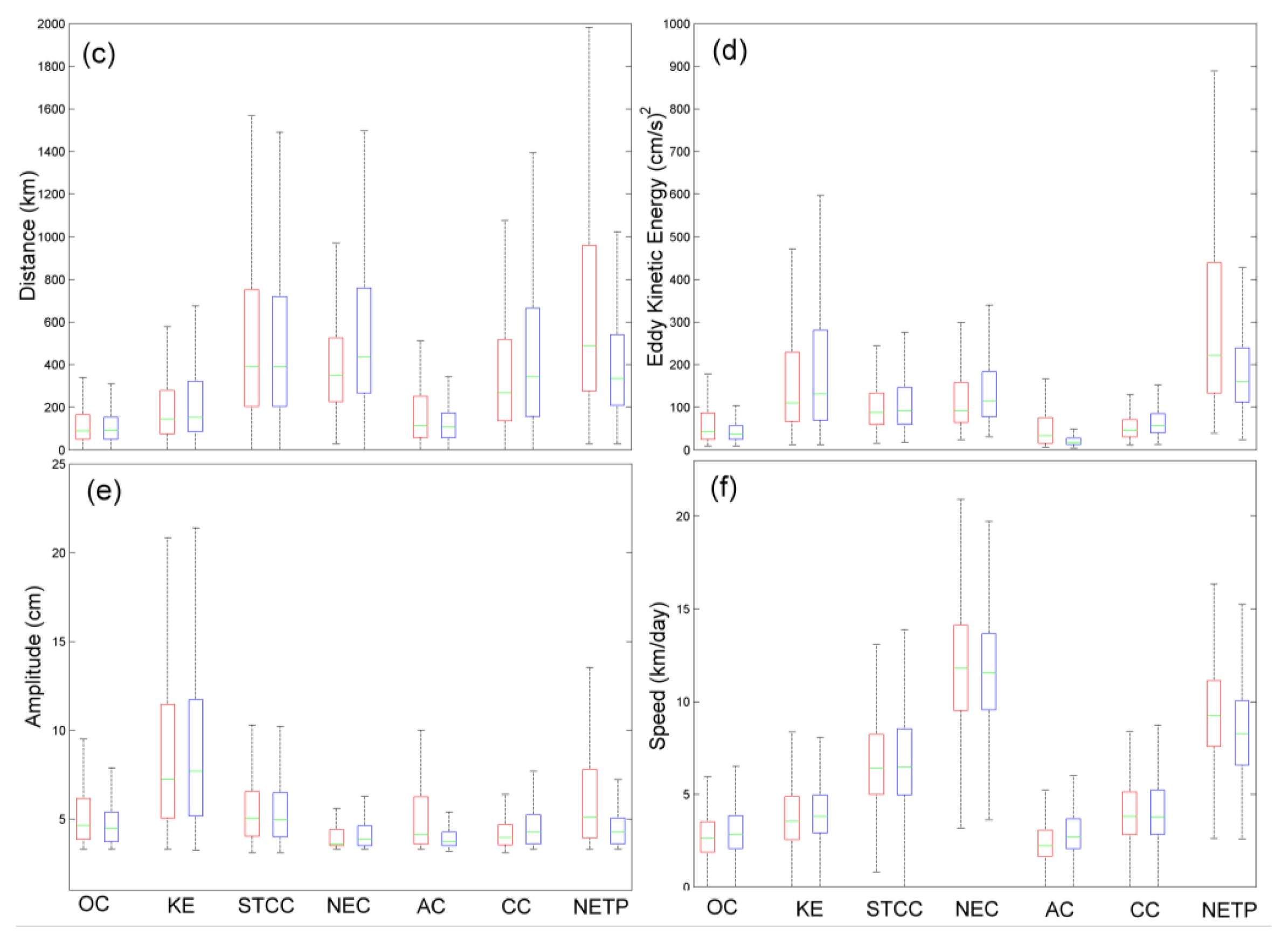
Figure 1. Schematic current patterns in the North Pacific. Geostrophic currents are calculated from altimeter absolute dynamic topography data and averaged over a period from 1992 to 2012. Background color is the speed of geostrophic currents.
Remotesensing 06 05164f1
Figure 2. Sea level anomaly (SLA) and eddies on 14 July 2010. Red and blue dots are the centers of anticyclonic and cyclonic eddies, respectively. The eddy edges are enclosed by red (blue) lines. (a) Continuous contour lines are displayed every 4 cm; (b) Zoom in of the region of black box in (a). Continuous contour lines are displayed every 1 cm.
Remotesensing 06 05164f2
Figure 3. Histogram of eddy radius (a); lifespan (b); travel distance (c); eddy kinetic energy (EKE) (d); amplitude (e); and speed (f). Red and blue bars stand for anticyclonic and cyclonic eddies, respectively. The dotted line is the fitting line of a Rayleigh distribution.
Remotesensing 06 05164f3
Figure 4. Maps of eddy radius (a); lifespan (b); travel distance (c); EKE (d); amplitude (e); and speed (f).
Remotesensing 06 05164f4
Figure 5. Map of active regions in the North Pacific.
Remotesensing 06 05164f5
Figure 6. Boxplot of eddy kinematic characteristics in the active regions in Figure 5. The green line is the median value and the box represents the interquartile range. The whiskers are lines extending from each end of the box to show the extent of the rest of the data. The whiskers’ length is 1.5 times that of the interquartile range. If all data lie within the area of 1.5 times the interquartile range, the whiskers end with the minimum or maximum of the data. (a) Radius; (b) Lifespan; (c) Distance; (d) EKE; (e) Amplitude; (f) Speed. Red and blue represent the anticyclonic and cyclonic eddies, respectively.
Remotesensing 06 05164f6aRemotesensing 06 05164f6b
Figure 7. Sketch (a) and histogram (b) of shape error. The closed contour of the eddy edge and the ideal circle are represented by the red and black lines, respectively. Area deviations are the sum of the shaded regions, and the shape area is the area deviation expressed as the percentage of the area of the fitted circle.
Remotesensing 06 05164f7
Figure 8. Statistics for eddies with lifespan more than or equal to 4 weeks showing the numbers of (a) eddy generations and (b) eddy terminations for each 1° × 1° region over a 20-year period.
Remotesensing 06 05164f8
Figure 9. Spatial distribution of kinetic energy in the North Pacific calculated from altimeter absolute dynamic topography (ADT) data and averaged over the 20-year period.
Remotesensing 06 05164f9
Figure 10. The maps of the mean azimuth relative to the eastern anticyclonic (a) and cyclonic eddies (b).
Remotesensing 06 05164f10
Figure 11. The propagation characteristics of cyclonic (blue) and anticyclonic eddies (red) with lifespans longer than or equal to 4 weeks. Circular histogram of the mean azimuth relative to the east in seven active regions in Figure 5.
Remotesensing 06 05164f11
Table 1. Statistics of eddy kinematic properties in seven regions of the North Pacific a from 1992 to 2012 (Mean ± One Standard Deviation).
CharacterNumberDiameter (km)Lifespan (week)EKE (cm2/s2)Distance (km)Amplitude (cm)Speed (km/day)

Region
OCanticyclonic541146 ± 24 (70, 232)18 ± 21 (4, 221)74 ± 76 (8, 449)123 ± 104 (0, 889)6 ± 2 (3, 18)3 ± 1 (0, 12)
cyclonic569152 ± 22 (84, 248)16 ± 15 (4, 122)46 ± 32 (8, 297)116 ± 88 (0, 552)5 ± 1 (3, 14)3 ± 1 (0, 9)

KEanticyclonic1391168 ± 32 (90, 282)19 ± 21 (4, 287)215 ± 262 (12, 1999)237 ± 290 (0, 3831)9 ± 6 (3, 46)4 ± 1 (0, 15)
cyclonic1505162 ± 28 (80, 268)18 ± 16 (4, 163)282 ± 426 (11, 3867)269 ± 335 (0, 3649)10 ± 7 (3, 48)4 ± 1 (0, 10)

STCCanticyclonic2957180 ± 32 (94, 344)17 ± 14 (4, 130)107 ± 69 (15, 817)592 ± 604 (0, 5734)6 ± 2 (3, 19)7 ± 2 (0, 18)
cyclonic3446174 ± 30 (94, 312)15 ± 12 (4, 151)121 ± 107 (17, 2630)542 ± 499 (0, 4679)6 ± 2 (3, 49)7 ± 2 (0, 19)

NECanticyclonic412216 ± 36 (126, 364)7 ± 4 (4, 31)133 ± 111 (24, 832)416 ± 278 (27, 2066)4 ± 1 (3, 8)12 ± 3 (1, 21)
cyclonic691212 ± 34 (132, 362)10 ± 9 (4, 112)148 ± 108 (31, 1133)612 ± 577 (0, 4989)4 ± 1 (3, 17)12 ± 3 (1, 23)

ACanticyclonic457146 ± 24 (82, 220)27 ± 30 (4, 187)61 ± 73 (6, 463)204 ± 241 (0, 1771)5 ± 2 (3, 19)3 ± 1 (0, 10)
cyclonic415164 ± 28 (90, 298)18 ± 13 (4, 94)23 ± 13 (4, 76)140 ± 124 (0, 1018)4 ± 1 (3, 7)3 ± 1 (0, 8)

CCanticyclonic900176 ± 32 (86, 294)22 ± 19 (4, 135)70 ± 109 (10, 1135)423 ± 467 (0, 3545)4 ± 1 (3, 18)4 ± 1 (0, 13)
cyclonic965170 ± 28 (94, 302)25 ± 19 (4, 130)70 ± 44 (13, 452)481 ± 464 (0, 5407)5 ± 1 (3, 11)4 ± 1 (0, 12)

NETPanticyclonic390222 ± 36 (130, 320)14 ± 9 (4, 64)336 ± 294 (39, 1498)743 ± 704 (27, 4816)6 ± 3 (3, 18)9 ± 2 (2, 19)
cyclonic492214 ± 38 (126, 344)10 ± 6 (4, 68)190 ± 117 (24, 910)418 ± 314 (27, 2219)5 ± 1 (3, 11)9 ± 2 (1, 20)
aMinimum and maximum values are in brackets.

