On the Semi-Automatic Retrieval of Biophysical Parameters Based on Spectral Index Optimization

Abstract

Regression models based on spectral indices are typically empirical formulae enabling the mapping of biophysical parameters derived from Earth Observation (EO) data. Due to its empirical nature, it remains nevertheless uncertain to what extent a selected regression model is the most appropriate one, until all band combinations and curve fitting functions are assessed. This paper describes the application of a Spectral Index (SI) assessment toolbox in the Automated Radiative Transfer Models Operator (ARTMO) package. ARTMO enables semi-automatic retrieval and mapping of biophysical parameters from optical remote sensing observations. The SI toolbox facilitates the assessment of biophysical parameter retrieval accuracy of established as well as new and generic SIs. For instance, based on the SI formulation used, all possible band combinations of formulations with up to ten bands can be defined and evaluated. Several options are available in the SI assessment: calibration/validation data partitioning, the addition of noise and the definition of curve fitting models. To illustrate its functioning, all two-band combinations according to simple ratio (SR) and normalized difference (ND) formulations as well as various fitting functions (linear, exponential, power, logarithmic, polynomial) have been assessed. HyMap imaging spectrometer (430–2490 nm) data obtained during the SPARC-2003 campaign in Barrax, Spain, have been used to extract leaf area index (LAI) and leaf chlorophyll content (LCC) estimates. For both SR and ND formulations the most sensitive regions have been identified for two-band combinations of green (539–570 nm) with longwave SWIR (2421–2453 nm) for LAI (r²: 0.83) and far-red (692 nm) with NIR (1340 nm) or shortwave SWIR (1661–1686 nm) for LCC (r²: 0.93). Polynomial, logarithmic and linear fitting functions led to similar best correlations, though spatial differences emerged when applying the functions to HyMap imagery. We suggest that a systematic SI assessment is a strong requirement in the quality assurance approach for accurate biophysical parameter retrieval.

1. Introduction

Quantitative and spatially-explicit retrieval of vegetation biophysical parameters is a requirement in a variety of ecological and agricultural applications. Earth observing (EO) satellites, endowed with a high temporal resolution, enable the retrieval and hence monitoring of plant biophysical parameters [1–3]. With the forthcoming super-spectral Copernicus’ Sentinel-2 [4] and Sentinel-3 missions [5] as well as the planned EnMAP [6], HyspIRI [7] and PRISMA [8] imaging spectrometer missions, an unprecedented data stream becomes available. This data influx requires processing techniques, which are reproducible, accurate and fast, when the retrieval of information on plant growth and health status is envisaged. Typically, the retrieval of biophysical parameters using EO data implies the use of a model [9], which can be either statistical or physical in nature. A statistical regression model enables the linkage of EO data with biophysical parameters of interest [10] by making use of (in situ) calibration data. On the other hand, physically-based approaches allow the retrieval of biophysical parameters by inversion of a radiative transfer model (RTM) against EO data [11,12].

Although inversion of a RTM is generally applicable for a wide range of land cover types and sensor configurations [13], the approach is more often than not computationally demanding. It usually requires auxiliary information to enable the parameterization of the physical model and the description of the boundary conditions for which the model is valid [14,15]. This information may not always be available. Moreover, by introducing input parameter uncertainties, the likelihood increases that model inversion may lead to multiple instead of singular solutions in the soil-vegetation-atmosphere matrices (unified theorem of Hadamard well-posedness). In that case, extra steps are required to overcome the ill-posed problem [16].

Conversely, statistical models are more easily implementable for parameter retrieval and mapping applications. The basic principle is to correlate mathematical combinations of measured reflectances for different wavelength ranges or broad spectral bands with biophysical vegetation parameters of interest (e.g., leaf area index (LAI), leaf chlorophyll content (LCC), fractional vegetation cover) using a fitting function. This procedure can be considered as an empirical spectral index (SI) modelling approach. Over the past four decades, a large number of SI models has been developed for the retrieval of biophysical parameters [9,17,18]. The majority of these SIs and their relationship with biophysical parameters of interest has been developed based on experimental work [19–21].

While being successful for many application cases, the empirical approach suffers from drawbacks as well. Typically, a limited portability to different measurement conditions or sensor characteristics can be noted [22]. Moreover, the approach is sensitive to perturbing factors such as atmospheric conditions, canopy characteristics and differences in viewing or solar position geometry [23,24]. In an attempt to generate more generic relationships, RTM-based dataset simulations have been used to assess for the most sensitive SIs [18,25–29]. A spectral index can quite often be used as an estimator for a biophysical parameter using a fitting function through the data; usually by simple linear regression, but also exponential, power, logarithmic and polynomial fitting functions, among others, are commonly applied [22,30,31]. In statistics, this approach can be categorized as a parametric regression modeling approach. This type of model is determined by the introduction of various properties to obtain formulations linking spectral reflectance with the biophysical parameter of interest. In fact, properties that determine the SI regression function can be defined at three levels:

• Band selection: Typically, most SIs are mathematical formulations consisting of two or three sensor spectral bands (B). How then, do we evaluate with a high enough scrutiny, whether the most sensitive spectral bands—with respect to biophysical parameter retrieval—have been selected? This question is especially relevant in view of the high number of bands associated with imaging spectrometry [32];
• SI formulation: Typically, the normalized difference (ND) formulation is applied, i.e., (B₂ − B₁)/(B₂ + B₁). But again, how do we assess, whether the applied ND formulation is the most accurate one with respect to biophysical parameter retrieval? Even given high spectral resolution multi- or hyperspectral reflectance data, there is no reason to assume that a two-band SI formulation leads to the most accurate empirical relationship [33];
• Fitting function: A regression model is typically reduced to a linear fitting exercise, directly or indirectly by prior transformation to linearity. Also here, the question is, whether the regression function selected is the most accurate one? Typically, saturation effects are common for dense canopies [14,15].

Accordingly, it is uncertain whether an established SI—many have been published in the remote sensing literature—will lead to the most accurate biophysical parameter retrieval, particularly when applied to hyperspectral EO data. To ensure that the most sensitive SI regression model is selected for a specific application, a systematic as well as consistent assessment of an exhaustive set of possible band combinations, SI formulations and curve fitting procedures may be required prior to the selection of an SI model for the retrieval of biophysical parameters from (hyperspectral) EO imagery.

Evidently, this is not a trivial task. In view of forthcoming imaging spectrometers, and to obtain an optimized SI model for biophysical parameter retrieval, the assessment of a large number of band combinations is required. To this end, the requirement for a graphical user interface (GUI) toolbox, assisting EO users in the tedious job of evaluating large sets of SI models, is not a luxury. This observation brings us to the following objectives: (1) To develop an “SI assessment toolbox” for the semi-automatic retrieval of biophysical parameters; (2) To enable a robust assessment procedure to estimate the impact of different index formulations, spectral band settings and curve fitting functions with respect to their capability of biophysical parameter retrieval; and (3) To apply the most accurate SI regression model, to extract biophysical parameters from EO imagery.

Since spectral indices and their associated regression models can either be developed based on experimental or simulated data, both options should be present in an SI assessment module. To this end, the SI toolbox has been developed within the ARTMO (Automated Radiative Transfer Models Operator) modeling environment. The experimental dataset used for testing has been acquired from ESA’s SPARC campaign (Barrax, Spain).

In the following sections, the most recent version of the ARTMO modeling environment will be briefly described. Subsequently, an introduction to the most important components of the SI assessment toolbox will follow. The dataset used is described and finally, an assessment of selected SIs will be presented. A discussion section is devoted to newly developed spectral indices and a conclusion section finalizes this paper.

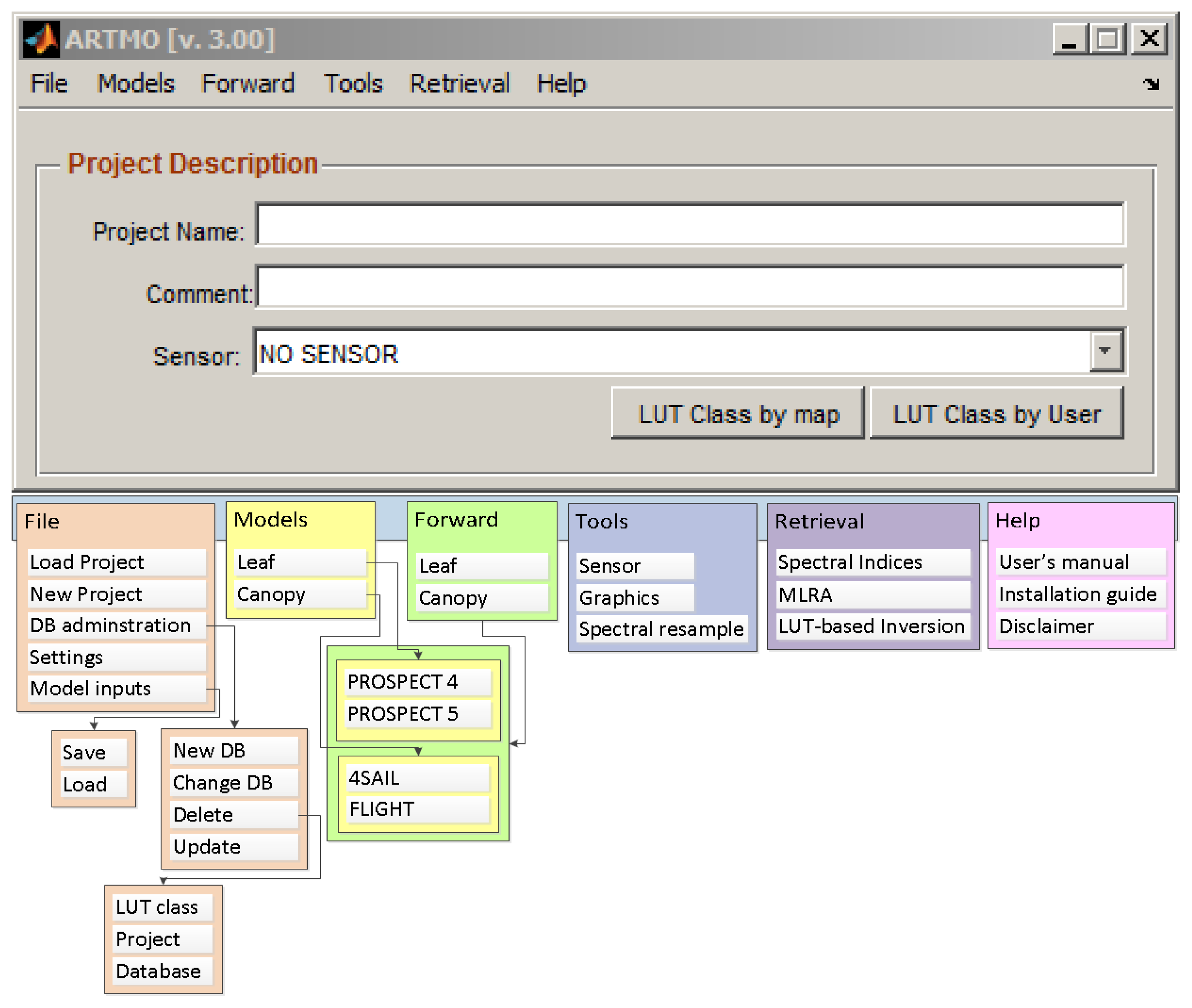
2. ARTMO Software Package

ARTMO, developed and running in Matlab (2011a or higher, The MathWorks, Inc., Natick, MA, USA) on aWindows operating system, offers multiple leaf and canopy radiative transfer models (RTMs) accessible in a GUI environment. Dedicated retrieval methods, required for the semi-automatic retrieval of biophysical parameters, are provided. Examples of ARTMO run options are:

• Selection of various forward and invertible leaf and canopy RTMs of a low to high complexity; leaf: PROSPECT-4 and PROSPECT-5 [34], DLM [35]; canopy: 4SAIL [36], FLIGHT [37]. See also [38] and [39] for more info about RTMs;
• The choice to specify or select spectral band settings specifically for various existing air- and space-borne sensors or user defined settings, typically for recently developed or future sensor systems;
• The option to simulate large datasets of top-of-canopy (TOC) reflectance spectra for sensors sensitive in the optical range (400 to 2500 nm). Look-up tables (LUT) can be generated, which are stored in a relational SQL database management system;
• Finally, various retrieval scenarios can be selected and run using EO reflectance datasets.

Figure 1 illustrates the ARTMO v3 GUI main window and a systematic overview of the modules. In the GUIs main window, a new project can be defined, a sensor chosen and comments added. All processing modules are accessible by drop-down menus from the top bar. Already in the first version of ARTMO, LUT-based inversion applications were available [12,13,40]. ARTMO has been extended since then and v3 is formally presented in this paper. The software package, as well its manuals, installation guides and tutorials, are freely downloadable at [39]. Its most important novelties are briefly listed below:

• ARTMO v3 is designed modularly. Its modular architecture offers the possibility for easy addition (or removal) of components, such as RTM models and post-processing modules;
• The MySQL database is organized in such a way that it supports the modular architecture of ARTMO v3. This avoids redundancy and increases the processing speed. For instance, all spectral datasets are stored as binary objects;
• New retrieval toolboxes are incorporated. They are based on parametric and non-parametric regression as well as physically-based inversion using a LUT. This has led to the development of a: (1) “Spectral Indices assessment toolbox”; (2) “Machine Learning Regression Algorithm toolbox” [41]; and (3) “LUT-based inversion toolbox” [12].

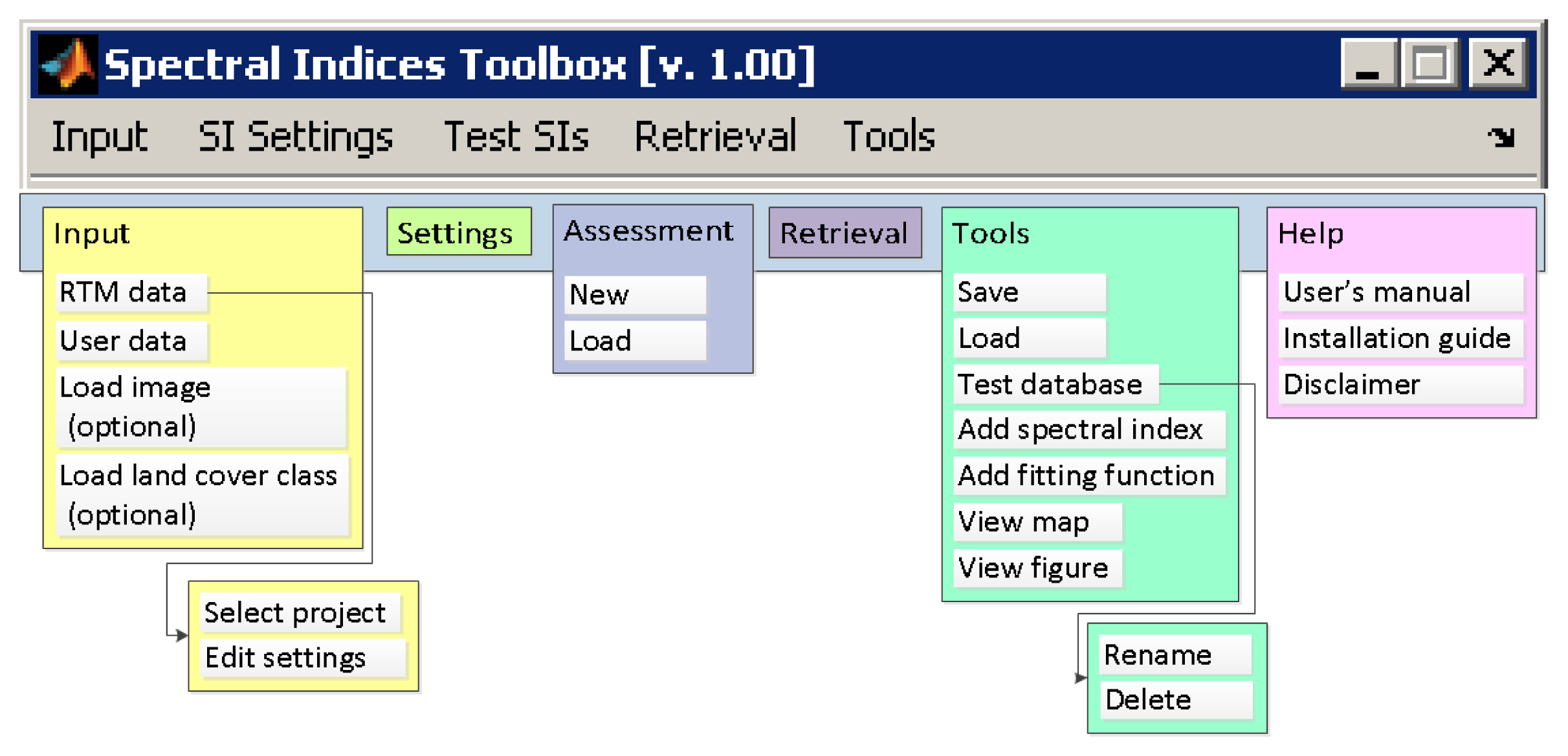
2.1. ARTMO Spectral Indices (SI) Toolbox

This paper introduces a “Spectral Indices assessment toolbox”. Its general architecture is outlined in Figure 2. The toolbox enables the loading and applying of existing or user-defined spectral indices. In short, the toolbox encompasses the following utilities. For each new index, a spectral region for each waveband is specified. Every single band of a sensor that falls within the specified spectral region will then be included in the retrieval capacity assessment. Different types of curve fitting functions have been implemented (e.g., linear, power, exponential, logarithmic, polynomial functions), while new functions can easily be added by the user. Input data originating from RTM runs can be used or user-defined input data can be imported (a plain text file), typically a dataset acquired during a field or flight campaign (i.e., biophysical parameters and associated surface reflectance). Input data can then be partitioned for calibration and validation of the SI–biophysical parameter relationships. Options are available to merge or partition different input datasets; e.g., calibration on the basis of RTM data and validation on the basis of user acquired field data. A land cover map in ENVI format (Exelis Inc., Rochester, NY, USA) can be loaded, which allows that for each land cover class distinct SI optimization strategies can be defined (e.g., vegetation indices for vegetated surfaces, water indices for water bodies, etc.). When validation data are available, a large diversity of spectral band combinations as well as regression functions, can be assessed using the validation dataset and statistical analysis results (see section II-D). The most accurate strategy can then be selected, loaded and applied to retrieve biophysical parameters from EO imagery (in ENVI band-sequential (BSQ) format). Important steps in the outlined procedures are presented in the following sections, they are: (1) “Add spectral index”; (2) “SI settings”; (3) “Calibration/validation assessment”; and (4) “Retrieval”.

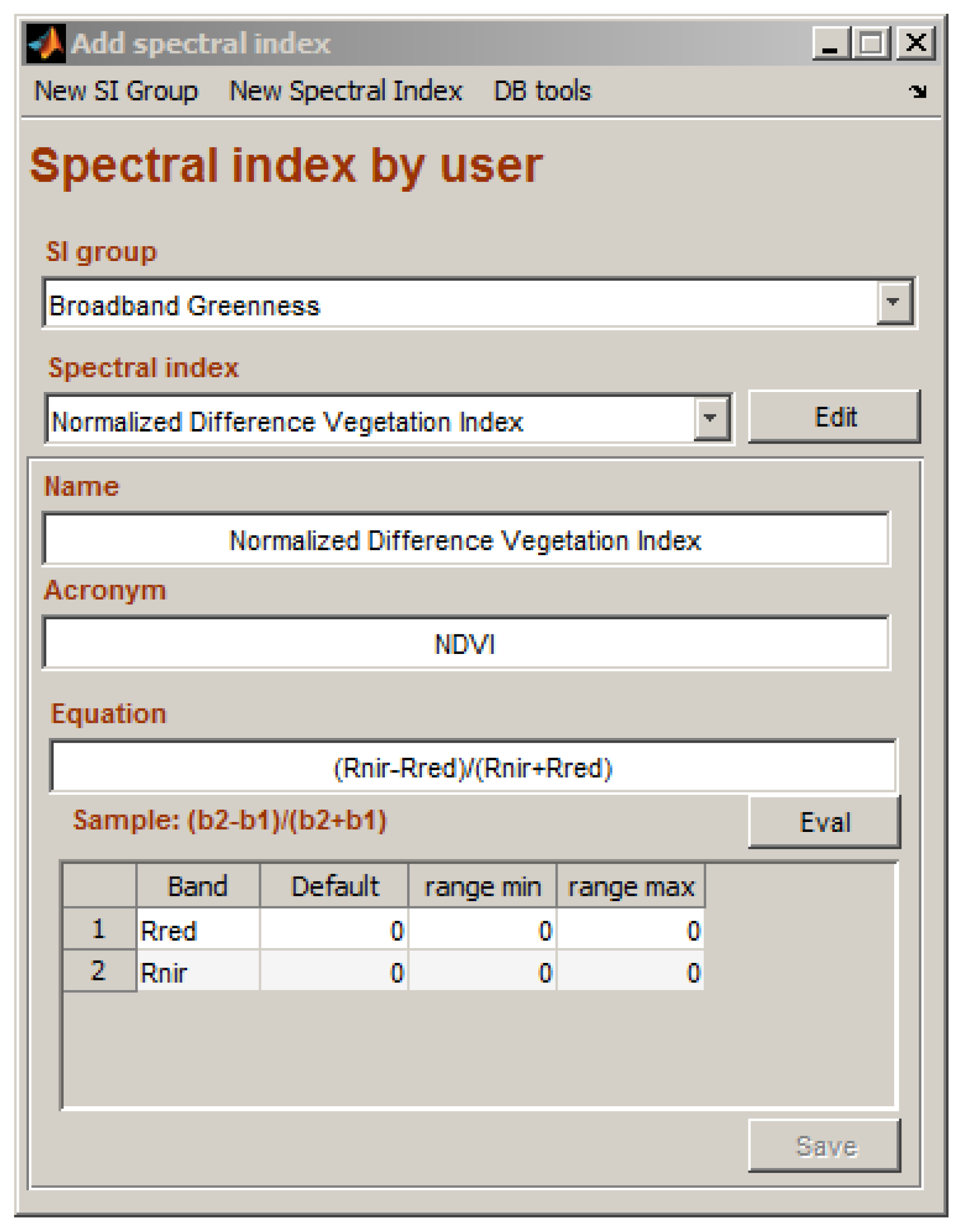
2.2. Add Spectral Index

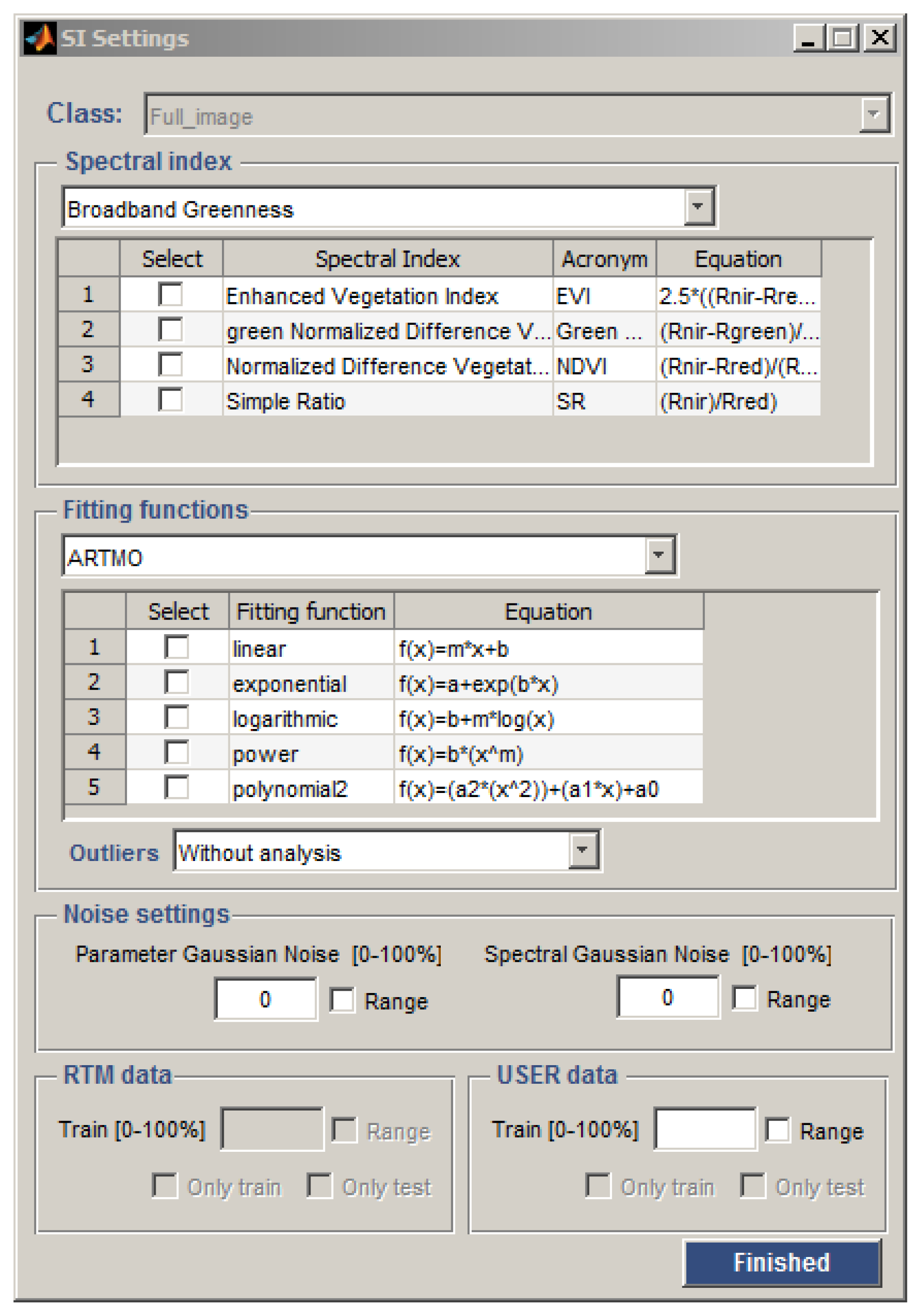
The “Add spectral index” window (Figure 3) in the “Tools” menu allows for adding a new index to a list with pre-defined SIs. Spectral indices can be created manually using the GUI or they may be imported. SIs are organized in “SI Groups”, according to their similarity in definition, e.g., broadband, narrowband or according to their sensitivity with respect to certain absorption features, e.g., by pigments or water. For instance, the “Broadband Greenness” SI group consists of the conventional simple ratio (SR: B₂/B₁) and ND (B₂ − B₁/B₂ + B₁) formulations. A new SI group can also be created, in which multiple SI formulations can be incorporated according to specific input requirements; name, acronym and SI equation definition. When this step is completed, the transfer equation will be assessed for its validity and spectral bands are identified. For each spectral band, a default wavelength or a minimum and maximum of a wavelength range must be specified. During the subsequent assessment step, all bands within the prespecified spectral region will be automatically evaluated. When kept undefined, every single band of a given sensor will be evaluated according to the specified SI formulation.

2.3. SI Settings

In order to activate the possibility of defining SI settings, input data are required. Insertion of input data is performed with the “Input” window. Input data can either consist of a RTM simulated dataset or it can be a field campaign dataset in combination with an EO dataset acquired during the field campaign. The “Input” GUI helps to perform the data selection steps and checks, if data input is correct (GUI not shown for sake of brevity; consult SI toolbox manual at [39]). Subsequently, the SI settings configure the parametric SI models according to various specifications, which are given in the “SI settings” GUI (see Figure 4). First, if multiple land cover types have been pre-defined (using the GUI’s “Load Image and Class” windows), retrieval strategies can be configured specifically for each land cover class. Second, an SI group must be selected so that its encompassing SIs are subsequently listed. From this list, multiple SIs can be selected for assessment purposes. Third, several pre-defined curve fitting functions can be selected for assessment. Fourth, the option to add Gaussian noise is provided, which is useful for the assessment of environmental as well as instrumental uncertainty estimations. The noise function can be applied both for the parameters to be retrieved, as well as on the reflectance spectra used in the assessment. A range of Gaussian noise levels can be specified; hence multiple noise scenarios can be assessed with respect to their impact on retrieval accuracy. Fifth, the calibration/validation (cal/val) data partitioning can be defined according to proportional assignment of data to either calibration or validation (i.e., split-sample approach). Both, field and RTM datasets can be combined by assigning a proportion of each either to calibration or validation. Multiple cal/val partitions can be applied in the assessment.

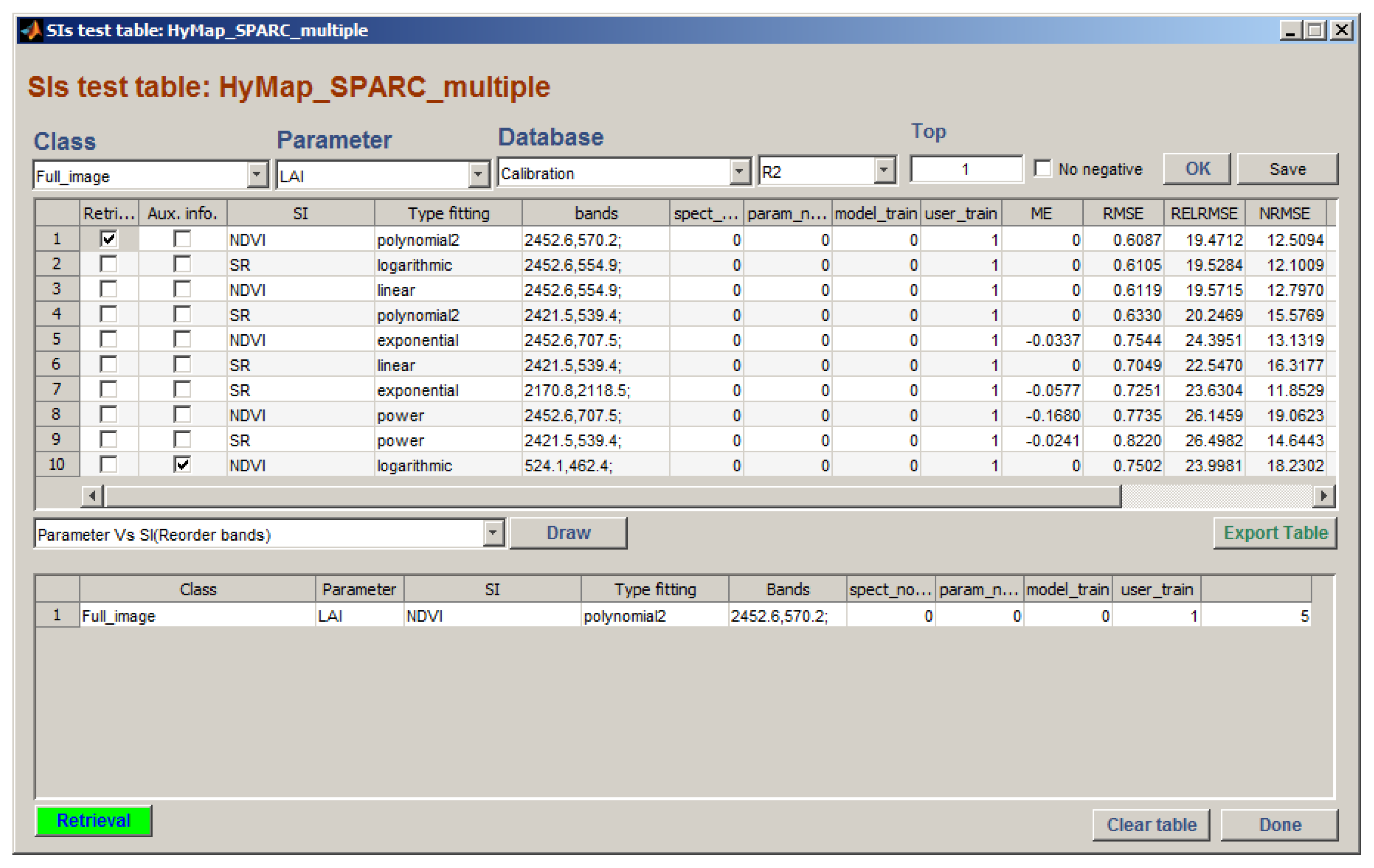
2.4. Calibration/Validation Assessment

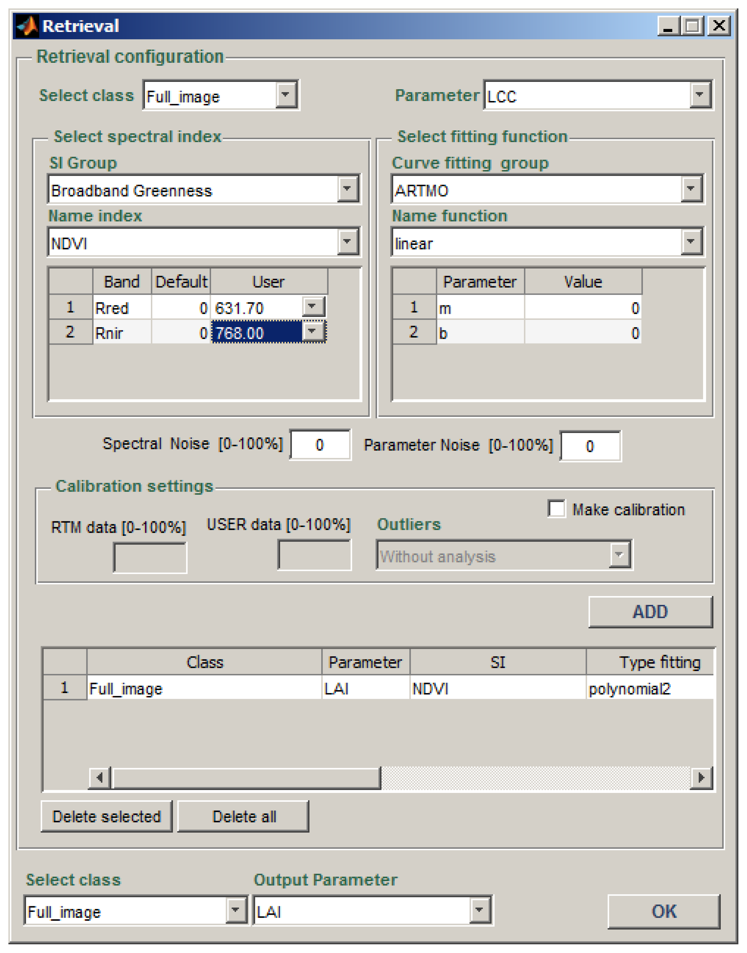
When input data were correctly imported in ARTMO, cal/val data partitioning has been defined and the configuration of SI settings has been successful, the SI models can be assessed with respect to retrieval accuracy. This analysis starts by assigning a name to a new test dataset in the “Test SI” menu. The specified retrieval strategies for the SI formulations and spectral band ranges are then analyzed one-by-one. The assessment results are saved by default in the MySQL database. This way, a large number of SIs can be systematically assessed, and results can be stored and queried. An overview table is then assembled, in which assessment results with the highest accuracy scores are dynamically presented; e.g., per land cover type, per parameter, and per cal/val dataset (see Figure 5). Assessment is then performed. First, for each SI, all spectral band combinations are correlated against the calibration dataset (results not shown). Second, each SI model obtained according to the chosen fitting function is applied to the estimation of a targeted biophysical parameter. When the dataset has previously been partitioned into a calibration and validation set, the assessments are generated twice; one time for the calibration dataset and a second time for the validation dataset. The obtained SI models are evaluated with multiple goodness-of-fit measures like the r², the root mean squared error (RMSE), the normalized RMSE (NRMSE (%) = RMSE/(value range of parameters as measured in the field) × 100), the mean absolute error (MAE) and the mean error (ME). All measures indicate the degree of association between predicted and estimated values of the same parameter and give thus an indication of prediction efficiency. Richter et al. [42] recommended the combined set of r², RMSE and NRMSE, amongst others, for comprehensively quantification the performance of vegetation biophysical models. For a single SI model selected, an option has been foreseen in the GUI, to generate a scatterplot of the retrievals in function of the cal/val measurements (see Section 4). Additionally, by selecting a statical measure, a 2D correlation matrix can be assembled along 2 spectral dimensions, enabling the visualization of the most sensitive 2-band combinations. Finally, for each retrievable biophysical parameter, based on its accuracy assessment, an SI model can be selected and visualized. The selected SI model, e.g., the best performing one, can be accessed through the “Retrieval” GUI window and may be applied using an EO image for spatially distributed biophysical parameter mapping.

2.5. Retrieval

The “Retrieval” window enables to run an assessed SI model, or to directly configure an SI model and apply it to map retrieved parameter values (Figure 6). The latter option can be useful when dealing with a pre-defined SI model (e.g., when an SI is applied as published in the EO literature) or when cal/val datasets are not available. Hence, the user can select a specific land cover type (if available), a biophysical parameter to be retrieved, an SI group and an SI, a regression function and the regression function parameters. The user will be able to select one or multiple remote sensing images for which the evaluated SI model will be applied. Biophysical parameter maps are subsequently stored on disc in ENVI format.

3. Assessment and Mapping Applications

As outlined in the previous section, the SI assessment toolbox is applied to assess the performance of multiple SI regression models with respect to estimation accuracy. Data used are presented first, followed by the experimental setup. Goodness-of-fit results for calibrated SI models are presented and finally the retrieved spatial maps of biophysical parameters are shown. Presented results as generated by the toolbox illustrate its utility, and in principle any type of index can be evaluated. This work ends with recommendations towards a new generation of spectral indices.

3.1. Used Data

A field dataset, encompassing different crop types, growing phases, canopy geometries and soil conditions has been acquired during the SPectra bARrax Campaign (SPARC). The SPARC-2003 campaign took place from 12 to 14 July in Barrax, La Mancha, Spain (coordinates 30°3′N, 28°6′W, 700 m altitude A.S.L.). Biophysical parameters have been measured within a total of 108 Elementary Sampling Units (ESUs) for different crop types (garlic, alfalfa, onion, sunflower, corn, potato, sugar beet, vineyard and wheat). An ESU refers to a plot, which is sized compatible with pixel dimensions of about 20 m × 20 m. Leaf Chlorophyll Content (LCC) was determined by measuring about 50 leaf samples in each ESU with a calibrated CCM-200 Chlorophyll Content Meter [43]. Green LAI was derived from canopy measurements made with a LiCor LAI-2000 digital analyzer. Each ESU was assigned a LAI value, obtained as a statistical mean of 24 measurements (8 data readings × 3 replica) with standard errors ranging from 5% to 10% [44]. Strictly speaking, due to the assumption of a random distribution of foliage, the impact of clumping has been assessed only partially using the LiCor and the corresponding software. Hence, effective LAI is given as an output parameter. For all ESUs, LAI ranges from 0.4 to 6.2 (m² single sided leaf surface)/(m² ground surface) while LCC ranges from 2 to 51 (μg chlorophyll)/(cm² leaf area). Regarding LCC, it should be noted that its measurements were unevenly distributed, with many data points between 40–50 and around 20, but no data points between 25 and 35 μg/cm². No additional bare soil samples were added.

During the campaign, airborne hyperspectral HyMap flightlines have been acquired for the study site, during the month of July 2003. HyMap flew with a configuration of 125 contiguous spectral bands, spectrally positioned between 430 and 2490 nm. Spectral bandwidth varied between 11 and 21 nm. The pixel size during overpass was 5 m. The flight-lines were corrected for radiometric and atmospheric effects according to the procedures of [45,46]. Finally, a calibration dataset was prepared, which refers to the centre pixel of each ESU and corresponding LCC and LAI values.

3.2. Experimental Setup

The SI assessment toolbox has been applied to evaluate the retrieval accuracies for different SI formulations, band settings, and fitting functions using the SPARC calibration dataset. Only the two-band results for the most common SI formulations are illustrated, being SR and ND SI combination types. Correlating the possible HyMap two-band SIs according to these combination types and by using five fitting functions (linear, exponential, power, logarithmic and polynomial of the second degree), the SI assessment toolbox did finally automatically assess 155,000 (125 × 124 × 5 × 2) SI regression functions for each biophysical parameter. This typical assessment run did not take longer than a few minutes on a 32 bit PC (Windows 7 Intel(R) Core(TM) 2 Quad CPU, 2.4 GHz, 3.00 GB RAM processor).

4. Results & Discussion

4.1. Optimized SI’s

For each SI type,

Table 1. Goodness-of-fit measures (RMSE, NRMSE, r²) for the best calibrated SI models per SI type and their corresponding used bands and fitting function for LAI and LCC retrieval. In this table, the SI types are sorted according to a decreasing r². B₁: spectral band 1, B₂: spectral band 2.

Index type	Fitting function	B1 (nm)	B2 (nm)	SI model	abs. RMSE	NRMSE (%)	r2
LAI:
ND	polynomial	570	2453	LAI = −1.366ND2 + 6.154ND + 1.976	0.61	12.51	0.83
SR	logarithmic	555	2453	LAI = 2.291 log(SR) + 1.924	0.61	12.10	0.83
ND	linear	555	2453	LAI = 5.023ND + 1.922	0.61	12.80	0.83
SR	polynomial	539	2421	LAI = −0.621SR2 + 3.754SR −0.760	0.63	15.58	0.82
SR	linear	539	2421	LAI = 1.751SR + 0.504	0.70	16.32	0.77
SR	exponential	2118	2171	LAI = 0.000238e8.783SR	0.72	11.85	0.77
ND	exponential	707	2453	LAI = 0.712e2.721ND	0.75	13.13	0.77
ND	power	707	2453	LAI = 4.670ND0.548	0.77	19.06	0.77
SR	power	539	2421	LAI = 1.951SR1.112	0.82	14.64	0.76
ND	logarithmic	462	524	LAI = 3.888 log(ND) + 6.947	0.85	18.23	0.74
LCC:
ND	polynomial	692	1686	LCC = −227.499ND2 + 281.410ND − 36.924	4.21	7.75	0.93
SR	polynomial	692	1661	LCC = −8.114ND2 + 60.997ND − 61.553	4.30	7.64	0.92
ND	logarithmic	692	1340	LCC = 43.578 log(ND) + 63.272	4.70	10.18	0.91
SR	linear	692	1340	LCC = 7.455SR + 4.707	4.70	20.24	0.91
ND	linear	692	1340	LCC = 90.290ND − 14.808	4.21	10.75	0.90
SR	logarithmic	692	1200	LCC = 26.447 log(ND) − 2.990	5.53	11.54	0.87
SR	exponential	692	1215	LCC = 91.164e−4.235SR	6.00	11.25	0.87
ND	power	632	1698	LCC = 127.581ND2.119	28.06	365.5	0.87
ND	exponential	632	1257	LCC = 2.110e3.827ND	6.64	12.80	0.84
SR	power	707	723	LCC = 7.281SR2.938	8.28	13.19	0.76

provides goodness-of-fit statistics (RMSE, NRMSE and r²) for the best performing calibrated SI models together with its wavelength specifications and regression equation, ranked according to r². The following observations can be made:

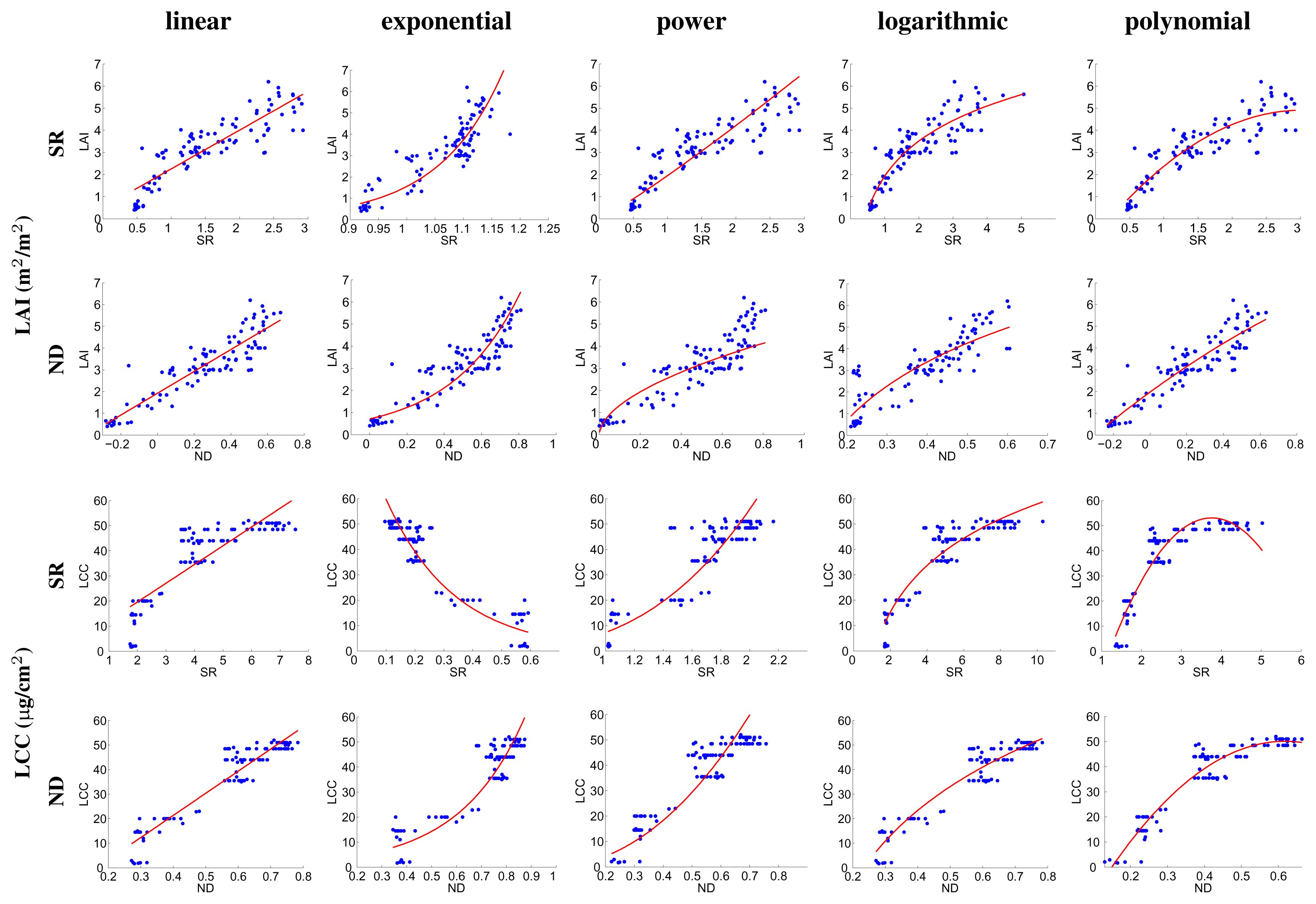
• With regard to SI formulations, no strong evidence has been found that the widely used ND formulation outperforms the less popular SR formulation. Though, it is also recognized that the main argument for using ND types of indices is not the improved correlation performance in comparison to SRs, but rather the (at least to some extent) improved comparability of different observation times/dates and the possible reduction of effects of varying illumination intensity (shades, etc.), due to the inherent normalization of the value range [47]. The ND outperformed the SR for both LAI and LCC only when a second order polynomial is applied as a fitting function. However, when a conventional linear regression is applied, ND performs similar (LCC) or superior (LAI) to SR;
• While the polynomial fit outperforms to some extent the linear regression fitting scenario, the linear fit model is nonetheless accurate as well. For instance, the best linear regression fit outperforms the more sophisticated exponential and power curve fitting approaches significantly for both, LAI and LCC;
• For the majority of the most accurate regression functions, about the same spectral band locations were assessed as being optimal for biophysical parameter retrieval. For LAI, two-band formulations are optimal at 570, 555, 539 and 707 nm with the second band at 2453 or 2421 nm. For LCC two-band locations at 692 nm and 632 nm with the second band at 1661–1698 nm or 1200–1340 nm performed best.

It is noteworthy that, for a majority of the most accurate SI models sensitive with respect to LCC, the wavelength location of 692 nm is ranked as the best performing one. This is consistent with earlier studies (e.g., [24,48]), demonstrating that the spectral interval around 700 nm is less prone to saturation than the location at 660 nm (which coincides with the location of the chlorophyll pigment’s main absorption peak). Therefore, the far-red at 692 nm ensures a good sensitivity when detecting moderate and high LCC values.

Although Table 1 suggests that the optimal fitting functions lead to similar performances in terms of r², a closer look may be necessary to assess their performance in mapping applications. Figure 7 provides scatterplots of the best performing SI models; the distinct behavior of each fitting function can be observed. For instance, exponential and power function fits can lead to spurious parameter value retrievals at high SI values (or at low SI values in case of the SR-LCC combination). The most accurate fitting function, i.e., the second order polynomial, is probably the most difficult one to interpret. This is illustrated for the LCC-SR case where the peak of the polynomial fit goes through the LCC data clumping between 40 and 50 μg/cm². It implies that a SR above 4 leads to a lower LCC estimate. This type of erratic fits indicates that polynomial fitting—despite the high r² and low RMSE—should not be recommended for biophysical parameter retrieval.

Although dating from the times where the campaigns mostly were limited to the silicon-based CCD detector range (400–1000 nm), the saturation effect is often reported and is considered as one of the major critical points when using a Red-NIR formulation (e.g., NDVI) for LAI retrieval [49,50]. A noteworthy observation is that here LAI hardly shows saturation for a linear model fit. Results presented suggest that the use of a band in the SWIR range (2453 nm) causes the saturation effect to be close to negligible. Hence, such a linear regression should be preferred above using the NIR, because saturation violates the assumptions of regression residuals around zero in order for the results to be valid [51]. In addition, [52,53] found that vegetation indices (VIs) based on bands in the SWIR range tend to be almost linearly related to LAI without showing saturation even at high LAI values (LAI = 6). However, it should also be remarked that wavelengths at the end of HyMap sensor’ SWIR range (i.e., beyond 2400 nm) face a relatively low signal-to-noise ratio (SNR), i.e., below 400 [54]. Results in this region may therefore be biased by noise influence.

4.2. Correlation Matrices

To fully take account of the prediction efficiency of the spectral domain, Figure 8 illustrates all two-band SR and ND combinations according to r² correlation between measured and estimated values for the LAI and LCC biophysical parameters for different fitting functions. The correlation matrices for B₁ (430–2490 nm) versus B₂ (430–2490 nm) clearly distinguish the following spectral regions: the visible region (450–700 nm), the red-edge region (700–750 nm), the NIR region (750–1340 nm), the shortwave SWIR region (1470–1800 nm) and the longwave SWIR region (1970–2453 nm). Based on the 2D correlation plots in Figure 8, the spectral regions leading to the most accurate indices to retrieve LAI and LCC can be unequivocally identified. Based on Table 1, the following observations can be made for two-band (B₁, B₂) SIs:

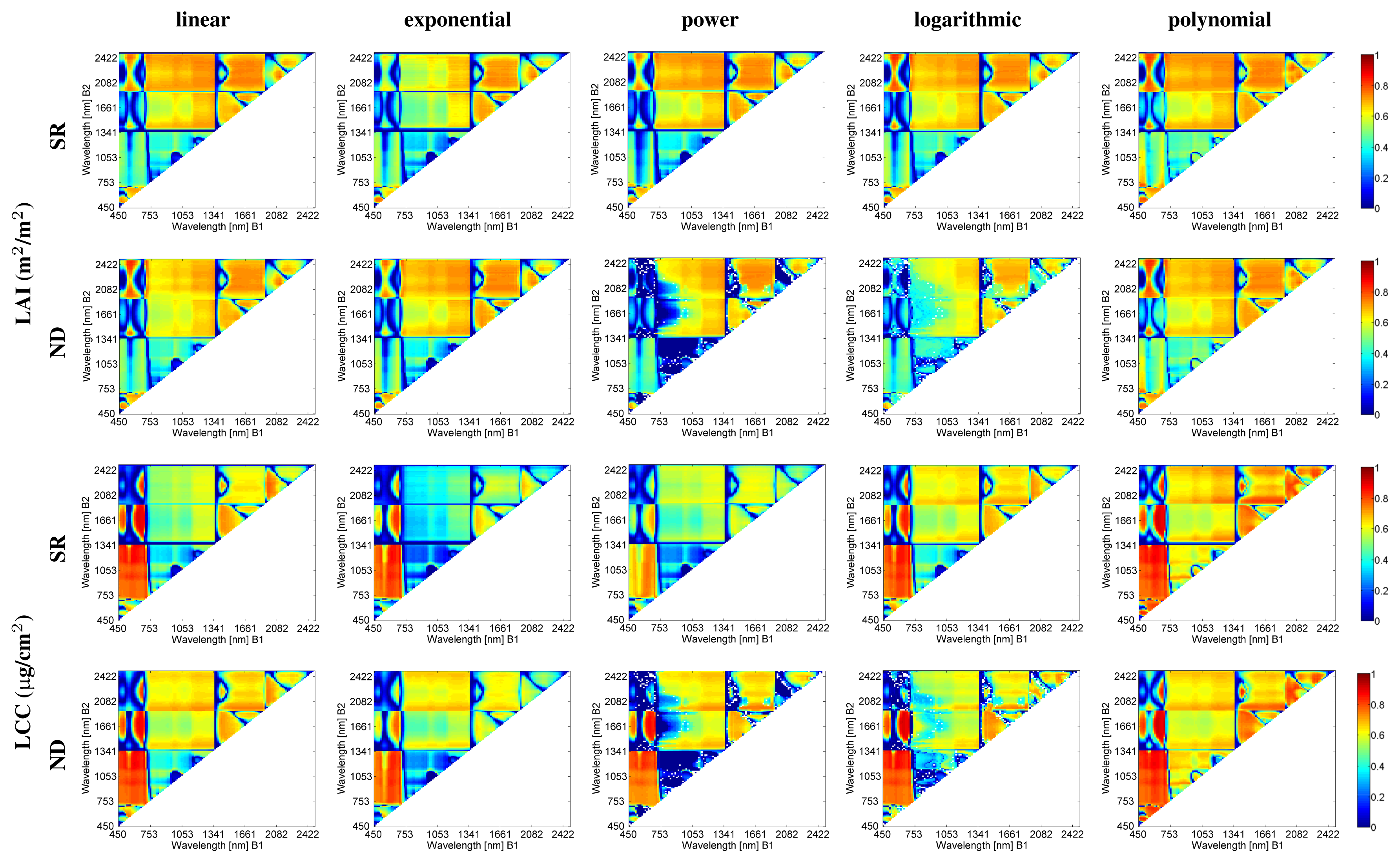
• SR and ND formulations lead to the same spectral regions exhibiting strong correlations between the LAI/LCC biophysical parameters and the two-band SIs. For instance, similar patterns for B₂ in the visible spectral region can be observed. However, the ND power and logarithmic functions fail as good fitting functions for several band combinations. Specifically, they provide lower regression accuracies for B₁ (740–1000 nm) and B₂ (1400–2200 nm);
• Similar patterns with strong and low correlation values are found across the different curve fitting functions assessed. This suggests that the major impact on retrieval accuracy in EO does not originate from the chosen curve fitting but rather from the spectral dimension. Though, local differences do occur. These local differences are particularly pronounced along exponential, power and logarithmic fittings, characterized by quite low correlation values. Hence, the following sections are limited to the discussion of linear and polynomial curve fits;
• For LAI, Figure 8 shows that the most important spectral region for retrieval is the 539–707 nm region for the B₁band, whereas B₂ is located in the longwave SWIR. Notice the hourglass shape in the SWIR region. A second spectral region of maximal r² for B1 is the 1300–1500 nm region as well as the region at 1400–1800 nm. These regions are spectrally quite broad, meaning that the spectral indices do not require very narrow and hence precisely positioned spectral bands, at least for the samples that were used in this study for the generation of the empirical relationships;
• For LCC, Figure 8 shows that the most important spectral region for retrieval is the visible region, particularly the red region until the red edge. B₂ is spectrally located in the shortwave SWIR. Another sensitive zone, having the same B₁ (around 692 nm) as in the first case, has its second band B₂ in the NIR range as well as in the longwave SWIR. Note that these spectral areas are covered by broad spectral bands.

Considering only the linear and polynomial fitting functions, it is of interest that the two-band combinations that were found to be optimal for LAI retrieval in the longwave SWIR region for B₂ (notice the hourglass shape with B₁ centered around the green; 550–570 nm) oppositely lead to suboptimal LCC retrievals. This spectral region can hence be applied for LAI retrieval without being influenced by sensitivity to LCC. For LCC, on the other hand, the most optimal B₁ spectral regions are the NIR and shortwave SWIR in combination with red bands for B₂. Hence, a clearcut distinction can be observed for the sensitive spectrally important regions for the retrieval of LAI versus LCC. Retrieval confusion between LAI and LCC is thereby avoided. The correlation matrices additionally suggest that the SWIR region is preferred above the NIR region, ensuring independent retrievals for LAI and LCC. For instance, the conventional NDVI spectral bands (i.e., B₁ = 680 nm, B₂ = 800 nm) do not appear as most optimal ones for LAI nor LCC retrieval.

4.3. LAI & LCC Mapping

The final step presented in this paper involves LAI and LCC mapping. ARTMO’s SI assessment toolbox helps the user to select a SI model (e.g., the most accurate one) and to apply it using EO imagery. The impact of the SI model type on biophysical parameter mapping thus can be compared. For this purpose, it was opted to map LAI and LCC based on the available HyMap data for the most accurate SI model only, being a linear, logarithmic and polynomial of the second order function. Exponential and power functions have not been considered for mapping, not only because of their considerably less performing calibration results, but also because these functions do not consistently lead to maps conform with ground observations. To allow for a comprehensive visual comparison between retrievals and ground samples, LAI maps are color scaled for values between 0 and 6 m²/m². Identically, LCC maps are color scaled for values between 0 and 60 μg/cm². These maps, as presented in Figure 9, lead to the following observations:

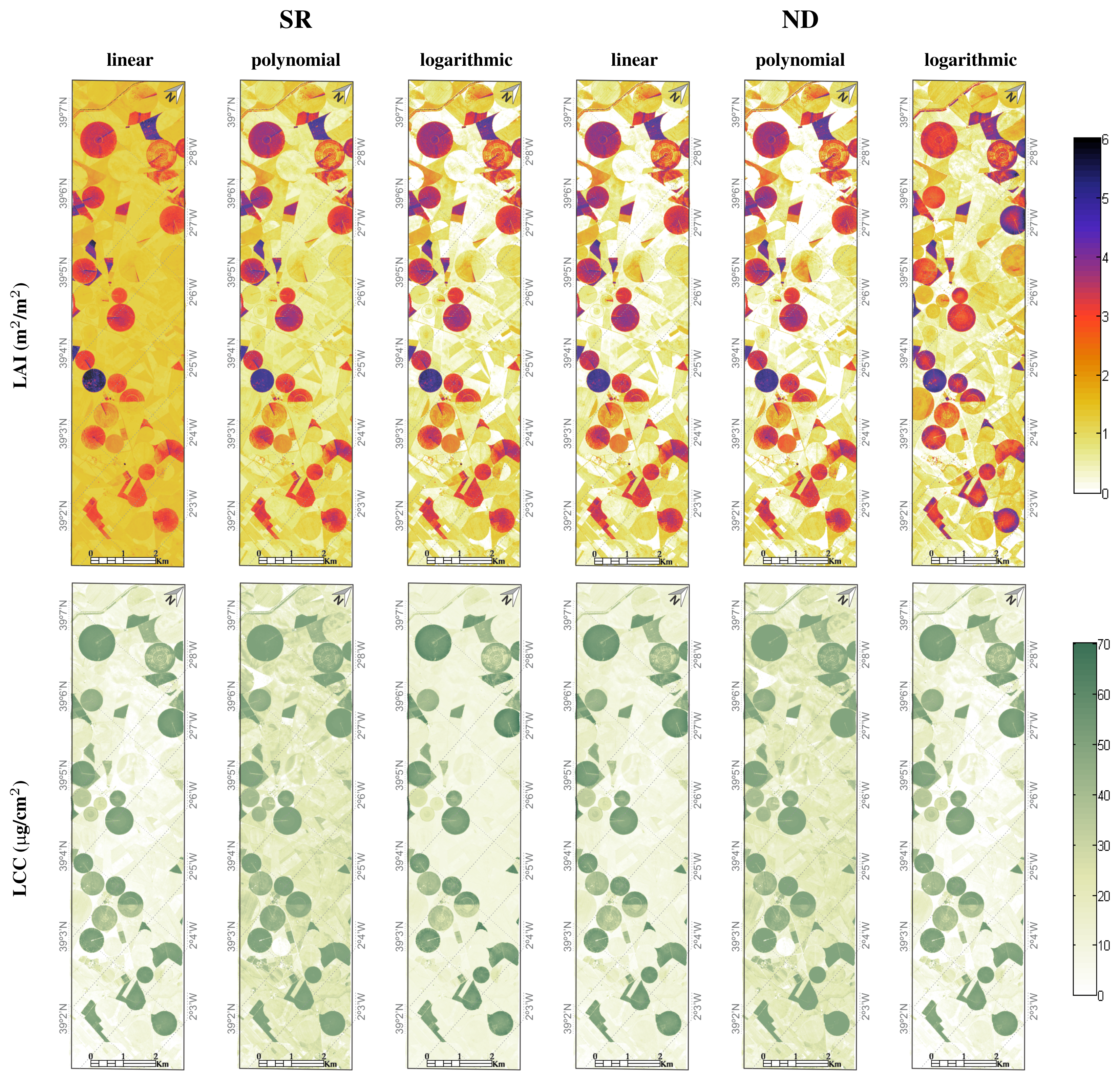
• For LAI, both, the ND polynomial and ND linear regression models, lead to the same calibration result (RMSE = 0.61; r² = 0.83) and accordingly to very similar LAI maps. This example provides confidence that a linear regression is able to deliver adequate LAI maps, when appropriate spectral bands are selected; i.e., green spectral region (B₁: 539–570 nm) in combination with the longwave SWIR (B₂: 1970–2453 nm). Rapid saturation of the LAI in function of the SI is thereby avoided. The map shows areas with a high LAI quite clearly (irrigated circular fields). Areas with a low LAI—senescent crops to bare soil surfaces—elicit a zero value LAI (white color code);
• Conversely, when using SR for LAI mapping, prominent spatial differences appeared for the linear versus polynomial and logarithmic regression models. Particularly, a linear regression exhibits problematic behavior, since LAI variations for senescent regions significantly deviate from the other LAI mapping results. Due to variable soil contribution, a simple linear fit will never be able to capture the variability for near zero LAI values compatible with high LAI values. A logarithmic fitting function seems to lead to more consistent LAI maps. Nevertheless, although the ND type yields considerably poorer calibration results, both maps yield similar LAI patterns. The spatial similarity of the three best performing fitting functions (SR, logarithmic, ND linear and ND polynomial) provide confidence in the realism of the maps produced;
• With regard to LCC mapping, the spatial similarity between the SR and ND polynomial fits and the degree of detail is remarkable. However, interpretation becomes difficult for areas earlier identified as having low LAI values in the LAI map and showing high LCC values in the LCC map. One interpretation may be that the nature of a polynomial of second degree fit leads to retrievals of high LCC values at near-zero SI values. Another problem might be related to the difficulty of upscaling. For the areas where the canopy is very sparse, i.e., the LAI is low, it becomes harder to perceive the chlorophyll pigments in the leaves with a moderate spatial resolution of 1–4 m, even if the chlorophyll concentration in the small leaves is relatively high;
• Logarithmic ND fits, along with linear SR and ND fits, elicit the most realistic LCC patterns; with spatial patterns conform to those of the best LAI maps.

Quite remarkably, the different fitting functions lead to considerable local spatial variation. This can be problematic, since it suggests that the prediction efficiency results on their own may be insufficient as an assessment criterion for the quality of the mapping results. An important aspect to be taken into consideration is that an independent validation dataset likewise gives limited assessment information of the complete map due to a typically low spatial cover within a remote sensing image. Hence, the question arises, which maps—as a whole—are quantitatively most trustworthy? This rather enigmatic problem area reveals one of the main weaknesses of SI based biophysical parameter mapping e.g., the absence of an uncertainty metric on a per-pixel basis. Uncertainty estimates on a pixelwise basis provide an indication of retrieval accuracy and are nowadays a prerequisite in processing chains. In part, this is why more sophisticated regression algorithms have been developed, which do provide associated uncertainty estimates, e.g., in the emerging field of Bayesian approaches such as Gaussian processes regression [33]. Nevertheless, if any generalization can be deduced from the maps presented, for LAI the ND polynomial (second degree) fit leads to the most consistent map, while for LCC it is rather the ND logarithmic fit that leads to the most consistent map when comparing to earlier generated maps [41]. Conversely, the dissimilarity across the SR-developed maps suggests that SR is a less successful formulation for biophysical parameter mapping. The maps provided here suggest that a normalized difference (ND) formulation can therefore be considered as a more preferable strategy for biophysical parameters mapping.

4.4. Towards a New Generation of Spectral Indices

With ARTMO’s SI assessment toolbox extensive and systematic SI performance assessments can be conducted, including band combinations, formulations and fitting functions. Its semi-automatic nature enables the reduction of time and resources for analysis and interpretation. By analyzing all bands against each other in a correlation matrix, ARTMO helps identifying redundant bands and overcoming the Hughes’ phenomenon or “curse of dimensionality” [32]. The case presented in this paper, shows the analysis of all possible 2-band combinations according to SR and ND formulation by using four types of curve fittings on hypespectral data. While the relevance of the visible and red edge spectral regions is widely known for LCC and LAI estimation, and has since long been documented for vegetation mapping applications [19,30,55–57], the sensitivity in the SWIR is particularly remarkable. Especially for LAI retrieval, but also for that of LCC, the SWIR region was found to be an optimal region for biophysical parameter mapping, each time in combination with the visible region; for LAI, green (B₁) with longwave SWIR (B₂), for LCC red (B₁) with shortwave SWIR (B₂). The green-SWIR indices do not show an apparent saturation in the value range considered for LAI, so that the transfer function can be defined with a linear regression model. Similar improvements have been reported by previous studies [52,53,58–61]. In the SWIR, leaf reflectance is mainly controlled by water absorption, although leaf biochemical components such as proteins, cellulose, and lignin also contribute to a lesser extent to leaf absorption (e.g., [62]). In view of mapping a whole agroecosystem, the spatio-structural variables governing reflectance at canopy scale are at least as important. For the Barrax test site, the main drivers of LAI and LCC spatial variation are irrigation regimes, leading to high LCC parcels (when irrigated and due to high water absorption) in contrast to non-irrigated low LCC parcels, which are senescent during summertime. Canopy structural differences depending on the crop type are a source of variation related to both biophysical parameters as well [63]. The SWIR is sensitive to intrinsic variations in soil optical properties as well as variations induced by soil moisture changes [64] and variations in complex and dissimilar growth stages and growing conditions [65,66]. Moreover, the SWIR spectral region has the advantage of being sensitive to vegetation, while being less influenced by atmospheric aerosols [60]. As remarked by the latter author, this avoids the increase in parameter retrieval uncertainty associated with the atmospheric correction of remotely sensed reflectances required to compensate for aerosol scattering impacts on top-of-atmosphere reflectances, typically playing a role in the visible part of the solar spectrum.

When comparing literature findings, where similar correlation matrices are presented, it is remarkable that identical band combinations are rarely reported for studies based on the use of narrowband (hyperspectral) imaging [31,60,61]. This leads us to suggest that established SI models are often case specific and thus are likely to perform sub-optimal for local hyperspectral mapping applications. Quite often, the traditional Red-NIR combination is applied. At the same time, suboptimal SI formulations or regression function selections also lead to less optimal biophysical parameter retrievals. An in-depth analysis is therefore not a luxury. The SI assessment toolbox in ARTMO, as described in this paper, offers a systematic, semi-automatic streamlined and complete procedure for the selection as well an assessment of the most accurate and sensitive SI formulations for biophysical parameter retrieval based on hyperspectral image datasets. The SI model(s) selected can hence confidently be applied for the mapping of biophysical parameters retrieved from hyperspectral imagery.

Finally, it is foreseen that the ARTMO SI assessment toolbox will serve future sensitivity studies. This may lead to a generation of new SIs based on the following recommendations:

• Development and evaluation of generic SIs by using RTMs including viewing and solar geometry. ARTMO includes turbid (e.g., SAIL) as well as explicit 3D RTMs (e.g., FLIGHT). Evidently, the validity of the most optimal models will be assessed using in situ validation data;
• New types of index formulations will be developed and tested across the full optical spectrum. Only SR and ND indices have been assessed here. Yet, alternative mathematical formulations are to be tested as well, e.g., the formulations used for soil adjusted vegetation index (SAVI), enhanced vegetation index (EVI), weighted difference vegetation index (WDVI) or more complex ones;
• Although in this paper only two-band formulations have been assessed, the SI toolbox offers the option for a systematic analysis of a full optical spectrum of band combinations with SI formulations of up to ten different bands in the range of 400 to 2500 nm. Since there is no reason to believe that two-band indices lead to the most successful SI models, this multiple band approach may lead to the development of more accurate and sensitive spectral indices.

Regardless of the above-mentioned research objectives, essentially, the SI assessment toolbox provides all necessary tools for quality assurance and quality control (QA/QC), and for a rapid and comprehensive biophysical parameter mapping. The toolbox is intuitive and can assist significantly in precision farming and landscape ecology monitoring applications, thereby allowing to optimize SIs, even per land cover type.

5. Conclusions

A newly developed Spectral Indices (SI) assessment toolbox in the ARTMO modeling environment enables the analysis and assessment of the accuracy of an indefinite number of SI models. Basically, the toolbox offers a systematic but still empirical approach for the assessment of all possible band combinations with SI formulations of up to 10 different bands. Datatsets may originate from simulations, e.g., as generated by the optical radiative transfer models in ARTMO, or from field campaigns. Several options have been included in the SI assessment approach, amongst which: (1) The addition of noise and the possibility to select fitting functions (e.g., linear, exponential, power or polynomial functions); (2) the SI toolbox virtually allows for any type of spectral index model to be formulated and evaluated using up to ten spectral bands; and (3) the possibility to assess and apply SIs per land cover class.

Using HyMap data calibrated with field measured data, the predictive power of generic narrowband spectral indices in the 430–2490 nm range to quantify LAI and LCC has been assessed. For LAI retrieval, the B₁ in the green (B₁: 539, 555, 570 nm) combined with longwave SWIR (e.g., B₂: 2421, 2453 nm) has been evaluated as the most accurate approach (RMSE: 0.61; r²: 0.83). For LCC retrieval, the B₁ in the far-red (692 nm) combined with the B₂ NIR (e.g., 1340 nm) or shortwave SWIR (e.g., 1661, 1686 nm) has been evaluated as the most accurate approach (RMSE: 4.21–4.70, r²: 0.91–0.93). In either case, the identification of the SWIR, instead of the conventional NIR, as an important spectral region reinforces our suggestion that the ARTMO SI assessment toolbox significantly facilitates the development of new and especially better performing spectral indices for biophysical parameter mapping applications.

References

1. Moulin, S.; Bondeau, A.; Delécolle, R. Combining agricultural crop models and satellite observations: From field to regional scales. Int. J. Remote Sens 1998, 19, 1021–1036. [Google Scholar]
2. Báez-González, A.; Chen, P.Y.; Tiscareño López, M.; Srinivasan, R. Using satellite and field data with crop growth modeling to monitor and estimate corn yield in Mexico. Crop Sci 2002, 42, 1943–1949. [Google Scholar]
3. Dorigo, W.A.; Zurita-Milla, R.; de Wit, A.J.W.; Brazile, J.; Singh, R.; Schaepman, M.E. A review on reflective remote sensing and data assimilation techniques for enhanced agroecosystem modeling. Int. J. Appl. Earth Obs. Geoinf 2007, 9, 165–193. [Google Scholar]
4. Drusch, M.; del Bello, U.; Carlier, S.; Colin, O.; Fernandez, V.; Gascon, F.; Hoersch, B.; Isola, C.; Laberinti, P.; Martimort, P.; et al. Sentinel-2: ESA’s optical high-resolution mission for GMES operational services. Remote Sens. Environ 2012, 120, 25–36. [Google Scholar]
5. Donlon, C.; Berruti, B.; Buongiorno, A.; Ferreira, M.H.; Femenias, P.; Frerick, J.; Goryl, P.; Klein, U.; Laur, H.; Mavrocordatos, C.; et al. The Global Monitoring for Environment and Security (GMES) Sentinel-3 mission. Remote Sens. Environ 2012, 120, 37–57. [Google Scholar]
6. Stuffler, T.; Kaufmann, C.; Hofer, S.; Forster, K.; Schreier, G.; Mueller, A.; Eckardt, A.; Bach, H.; Penne, B.; Benz, U.; et al. The EnMAP hyperspectral imager—An advanced optical payload for future applications in Earth observation programmes. Acta Astronaut 2007, 61, 115–120. [Google Scholar]
7. Roberts, D.; Quattrochi, D.; Hulley, G.; Hook, S.; Green, R. Synergies between VSWIR and TIR data for the urban environment: An evaluation of the potential for the Hyperspectral Infrared Imager (HyspIRI) decadal survey mission. Remote Sens. Environ 2012, 117, 83–101. [Google Scholar]
8. Labate, D.; Ceccherini, M.; Cisbani, A.; de Cosmo, V.; Galeazzi, C.; Giunti, L.; Melozzi, M.; Pieraccini, S.; Stagi, M. The PRISMA payload optomechanical design, a high performance instrument for a new hyperspectral mission. Acta Astronaut 2009, 65, 1429–1436. [Google Scholar]
9. Myneni, R.; Maggion, S.; Iaquinta, J.; Privette, J.; Gobron, N.; Pinty, B.; Kimes, D.; Verstraete, M.; Williams, D. Optical remote sensing of vegetation: Modeling, caveats, and algorithms. Remote Sens. Environ 1995, 51, 169–188. [Google Scholar]
10. Gobron, N.; Pinty, B.; Verstraete, M.; Widlowski, J.L. Advanced vegetation indices optimized for up-coming sensors: Design, performance, and applications. IEEE Trans. Geosci. Remote Sens 2000, 38, 2489–2505. [Google Scholar]
11. Houborg, R.; Boegh, E. Mapping leaf chlorophyll and leaf area index using inverse and forward canopy reflectance modeling and SPOT reflectance data. Remote Sens. Environ 2008, 112, 186–202. [Google Scholar]
12. Rivera, J.; Verrelst, J.; Leonenko, G.; Moreno, J. Multiple cost functions and regularization options for improved retrieval of leaf chlorophyll content and LAI through inversion of the PROSAIL model. Remote Sens 2013, 5, 3280–3304. [Google Scholar]
13. Verrelst, J.; Rivera, J.; Leonenko, G.; Alonso, L.; Moreno, J. Optimizing LUT-based RTMinversion for semiautomatic mapping of crop biophysical parameters from Sentinel-2 and -3 data: Role of cost functions. IEEE Trans. Geosci. Remote Sens 2013, 52, 257–269. [Google Scholar]
14. Chen, J.; Cihlar, J. Retrieving leaf area index of boreal conifer forests using Landsat TM images. Remote Sens. Environ 1996, 55, 153–162. [Google Scholar]
15. Myneni, R. Estimation of global leaf area index and absorbed PAR using radiative transfer models. IEEE Trans. Geosci. Remote Sens 1997, 35, 1380–1393. [Google Scholar]
16. Combal, B.; Baret, F.; Weiss, M.; Trubuil, A.; Macé, D.; Pragnère, A.; Myneni, R.; Knyazikhin, Y.; Wang, L. Retrieval of canopy biophysical variables from bidirectional reflectance using prior information to solve the ill-posed inverse problem. Remote Sens. Environ 2003, 84, 1–15. [Google Scholar]
17. Broge, N.; Mortensen, J. Deriving green crop area index and canopy chlorophyll density of winter wheat from spectral reflectance data. Remote Sens. Environ 2002, 81, 45–57. [Google Scholar]
18. Haboudane, D.; Miller, J.; Pattey, E.; Zarco-Tejada, P.; Strachan, I. Hyperspectral vegetation indices and novel algorithms for predicting green LAI of crop canopies: Modeling and validation in the context of precision agriculture. Remote Sens. Environ 2004, 90, 337–352. [Google Scholar]
19. Thenkabail, P.; Smith, R.; de Pauw, E. Evaluation of narrowband and broadband vegetation indices for determining optimal hyperspectral wavebands for agricultural crop characterization. Photogramm. Eng. Remote Sens 2002, 68, 607–621. [Google Scholar]
20. Ustin, S.; Roberts, D.; Gamon, J.; Asner, G.; Green, R. Using imaging spectroscopy to study ecosystem processes and properties. BioScience 2004, 54, 523–534. [Google Scholar]
21. Hatfield, J.; Gitelson, A.; Schepers, J.; Walthall, C. Application of spectral remote sensing for agronomic decisions. Agron. J 2008, 100, S117–S131. [Google Scholar]
22. Baret, F.; Guyot, G. Potentials and limits of vegetation indices for LAI and APAR assessment. Remote Sens. Environ 1991, 35, 161–173. [Google Scholar]
23. Verrelst, J.; Schaepman, M.; Koetz, B.; Kneubuhler, M. Angular sensitivity analysis of vegetation indices derived from CHRIS/PROBA data. Remote Sens. Environ 2008, 112, 2341–2353. [Google Scholar]
24. Verrelst, J.; Schaepman, M.E.; Malenovský, Z.; Clevers, J.G.P.W. Effects of woody elements on simulated canopy reflectance: Implications for forest chlorophyll content retrieval. Remote Sens. Environ 2010, 114, 647–656. [Google Scholar] [Green Version]
25. Ceccato, P.; Flasse, S.; Grégoire, J.M. Designing a spectral index to estimate vegetation water content from remote sensing data: Part 1: Theoretical approach. Remote Sens. Environ 2002, 82, 188–197. [Google Scholar]
26. Zarco-Tejada, P.; Miller, J.; Noland, T.; Mohammed, G.; Sampson, P. Scaling-up and model inversion methods with narrowband optical indices for chlorophyll content estimation in closed forest canopies with hyperspectral data. IEEE Trans. Geosci. Remote Sens 2001, 39, 1491–1507. [Google Scholar]
27. Le Maire, G.; François, C.; Dufrêne, E. Towards universal broad leaf chlorophyll indices using PROSPECT simulated database and hyperspectral reflectance measurements. Remote Sens. Environ 2004, 89, 1–28. [Google Scholar]
28. Zarco-Tejada, P.J.; Berjón, A.; López-Lozano, R.; Miller, J.R.; Martín, P.; Cachorro, V.; Gonzalez, M.R.; de Frutos, A. Assessing vineyard condition with hyperspectral indices: Leaf and canopy reflectance simulation in a row-structured discontinuous canopy. Remote Sens. Environ 2005, 99, 271–287. [Google Scholar]
29. Le Maire, G.; François, C.; Soudani, K.; Berveiller, D.; Pontailler, J.Y.; Bréda, N.; Genet, H.; Davi, H.; Dufrêne, E. Calibration and validation of hyperspectral indices for the estimation of broadleaved forest leaf chlorophyll content, leaf mass per area, leaf area index and leaf canopy biomass. Remote Sens. Environ 2008, 112, 3846–3864. [Google Scholar]
30. Delegido, J.; Verrelst, J.; Alonso, L.; Moreno, J. Evaluation of Sentinel-2 red-edge bands for empirical estimation of green LAI and chlorophyll content. Sensors 2011, 11, 7063–7081. [Google Scholar]
31. Mariotto, I.; Thenkabail, P.; Huete, A.; Slonecker, E.; Platonov, A. Hyperspectral versus multispectral crop-productivity modeling and type discrimination for the HyspIRI mission. Remote Sens. Environ 2013, 139, 291–305. [Google Scholar]
32. Thenkabail, P.; Lyon, G.; Huete, A. Advances in Hyperspectral Remote Sensing of Vegetation and Agricultural Croplands. In Hyperspectral Remote Sensing of Vegetation; CRC Press: New York, NY, USA, 2011; pp. 3–29. [Google Scholar]
33. Verrelst, J.; Alonso, L.; Camps-Valls, G.; Delegido, J.; Moreno, J. Retrieval of vegetation biophysical parameters using Gaussian process techniques. IEEE Trans. Geosci. Remote Sens 2012, 50, 1832–1843. [Google Scholar]
34. Feret, J.B.; François, C.; Asner, G.P.; Gitelson, A.A.; Martin, R.E.; Bidel, L.P.R.; Ustin, S.L.; le Maire, G.; Jacquemoud, S. PROSPECT-4 and 5: Advances in the leaf optical properties model separating photosynthetic pigments. Remote Sens. Environ 2008, 112, 3030–3043. [Google Scholar]
35. Stuckens, J.; Verstraeten, W.; Delalieux, S.; Swennen, R.; Coppin, P. A dorsiventral leaf radiative transfer model: Development, validation and improved model inversion techniques. Remote Sens. Environ 2009, 113, 2560–2573. [Google Scholar]
36. Verhoef, W.; Bach, H. Coupled soil-leaf-canopy and atmosphere radiative transfer modeling to simulate hyperspectral multi-angular surface reflectance and TOA radiance data. Remote Sens. Environ 2007, 109, 166–182. [Google Scholar]
37. North, P. Three-dimensional forest light interaction model using a Monte Carlo method. IEEE Trans. Geosci. Remote Sens 1996, 34, 946–956. [Google Scholar]
38. Widlowski, J.L.; Pinty, B.; Lopatka, M.; Atzberger, C.; Buzica, D.; Chelle, M.; Disney, M.; Gastellu-Etchegorry, J.P.; Gerboles, M.; Gobron, N.; et al. The fourth radiation transfer model intercomparison (RAMI-IV): Proficiency testing of canopy reflectance models with ISO-13528. J. Geophys. Res. D Atmos 2013, 118, 6869–6890. [Google Scholar]
39. ARTMO. Available online: http://ipl.uv.es/artmo/ (accessed on 22 May 2014).
40. Verrelst, J.; Romijn, E.; Kooistra, L. Mapping vegetation density in a heterogeneous river floodplain ecosystem using pointable CHRIS/PROBA data. Remote Sens 2012, 4, 2866–2889. [Google Scholar]
41. Rivera Caicedo, J.; Verrelst, J.; Alonso, L.; Moreno, J.; Camps-Valls, G. Toward a semiautomatic machine learning retrieval of biophysical parameters. IEEE J. Sel. Top. Appl. Earth Obs. Remote Sens 2014, 7, 1249–1259. [Google Scholar]
42. Richter, K.; Atzberger, C.; Hank, T.; Mauser, W. Derivation of biophysical variables from earth observation data: Validation and statistical measures. J. Appl. Remote Sens 2012, 6. [Google Scholar] [CrossRef]
43. Gandía, S.; Fernández, G.; Garcia, J.C.; Moreno, J. Retrieval of Vegetation Biophysical Variables from CHRIS/PROBA Data in the SPARC Campaign. Proceedings of the 2nd CHRIS/PROBAWorkshop, Frascati, Italy, 28–30 April 2004.
44. Fernández, G.; Moreno, J.; Gandía, S.; Martínez, B.; Vuolo, F.; Morales, F. Statistical Variability of Field Measurements of Biophysical Parameters in SPARC-2003 and SPARC-2004 Campaigns. Proceedings of the ESA WPP-250—SPARC Final Workshop, Enschede, the Netherlands, 4–5 July 2005.
45. Alonso, L.; Moreno, J. Advances and Limitations in a Parametric Geometric Correction of CHRIS/PROBA Data. Proceedings of the 3rd CHRIS/Proba Workshop, Frascati, Italy, 21–23 March 2005.
46. Guanter, L.; Estellés, V.; Moreno, J. Spectral calibration and atmospheric correction of ultra-fine spectral and spatial resolution remote sensing data. Application to CASI-1500 data. Remote Sens. Environ 2007, 109, 54–65. [Google Scholar]
47. Rouse, J.; Haas, R.; Schell, J.; Deering, D.; Harlan, J. Monitoring the Vernal Advancement of Retrogradation of Natural Vegetation; Remote Sensing Center, Texas A&M University: College Station, TX, USA, 1974. [Google Scholar]
48. Gitelson, A.; Gritz, Y.; Merzlyak, M. Relationships between leaf chlorophyll content and spectral reflectance and algorithms for non-destructive chlorophyll assessment in higher plant leaves. J. Plant Physiol 2003, 160, 271–282. [Google Scholar]
49. Stenberg, P.; Rautiainen, M.; Manninen, T.; Voipio, P.; Smolander, H. Reduced simple ratio better than NDVI for estimating LAI in Finnish pine and spruce stands. Silva Fenn 2004, 38, 3–14. [Google Scholar]
50. Verstraete, M.; Pinty, B. Designing optimal spectral indexes for remote sensing applications. IEEE Trans. Geosci. Remote Sens 1996, 34, 1254–1265. [Google Scholar]
51. Draper, N.; Smith, H. Applied Regression Analysis, 3rd ed; Wiley Series in Probability and Statistics; Wiley: New York, NY, USA, 1998. [Google Scholar]
52. Darvishzadeh, R.; Atzberger, C.; Skidmore, A.; Abkar, A. Leaf Area Index derivation from hyperspectral vegetation indicesand the red edge position. Int. J. Remote Sens 2009, 30, 6199–6218. [Google Scholar]
53. Schlerf, M.; Atzberger, C.; Hill, J. Remote sensing of forest biophysical variables using HyMap imaging spectrometer data. Remote Sens. Environ 2005, 95, 177–194. [Google Scholar]
54. Cocks, T.; Jenssen, R.; Stewart, A.; Wilson, I.; Shields, T. The HyMap Airborne Hyperspectral Sensor: The System, Calibration and Performance. Proceedings of the 1st EARSeL Workshop on Imaging Spectroscopy, Zurich, Switzerland, 6–8 October 1998; pp. 37–42.
55. Filella, I.; Penuelas, J. The red edge position and shape as indicators of plant chlorophyll content, biomass and hydric status. Int. J. Remote Sens 1994, 15, 1459–1470. [Google Scholar]
56. Clevers, J.; Gitelson, A. Remote estimation of crop and grass chlorophyll and nitrogen content using red-edge bands on Sentinel-2 and -3. Int. J. Appl.Earth Obs. Geoinf 2013, 23, 344–351. [Google Scholar]
57. Delegido, J.; Verrelst, J.; Meza, C.; Rivera, J.; Alonso, L.; Moreno, J. A red-edge spectral index for remote sensing estimation of green LAI over agroecosystems. Eur. J. Agron 2013, 46, 42–52. [Google Scholar]
58. Brown, L.; Chen, J.; Leblanc, S.; Cihlar, J. A shortwave infrared modification to the simple ratio for LAI retrieval in boreal forests: An image and model analysis. Remote Sens. Environ 2000, 71, 16–25. [Google Scholar]
59. Lee, K.S.; Cohen, W.; Kennedy, R.; Maiersperger, T.; Gower, S. Hyperspectral versus multispectral data for estimating leaf area index in four different biomes. Remote Sens. Environ 2004, 91, 508–520. [Google Scholar]
60. Gonsamo, A. Normalized sensitivity measures for leaf area index estimation using three-band spectral vegetation indices. Int. J. Remote Sens 2011, 32, 2069–2080. [Google Scholar]
61. Heiskanen, J.; Rautiainen, M.; Stenberg, P.; Mõttus, M.; Vesanto, V.H. Sensitivity of narrowband vegetation indices to boreal forest LAI, reflectance seasonality and species composition. ISPRS J. Photogramm. Remote Sens 2013, 78, 1–14. [Google Scholar]
62. Curran, P. Remote sensing of foliar chemistry. Remote Sens. Environ 1989, 30, 271–278. [Google Scholar]
63. Verrelst, J.; Muñoz, J.; Alonso, L.; Delegido, J.; Rivera, J.; Camps-Valls, G.; Moreno, J. Machine learning regression algorithms for biophysical parameter retrieval: Opportunities for Sentinel-2 and -3. Remote Sens. Environ 2012, 118, 127–139. [Google Scholar]
64. Lobell, D.; Asner, G. Moisture effects on soil reflectance. Soil Sci. Soc. Am. J 2002, 66, 722–727. [Google Scholar]
65. Thenkabail, P.; Smith, R.; de Pauw, E. Hyperspectral vegetation indices and their relationships with agricultural crop characteristics. Remote Sens. Environ 2000, 71, 158–182. [Google Scholar]
66. Thenkabail, P.; Enclona, E.; Ashton, M.; van der Meer, B. Accuracy assessments of hyperspectral waveband performance for vegetation analysis applications. Remote Sens. Environ 2004, 91, 354–376. [Google Scholar]
Figure 1. Screenshot of ARTMO’s main window and schematic overview of its drop-down menu.
Remotesensing 06 04927f1
Figure 2. Screenshot of the ARTMO v3 “Spectral Indices assessment toolbox” and schematic overview of its drop-down menu.
Remotesensing 06 04927f2
Figure 3. GUI section used to add a new SI formulation.
Remotesensing 06 04927f3
Figure 4. SI settings window.
Remotesensing 06 04927f4
Figure 5. SI’s calibration/validation assessment table.
Remotesensing 06 04927f5
Figure 6. SI’s Retrieval window.
Remotesensing 06 04927f6
Figure 7. Fitting functions (red lines) depicting the regression of LAI (m2/m2) and LCC (μg/cm2) in function of SR and ND formulations as they could be derived from the calibration dataset using optimized band combinations.
Remotesensing 06 04927f7
Figure 8. 2D r2 correlation matrices calculated from measured vs. estimated values for the calibration results of the LAI (m2/m2) and LCC (μg/cm2) retrievals according to SR and ND formulations and for different fitting functions. The color bars on the right of this figure give the values of the plotted r2 in the different graphs.
Remotesensing 06 04927f8
Figure 9. LAI (m2/m2) and LCC (μg/cm2) maps based on SR and ND formulations and linear, polynomial and logarithmic fitting functions. The imagery originates from a HyMap flight line over the Barrax agricultural area in Spain. The color bars at the right side of this figure give the values of the LAI and LCC mapped variables.
Remotesensing 06 04927f9