Phytoplankton Biomass Dynamics in the Strait of Malacca within the Period of the SeaWiFS Full Mission: Seasonal Cycles, Interannual Variations and Decadal-Scale Trends

Abstract

Seasonal cycles, interannual variations and decadal trends of Sea-viewing Wide Field-of-view Sensor (SeaWiFS)-retrieved chlorophyll-a concentration (Chl-a) in the Strait of Malacca (SM) were investigated with reconstructed, cloud-free SeaWiFS Chl-a during the period of the SeaWiFS full mission (September 1997 to December 2010). Pixel-based non-parametric correlations of SeaWiFS Chl-a on environmental variables were used to identify the probable causes of the observed spatio-temporal variations of SeaWiFS Chl-a in northern, middle and southern regions of the SM. Chl-a was high (low) during the northeast (southwest) monsoon. The principal causes of the seasonality were wind-driven vertical mixing in the northern region and wind-driven coastal upwelling and possibly river discharges in the middle region. Among the three regions, the southern region showed the largest interannual variations of Chl-a. These variations were associated with the El Niño/Southern Oscillation (ENSO) and river runoff. Interannual variations of Chl-a in the middle and northern regions were more responsive to the Indian Ocean Dipole and ENSO, respectively, with atmospheric deposition being the most important driver. The most significant decadal-scale trend of increasing Chl-a was in the southern region; the trend was moderate in the middle region. This increasing trend was probably caused by environmental changes unrelated to the variables investigated in this study.

1. Introduction

The Strait of Malacca (SM), which connects the Andaman Sea and the South China Sea, is one of the most important international waterways and is also one of the world’s highest blood cockle (Anadara granosa) production areas [1]. Commercial fisheries in the SM, including blood cockle production, depend largely on the primary production of phytoplankton [2,3], as fish and cockle feed directly on phytoplankton, which are the base of the marine food web. Phytoplankton also play an important role in marine biogeochemical cycles. Through photosynthesis, marine phytoplankton assimilate inorganic carbon and, thereby, serve as a sink for atmospheric carbon dioxide. Chlorophyll-a concentration (hereafter Chl-a) is commonly used as a metric of phytoplankton biomass for purposes of estimating primary production from satellite observations. All phytoplankton contain Chl-a, or in the case of Prochlorococcus sp., divinyl Chl-a [4]. Chl-a, however, is subject to spatial and temporal variations, and such variations affect phytoplankton-dependent marine carbon dynamics and higher trophic level marine organisms.

The marine environment of the SM is strongly influenced by the Asian monsoon [5,6]. The Asian monsoon is characterized by annual reversing winds: dry southwesterly winds during the southwest monsoon (SWM, May–August) and wet northeasterly winds during the northeast monsoon (NEM, November–February) [5,6]. During the SWM, the water of the northern SM is influenced by the intrusion of Andaman Sea water driven by southwesterly winds [7], whereas during the NEM, the southern SM is influenced by the intrusion of South China Sea water [7,8]. During the wet NEM, the water of the SM is also greatly influenced by river discharges from both the Indonesian side (Sumatra) and the west coast of Peninsular Malaysia [9].

In addition to the seasonal monsoon winds, the geographic position of the SM, which lies between the Indian and Pacific Oceans, makes the marine environment of the SM subject to the influence of large-scale climatic anomalies, such as the Indian Ocean Dipole (IOD) and the El Niño/Southern Oscillation (ENSO). It is well known that, besides changes in precipitation associated with variations of the trade winds to the west and east of the Indonesian archipelago, both positive IOD and El Niño events bring severe drought to Indonesia, and those droughts are very frequently followed by forest wildfires [10,11]. Forest fires can be important sources of macro- and micro-nutrients for phytoplankton growth, as a result of atmospheric deposition of ash and aerosols [12]. In this way, coupled interactions between the atmosphere and ocean may provide a mechanism by which both the IOD and ENSO influence biological production in the SM. In addition to these natural factors, human activities, such as land clearing, mangrove deforestation and the impacts of rapid population and economic growth along the coastal areas of the surrounding countries (Indonesia, Malaysia and Singapore), also contribute to environmental changes in the SM [1].

These anthropogenic and natural perturbations are expected to cause spatial and temporal variations of oceanographic conditions, including Chl-a and, hence, primary production in the SM. In the SM, Chl-a retrieved by the Sea-viewing Wide Field-of-view Sensor (SeaWiFS) shows distinct seasonal variations [6]. Tan et al. [6] have reported high SeaWiFS Chl-a during the NEM, but low Chl-a during the SWM. However, the details of the mechanisms and the predominant drivers underlying the seasonal Chl-a variations are still unclear, because Tan et al. [6] analyzed SeaWiFS data from a short period of time (1997–2003), and they did not carry out statistical/quantitative analyses to identify the most predominant factor(s) underlying the spatial and temporal SeaWiFS Chl-a variations. In addition, Tan et al. [6] noted that although SeaWiFS Chl-a in the region they defined as the northern SM was in good agreement with in situ Chl-a values, SeaWiFS Chl-a in the southern SM region was much higher than in situ Chl-a values. There has been no discussion about these apparent errors in SeaWiFS Chl-a data or about the implications of such errors with respect to studies of seasonal cycles, interannual variations and long-term trends of SeaWiFS Chl-a. Trends of Chl-a during the last decade and the possibility that large-scale climatic anomalies in the Indian and Pacific Oceans will modulate Chl-a interannual variations in the SM have also not been discussed. The goal of this work was therefore to use multisensor satellite estimates of atmospheric and oceanic variables retrieved during the full 13-year SeaWiFS mission (September 1997, to December 2010) to: (1) discern trends during the last decade, as well as spatial and temporal variations on seasonal and interannual time scales of SeaWiFS Chl-a; and (2) identify the mechanisms and predominant factors driving the trend during the last decade, as well as seasonal and interannual variations of observed Chl-a.

2. Methodology

2.1. Multisensor Satellite Data Acquisition

Chl-a and aerosol optical thickness at 865 nm (AOT) derived from monthly SeaWiFS Level-3 (with 9-km spatial resolution) ocean color data during the full 13-year SeaWiFS mission were used in this study and acquired from the NASA Ocean Biology Processing Group (OBPG) [13]. The latest version of SeaWiFS Chl-a (SeaWiFS Reprocessing 2010.0) was used to ensure the best quality of SeaWiFS Chl-a data. The SeaWiFS Chl-a data used here were processed using the standard black pixel assumption atmospheric correction [14] and retrieved by using the NASA standard OC4v4 empirical Chl-a algorithm [15]. We masked all pixels with negative values of remote sensing reflectance at 412 nm. We considered the data from these pixels to be invalid, because of an atmospheric correction failure.

Monthly sea surface temperature (SST from Physical Oceanography Distributed Active Archive Center (PODAAC)) [16] with 4-km spatial resolution retrieved by the Advanced Very High Resolution Radiometer (AVHRR) from September 1997, to December 2009, and by the Moderate Resolution Imaging Spectroradiometer-Aqua (MODIS) [13] from January 2010, to December 2010, were used to generate an SST dataset compatible with the 13-year SeaWiFS data. Other satellite data used in this study were wind speed (WS) and rain rate (RR), which were retrieved by microwave sensors on the QuikScat satellite (from September 1997, to November 2009, acquired from Remote Sensing Systems (REMSS) [17]) and the Tropical Rainfall Measuring Mission (TRMM) satellite Precipitation Radar (from September 1997, to December 2010, acquired from the Asia-Pacific Data-Research Center [18]), respectively. The spatial resolution of both the monthly WS and RR data was 0.25°. Satellite-derived SST, WS and RR images were re-gridded to match the SeaWiFS Chl-a and AOT image dimensions.

2.2. Satellite Data Processing

Sub-setting of ocean color and SST satellite data to the SM study region (Figure 1) was accomplished by using Unix-based SeaWiFS Data Analysis System (SeaDAS) version 6.4; sub-setting of WS and RR data was carried out by using Matrix Laboratory (MATLAB) software. Although Tan et al. [6] divided the SM into northern and southern regions, we divided the SM into northern, middle and southern regions, because the northern and southern regions are very different in terms of: (1) water optical properties (Case-1 water in the northern region and Case-2 water in the southern region); (2) physical oceanography (largely influenced by Andaman Sea water in the northern region and by South China Sea water in the southern region) [7,8]; and (3) bathymetry and topography (the strait is deep and wide toward the north, but shallow and narrow toward the south). We included the middle region, so that it could serve as a transition region between the northern and southern regions and because it is more influenced by freshwater discharge from four rivers of the total of 12 main rivers in Peninsular Malaysia [9].

Because clouds interfere with SeaWiFS optical and thermal sensors, satellite-retrieved Chl-a, AOT and SST datasets include pixels with no data (missing values). Before conducting analyses of spatial and temporal variations, we reconstructed data missing due to cloud cover by using empirical orthogonal function-based data interpolation (DINEOF) to produce cloud-free satellite Chl-a, AOT and SST datasets. DINEOF is a non-parametric EOF-based method for the reconstruction of missing data or blank pixels [19]. DINEOF was applied by first reconstructing time series satellite data into a three-dimensional matrix. The first two dimensions were spatial dimensions (latitude and longitude), and the third dimension was time (number of months). The missing values in each satellite image were set to not-a-number (NaN). A singular value decomposition technique was then applied to reconstruct the NaN pixels while computing the EOFs of the matrix.

To make AVHRR and MODIS SSTs comparable, MODIS SSTs were linearly regressed against AVHRR SSTs at each pixel. Linear regression was conducted separately on a monthly basis within the period when both AVHRR and MODIS SSTs were available (May 2002, to December 2009). For each month, the regression coefficients (slope and intercept) at each pixel were then used to convert MODIS SSTs to values compatible with AVHRR SSTs. Finally, we used AVHRR SSTs from September 1997, to December 2009, and MODIS SSTs from January 2010 to December 2010, to construct 13-year, satellite-derived SST datasets.

We used the meridional (north-south) wind component (V) and zonal (east-west) wind component (U) derived from QuikScat to estimate the wind stress curl and, thereby, to identify the physical processes likely responsible for modulating the Chl-a via upwelling and downwelling. Following Large and Pond [20], surface wind stress vectors were calculated with the following bulk formulas:

$${\tau }_{\text{y}}=\rho \times {\text{C}}_{\text{D}}\times \text{WS}\times \text{V};\hspace{0.17em}\hspace{0.17em}\hspace{0.17em}\hspace{0.17em}\hspace{0.17em}\hspace{0.17em}\hspace{0.17em}{\tau }_{\text{x}}=\rho \times {\text{C}}_{\text{D}}\times \text{WS}\times \text{U}$$

where τ_x, τ_y, ρ and C_D are zonal wind stress (N·m⁻²), meridional wind stress (N·m⁻²), density of surface air (1.2 kg·m⁻³) and a non-dimensional drag coefficient (0.0012), respectively. The values of τ_x and τ_y were then used to calculate the wind stress curl (curl_τ, Pa·m⁻¹) as follows:

$${\text{curl}}_{\tau }=\frac{\partial {\tau }_{\text{y}}}{{\partial }_{\text{x}}}-\frac{\partial {\tau }_{\text{x}}}{{\partial }_{\text{y}}}$$

Pixel-based non-parametric correlations of SeaWiFS Chl-a on the other satellite-retrieved variables were used to derive correlation coefficients (hereafter, referred to as r values, with statistical significance) and to identify relationships. To identify the possible impacts of large-scale climatic anomalies associated with IOD and ENSO on interannual variations of SeaWiFS Chl-a, Chl-a anomalies were compared to the Dipole Mode Index (DMI acquired from Japan Agency for Marine-Earth Science and Technology (JAMSTEC) [21]) and Nino3.4 SST anomalies (Nino3.4 acquired from the NOAA Climate Prediction Center (CPC) [22]). The DMI is an anomalous SST gradient between the western (50–70°E and 10°S to 10°N) and southeastern (90–110°E and 10°S–0°N) equatorial Indian Ocean and is used to identify the phase of an IOD event. The Nino3.4 is an ENSO phase indicator derived by averaging SST anomalies in the region bounded by 5°N to 5°S and 170–120°W.

To assess trends in Chl-a, we used the Chl-a anomaly (hereafter Chl-a_an1), which was derived by removing the seasonal cycle of Chl-a from the Chl-a time series. However, when assessing interannual variations of Chl-a, we derived the Chl-a anomaly differently. We first removed the seasonal cycle of Chl-a from the Chl-a time series and then removed the trend (hereafter Chl-a_an2). This metric of Chl-a interannual variation was therefore not confounded by seasonal cycles and long-term trends. There remained only the signature of interannual variability associated with large-scale climatic anomalies. Relationships between the Chl-a_an2 and the anomalies of other variables were investigated to discern the variables that probably accounted for the Chl-a interannual variations. Anomalies of other satellite-retrieved environmental variables were also derived using the same procedure (i.e., the suffixes, _an1 and suffix _an2, were also used for other variables).

2.3. Monthly Climatology of River Discharge

Information on the monthly discharges of the rivers that empty into the SM within the period of this study was not available. We therefore acquired monthly climatological river discharge (RD) data archived by the Center for Sustainability and the Global Environment (SAGE) [23] for the four main rivers (Selangor, Perak, Klang and Langat) that empty into the SM (Figure 1).

As an initial attempt to identify the importance of RD in driving the Chl-a seasonal cycle in the SM, we compared monthly climatological RD to monthly climatological Chl-a. This comparison of climatological values was meaningful only for discerning seasonal cycles. We could not discern the importance of RD as a cause of interannual variations and trends of Chl-a in this study.

3. Results and Discussion

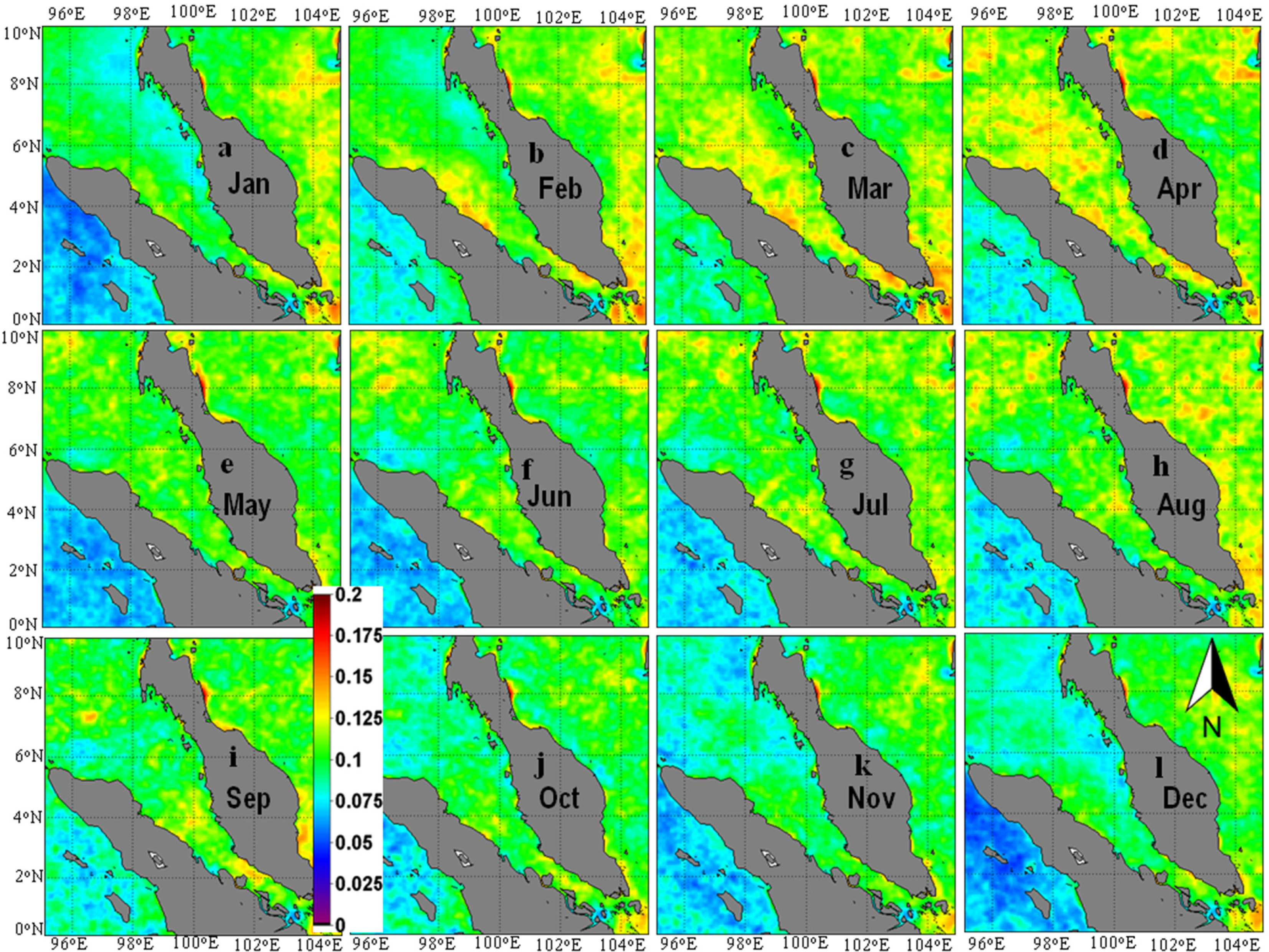
3.1. Seasonal Cycles, Interannual Variations and Decadal-Scale Trends of SeaWiFS Chl-a

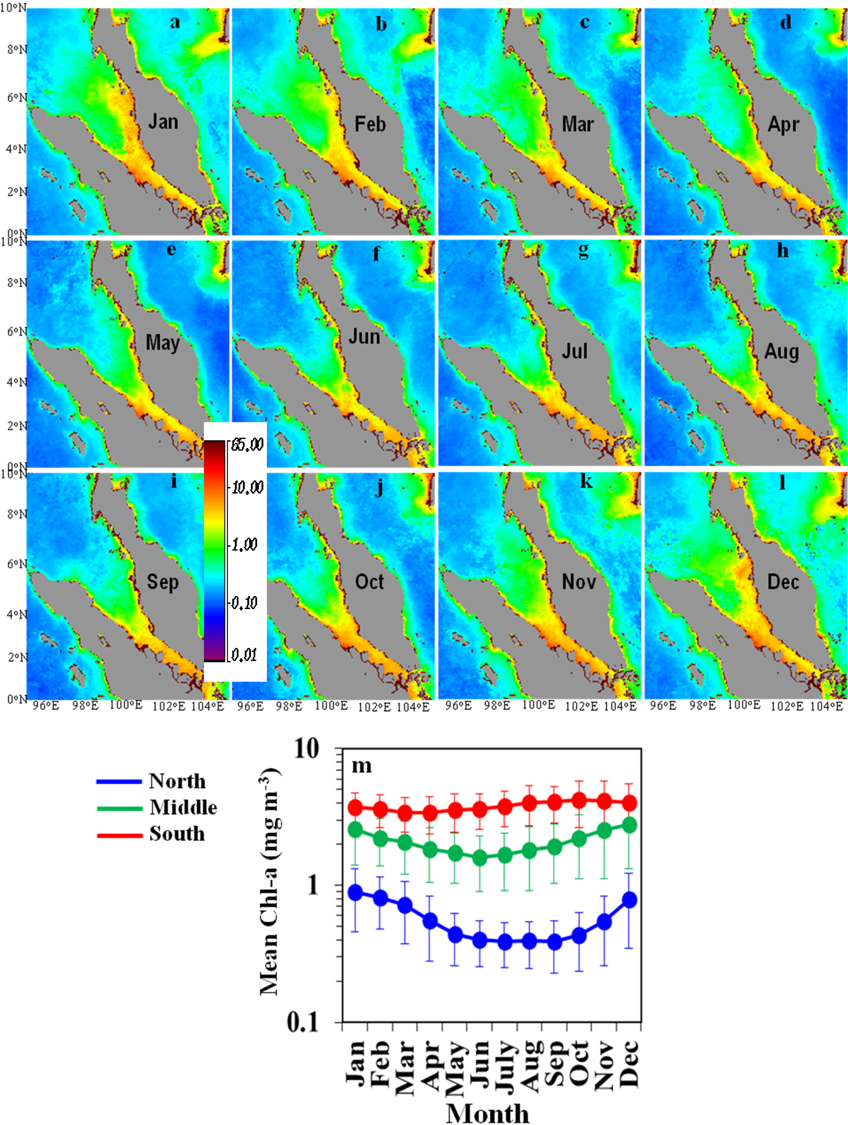
Over the entire region of the SM, a remarkable seasonal cycle of Chl-a was apparent; Chl-a was high during the NEM (Figure 2a,b,k,l) and low during the SWM (Figure 2e–h). A distinct seasonal variation of monthly climatological means of Chl-a was apparent in all three regions of the SM. The time series of SeaWiFS data from 1997 to 2010 revealed a seasonal peak of Chl-a in the southern region during October (Figure 2m), consistent with the results of Tan et al. [6], which were based on a shorter time series of SeaWiFS Chl-a data (1997–2003). The consistency between our results and those of Tan et al. [6] is not surprising, because our southern region was geographically almost identical to Tan et al.’s [6] southern region. Tan et al.’s [6] northern region, however, encompassed both the northern and middle regions defined in this study. Although the Chl-a seasonal cycles were similar in our northern and middle regions, those two regions were remarkably different in terms of monthly climatological means and ranges of variation (quantified in terms of standard deviations) of Chl-a. The peak of the Chl-a bloom during the NEM also occurred earlier in the middle region (in December) than in the northern region (in January). Tan et al. [6] missed this meridional difference in the timing of the peak of the Chl-a bloom during the NEM, because they combined both the northern and middle regions of our study into their single northern region. It is obvious from our study that the highest Chl-a during the NEM tend to occur progressively earlier from the northern to the southern regions.

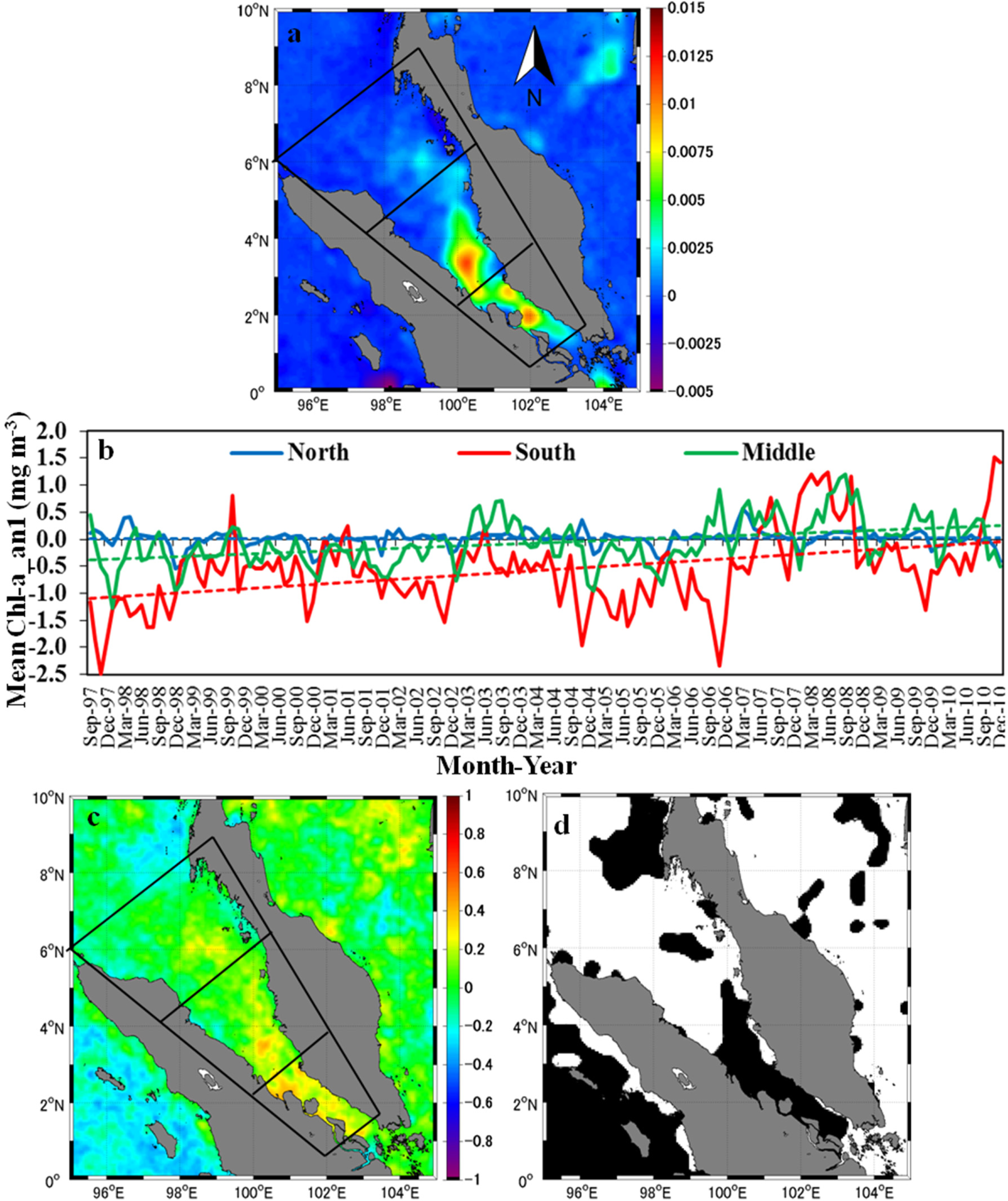
During the SeaWiFS full mission, the Chl-a_an1 (seasonality-removed Chl-a anomaly) tended to increase, both in the middle and southern regions. The rates of increase or slopes were about 0.004 mg·m⁻³·month⁻¹ and 0.007 mg·m⁻³·month⁻¹, respectively, or about 0.05 mg·m⁻³·yr⁻¹ and 0.08 mg·m⁻³·yr⁻¹, respectively (Figure 3a,b). During the last decade of SeaWiFS, the rates of increase of Chl-a in the middle and southern regions were significant, as evidenced by the significant positive correlation (r > 0.4, p < 0.0001) between Chl-a_an1 and time (Figure 3c,d). The trend of increasing Chl-a in the middle region was likely due more to the increasing trend of Chl-a in the southeastern part of the middle region (Figure 3a,c,d), where the rate of change was greater than 0.005 mg·m⁻³·month⁻¹ or 0.06 mg·m⁻³·yr⁻¹. In the northern region of the SM, however, despite a conspicuous Chl-a seasonal cycle, almost no trend of Chl-a was apparent in the last decade of SeaWiFS (Figure 3a,b), as evidenced by the absence of a significant correlation between Chl-a_an1 and time (Figure 3c,d).

A four-month moving average of Chl-a_an2 (seasonality-removed and detrended Chl-a anomaly) revealed that the largest Chl-a interannual variations occurred in the southern region of the SM, whereas the smallest interannual variations occurred in the northern region (Figure 4a). Chl-a interannual variations in the southern region were particularly apparent during the period from September 1997, to May 1998, and from July 2004 to March 2007, when Chl-a tended to be low. The periods from January 1999 to September 2001, from September 2007 to November 2008, and during September 2010, however, were characterized by high Chl-a.

Interannual variations of Chl-a in the southern region were inversely associated with Nino3.4 (Figure 4a), as is also evidenced by the significant negative correlation between Chl-a_an2 and Nino3.4 (r = −0.52, p < 0.01) (

Table 1. Correlation coefficients (r-values) associated with linear regressions of chlorophyll-a concentration anomaly (Chl-a_an2) on DMI (second column), Nino3.4 (third column), aerosol optical thickness anomaly (AOT_an2, fourth column), rain rate anomaly (RR_an2, fifth column), zonal wind anomaly (U_an2, sixth column), meridional wind anomaly (V_an2, seventh column) and wind speed anomaly (WS_an2, eighth column) in the northern, middle and southern regions of the SM. Because there were no wind field observations in the southern region, the r associated with regressions of SeaWiFS Chl-a_an2 on wind field anomalies in the southern region were derived by using wind field anomalies from the middle region of the SM on the assumption that characteristics of the middle region wind field were, to some degree, also representative of the southern region wind field. Associations between Chl-a and sea surface temperature (SST) are not mentioned here, because SST is not the factor that causes temporal variations of Chl-a.

Region	DMI	Nino3.4	AOT_an2	RR_an2	U_an2	V_an2	WS_an2
North	0.18*	0.26**	0.25*	0.18*	−0.21*	−0.06#	−0.01#
Middle	0.31**	0.15#	0.19*	0.20*	−0.14#	0.16#	−0.10#
South	−0.13#	−0.52**	0.05#	0.17*	0.08#+	−0.05#+	0.16#+

^#p> 0.05;

^*p < 0.05;

^**p< 0.01;

⁺wind field data from the middle region of the SM were used.

). This relationship implies that Chl-a in the southern region of the SM tended to be low during El Niño (positive Nino3.4) and high during La Niña (negative Nino3.4) years. In contrast, in the northern region, there was a statistically significant positive correlation (r = 0.26, p < 0.01) between Nino3.4 and Chl-a_an2. There was also a significant positive correlation (r = 0.18, p < 0.05) between Chl-a_an2 and DMI in the northern region, but this correlation was weaker than the positive correlation between Chl-a_an2 and Nino3.4. In the middle region, however, there was no apparent association between Chl-a_an2 and Nino3.4 (Figure 4a, Table 1), but there was a significant positive correlation (r = 0.31, p < 0.01) between Chl-a_an2 and DMI.

3.2. Correlations between SeaWiFS Chl-a and Other Satellite-Retrieved Environmental Variables

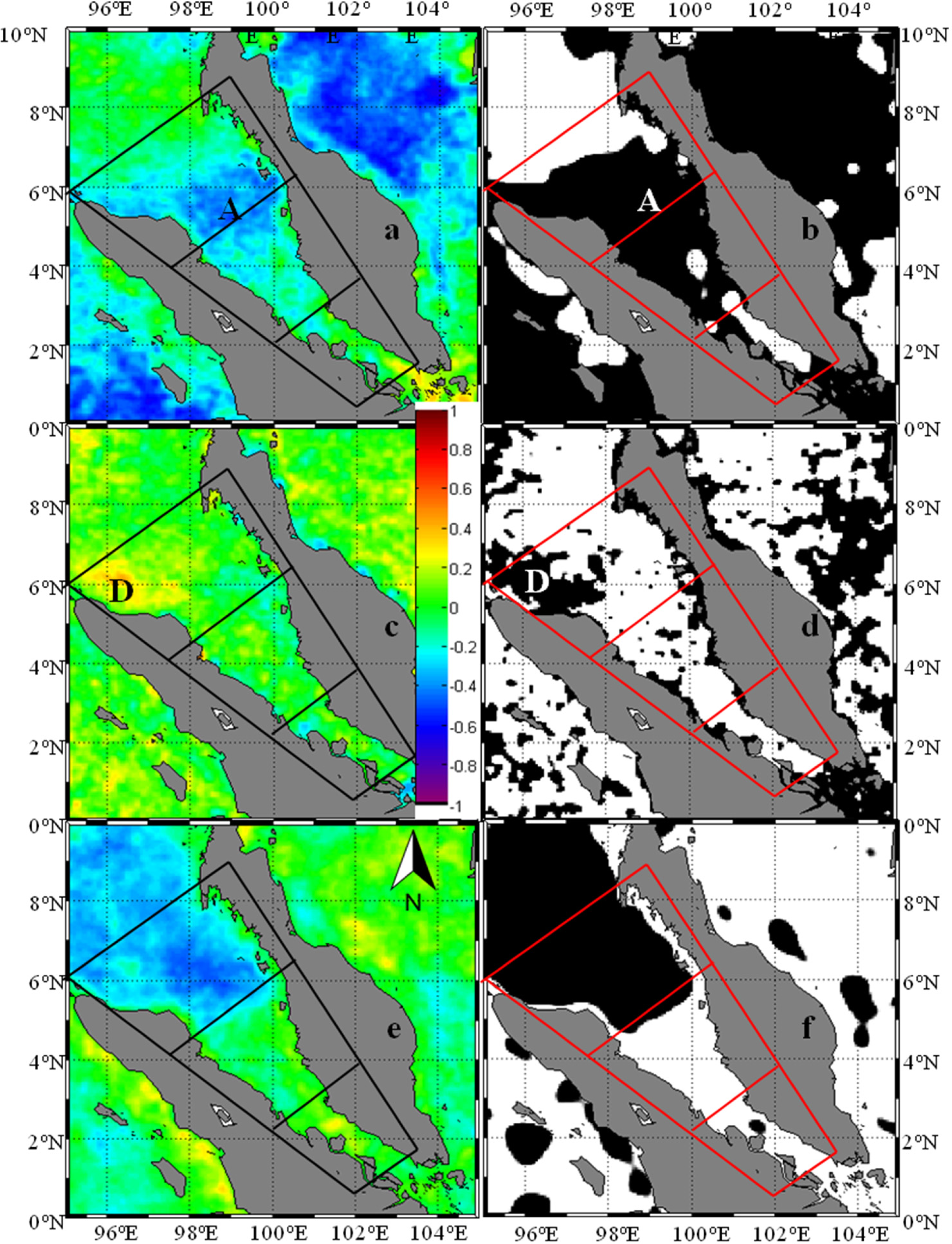
On a seasonal timeframe, we used non-parametric correlation (with no time lag) to investigate pixel-based relationships between Chl-a and other satellite-derived environmental variables, the goal being to discern the factors that were likely responsible for the seasonal and spatial variations of Chl-a in the SM. A statistically significant negative correlation (r < −0.4, p < 0.05) between Chl-a and SST was apparent over a wide area within the northern and middle regions of the SM (Area A in Figure 5a,b). There was almost no significant relationship between Chl-a and AOT, except for an area in the northwestern part of the SM northern region (Area D in Figure 5c,d), where there was a significant positive correlation (r > 0.3, p < 0.05) between Chl-a and AOT. There was a very significant negative correlation (r < −0.4, p < 0.05) between RR and Chl-a in the northern region of the SM (Figure 5e,f). This significant negative correlation extended to the Andaman Sea, whereas in the SM middle and southern regions, there was almost no association between Chl-a and RR.

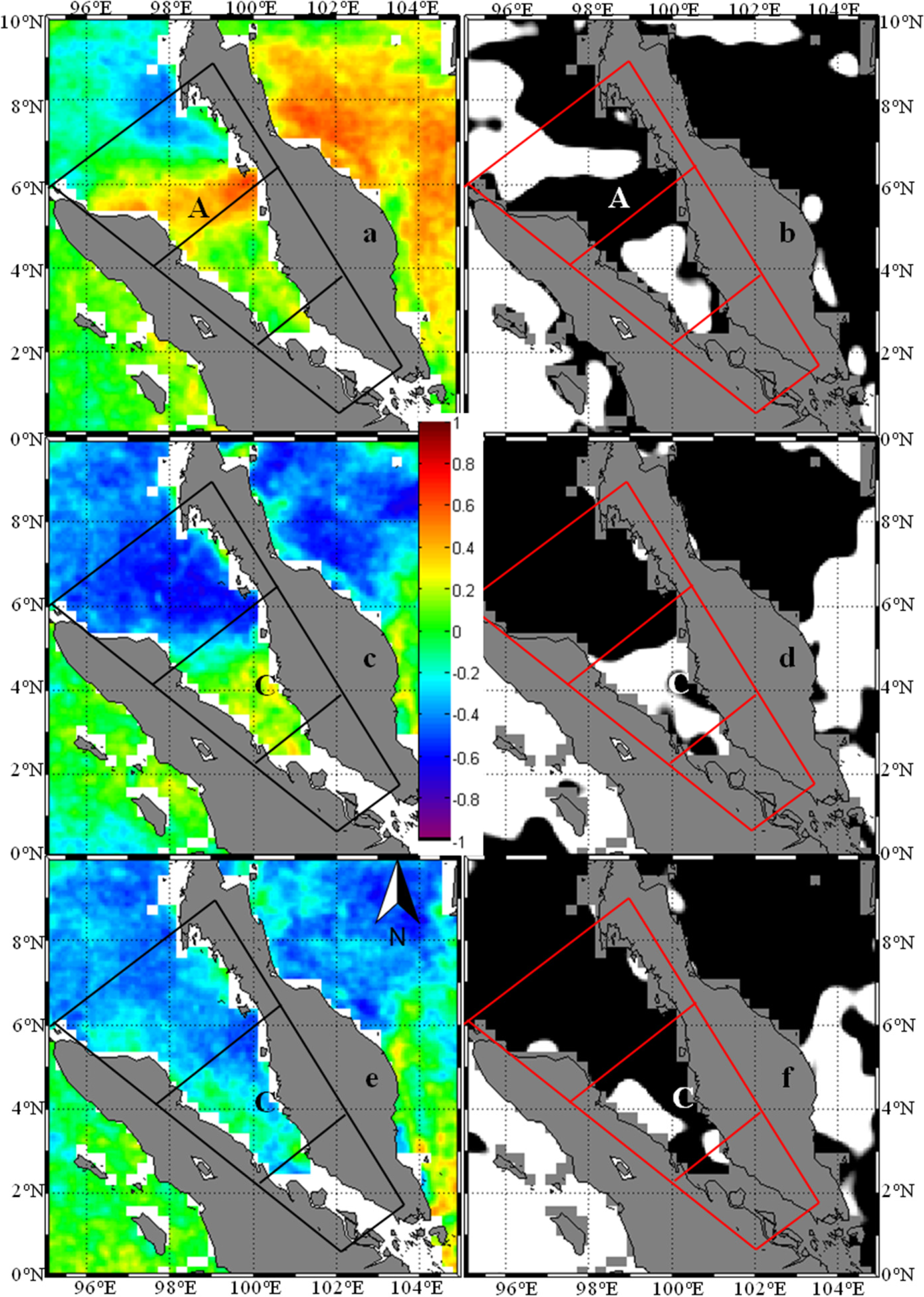
An east-west, belt-like pattern of significant positive correlation (r > 0.5, p < 0.05) between Chl-a and WS was apparent approximately in Area A (Figure 6a,b). There was no significant correlation between Chl-a and WS within a large portion of the middle region of the SM and northern part of the northern region of the SM. There was a significant negative correlation (r < −0.5, p < 0.05) between U and Chl-a in the northern region of the SM (Figure 6c,d). However, a significant positive correlation coefficient (r > 0.3, p < 0.05) was apparent in some pixels near the coastal regions (Area C). Like U, V also showed a significant negative correlation with Chl-a (r < −0.3, p < 0.05) in the northern region of the SM (Figure 6e,f). In the Peninsular Malaysian coastal area of the middle region of the SM (Area C), a significant negative correlation was also observed, but no significant correlation was apparent on the opposite side (the coastal area of Sumatra).

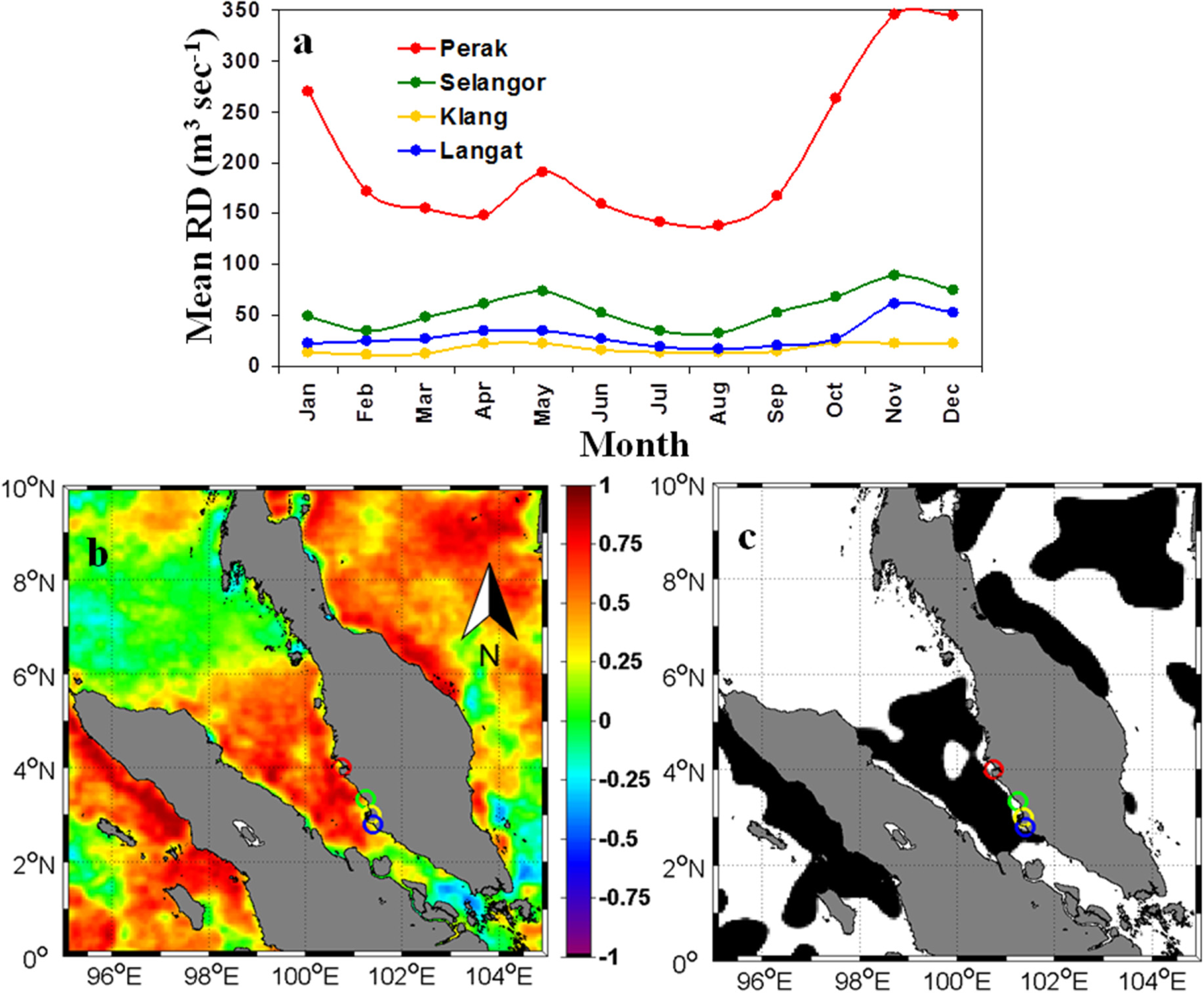
The monthly climatological mean of RD was highest in November, especially in the cases of the Perak, Selangor and Langat Rivers (Figure 7a). The average RR over Peninsular Malaysia was also highest during November (Figure 8k). The fact that the period of second highest RD was April–May is also consistent with the relatively high RR along the western side of Peninsular Malaysia (Figure 8d,e). High RR during the NEM inevitably increases freshwater discharge into the SM, as evidenced by the minimum of surface salinity during the NEM [24]. Besides transporting freshwater, RD also transports nutrients from the land into the SM. A significant positive correlation (r > 0.5, p < 0.05) between monthly climatological Chl-a and monthly climatological RD (average for the four main rivers, Figure 7b,c) in approximately the same area of RD-diluted, low-salinity water [24] may reflect the role of the seasonality of RR in determining seasonal Chl-a variations in the SM through the influx of nutrients from the land.

To identify the probable drivers of interannual variations of Chl-a associated with large-scale climatic anomalies, we computed the correlation between SeaWiFS Chl-a_an2 and other variable anomalies (seasonality-removed and detrended anomalies). Interannual Chl-a variations in the northern region of the SM were significantly correlated with the AOT anomaly (AOT_an2) (r = 0.25, p < 0.05, Table 1), the indication being that AOT was the main driver responsible for the interannual variations of Chl-a associated with both ENSO and IOD events. U seemed to be the second-most important driver of interannual variations of Chl-a, as evidenced by the significant negative correlation (r = −0.21, p < 0.05) between the U anomaly (U_an2) and Chl-a_an2. In the middle region of the SM, RR seemed to be the primary factor responsible for interannual variations of Chl-a associated with the IOD, as evidenced by the significant positive correlation (r = 0.20, p < 0.05) between SeaWiFS Chl-a_an2 and the RR anomaly (RR_an2). The second most important variable was AOT, as evidenced by the significant positive correlation (r = 0.19, p < 0.05) between SeaWiFS Chl-a_an2 and AOT_an2. In the southern region of the SM, RR seemed to be the most important driver of Chl-a interannual variations associated with ENSO events, as evidenced by the significant correlation (r = 0.17, p < 0.05) between SeaWiFS Chl-a_an2 and RR_an2.

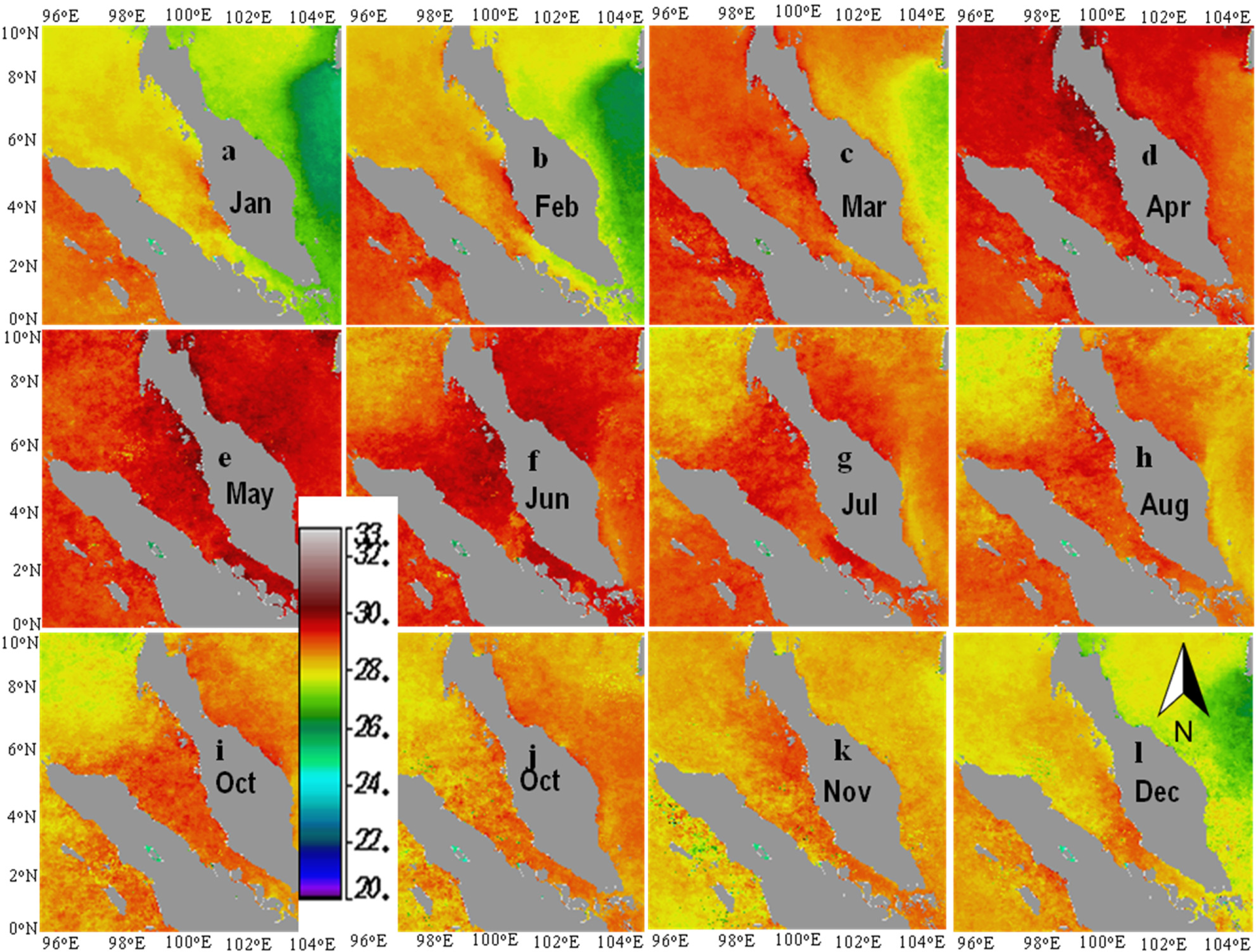
3.3. Factors Responsible for the SeaWiFS Chl-a Seasonal Cycle

The seasonal cycle of Chl-a was apparent both in the northern and middle regions of the SM (Figure 2m), where Chl-a showed a significant negative correlation with SST (Figure 5a,b), a reflection of the seasonal association between high (low) Chl-a and low (high) SST during the NEM (SWM) (Figures 2 and 9). The negative correlation between SST and Chl-a implies that SST was not a factor that drove the Chl-a seasonal cycle. The negative correlation between Chl-a and SST contradicts the basic tenet of temperature-dependent phytoplankton growth [25]. The negative correlation between Chl-a and SST, however, may be indicative of nutrient-limited phytoplankton growth [26], especially considering that SST is consistently higher than 20 °C throughout the year (Figure 9).

The seasonal cycles of Chl-a in the northern and middle regions of the SM must, therefore, be associated with seasonal cycles of nutrient fluxes. Nutrients can be supplied by vertical fluxes (by dry or wet atmospheric deposition and by deep water upwelling/mixing) and from horizontal nutrient fluxes (loading by RD) [27–29]. 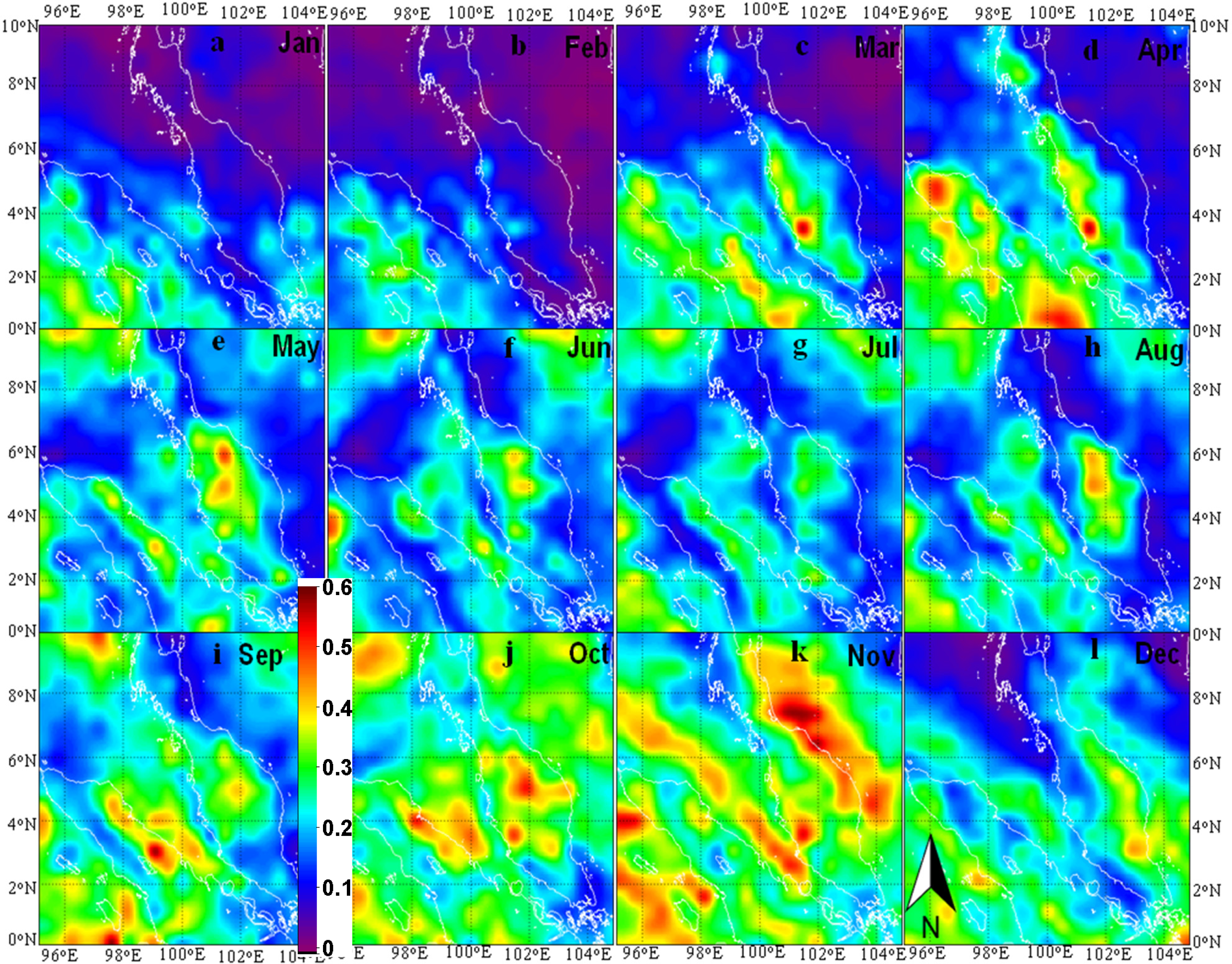Considering the weak correlation between Chl-a and AOT (Figure 5c,d) and the negative correlation between Chl-a and RR (Figure 5e,f), a role of atmospheric dry and wet deposition as nutrient sources in controlling the seasonal Chl-a cycle can be ruled out. The positive correlation between Chl-a and AOT in Area D (Figure 5c,d), where both Chl-a and AOT are low during the SWM (Figure 2f,g,h and Figure 10f,g,h), probably does not reflect direct causation. In other words, a decrease of the AOT during the SWM does not decrease Chl-a, but seasonal winds drive seasonal cycles of Chl-a. Hence, there are two possible sources of nutrients that may drive the seasonal cycle of Chl-a, namely, vertical fluxes from deep layers and/or horizontal fluxes from RD.

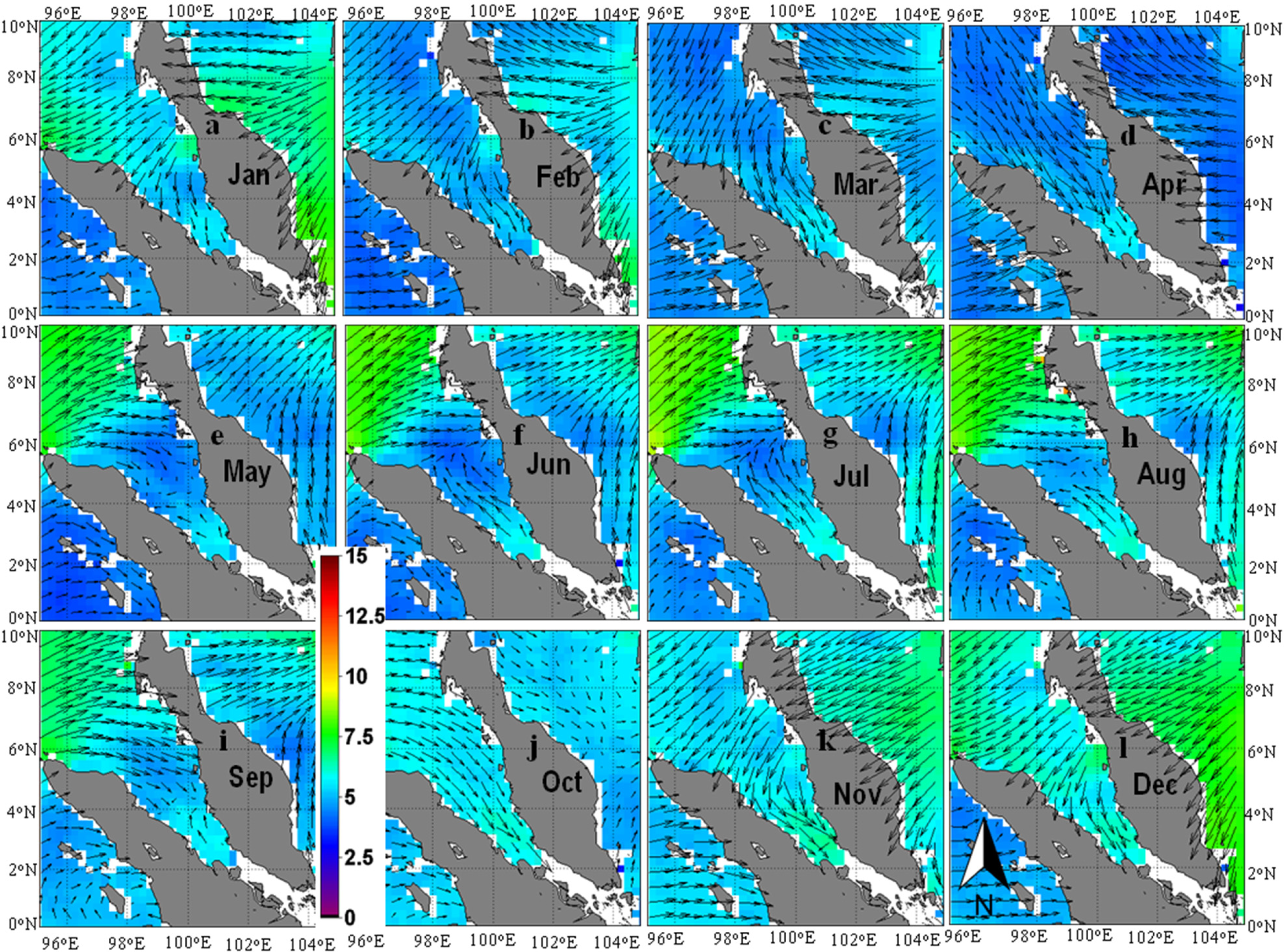
The significant negative correlations between U and Chl-a and between V and Chl-a in the northern region of the SM (Figure 6c–f) reflect the seasonal coupling between high Chl-a and the strong northeasterly winds that occur during the NEM (Figure 11a,b,k,l) and between low Chl-a and the weak southwesterly winds that occur during the SWM (Figure 11e–h). Strong northeasterly winds during the NEM may increase the Chl-a in the northern region of the SM (Figure 2a,b,k,l) in two ways: (1) by increasing the flux of nutrients to surface waters through water column vertical entrainment; and (2) by northwestward horizontal advection of high-Chl-a water from the middle region of the SM via wind-driven Ekman transport [6]. This northwestward Ekman transport probably accounts for the fact that the Chl-a bloom occurs earlier in the middle region (December) compared to in the northern region (January) (Figure 2m). The low Chl-a in the northern region of the SM during the period of weak southwesterly winds may reflect the small amount of water column upward entrainment of nutrients, as well as the southeastward advection of low-Chl-a water from the Andaman Sea via Ekman transport [7].

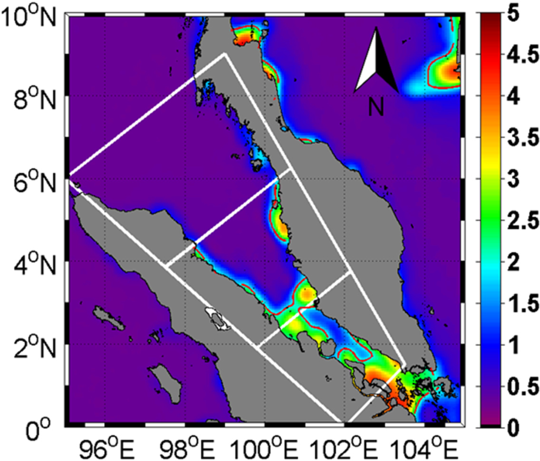
The high Chl-a during the NEM in the middle region of the SM was caused mainly by the increase of Chl-a along the coast of Peninsular Malaysia. One of the possible mechanisms underlying this coastal Chl-a increase is wind-driven coastal upwelling, the evidence for which is the significant negative correlation between V and Chl-a in the coastal area of Peninsular Malaysia (Area C, Figure 6e,f). This coastal upwelling is possible during the NEM, because the middle region of the SM is in the northern hemisphere (∼4°N), and the prevailing winds are alongshore and northwesterly. The positive wind stress curls of >0.04 × 10⁻⁵ Pa·m−1 in Area C (Figure 12a,b,k,l) are also consistent with the occurrence of coastal upwelling during the NEM.

Besides coastal upwelling, high RD in November from Peninsular Malaysia may also have been an important source of allochthonous nutrients from the land. The significant positive correlation between monthly climatological means of RD and Chl-a in the coastal area adjacent to the river estuaries is consistent with this hypothesis (Figure 7b,c). Identifying which factor (upwelling or RD) is more important in causing the Chl-a to be high during the NEM in the middle region of the SM was beyond the scope of this study, because the temporal resolutions of the RD and satellite data were not the same.

The less pronounced seasonal cycle of Chl-a in the southern region of the SM was, to some extent, likely caused by overestimation of SeaWiFS Chl-a. A previous study [6] has mentioned that SeaWiFS Chl-a in turbid coastal areas of the southern region of the SM were an average of about 130% and 480% of the in situ Chl-a during the NEM and SWM, respectively. During the SeaWiFS full mission, the normalized water-leaving radiance at 555 nm (nLw555) was >1 mW·cm⁻²·μm⁻¹·sr⁻¹ (see Figure 13) over half of the southern region of the SM, the implication being that the water in half of the southern region of the SM was turbid. We therefore estimate the Chl-a associated with phytoplankton to be about 3.0 mg·m⁻³ and 1.4 mg·m⁻³ during the NEM and SWM, respectively. These roughly corrected Chl-a in the southern region of the SM made the seasonal cycle and magnitude of Chl-a in the southern region of the SM closely resemble the Chl-a in the middle region of the SM, that is high Chl-a during the NEM, but low during the SWM. The high (low) RR during the NEM (SWM), both from Sumatra and Peninsular Malaysia, was probably one of the factors responsible for causing high (low) Chl-a in the southern region of the SM via the allochthonous flux of nutrients from RD.

3.4. Factors Responsible for the Trends and Interannual Variations of SeaWiFS Chl-a

Significant trends (rate > 0.04 mg·m⁻³·month⁻¹, p < 0.05, Figure 3) of increasing SeaWiFS Chl-a during the SeaWiFS full mission were apparent in the middle and southern regions of the SM. As discussed above, however, SeaWiFS Chl-a in the southern region of the SM very much overestimates in situ Chl-a [6], especially in turbid regions where the nLw555 was >1 mW·cm⁻²·μm⁻¹·sr⁻¹. Because Tan et al. [6] reported in situ Chl-a only during the NEM and SWM, we were unable to estimate the degree of SeaWiFS overestimation of Chl-a in other months during the monsoon transitional seasons. We were therefore unable to estimate the trend of real Chl-a. The trend during the last decade of SeaWiFS Chl-a in the southern region of the SM may also reflect trends of other variables (e.g., inorganic suspended sediment, gelbstoff), which are likely to cause incorrect Chl-a retrieval by the NASA standard ocean color algorithm. The trend of real phytoplankton abundance in the southern region of the SM will therefore remain unclear until the problem of SeaWiFS Chl-a overestimation can be resolved.

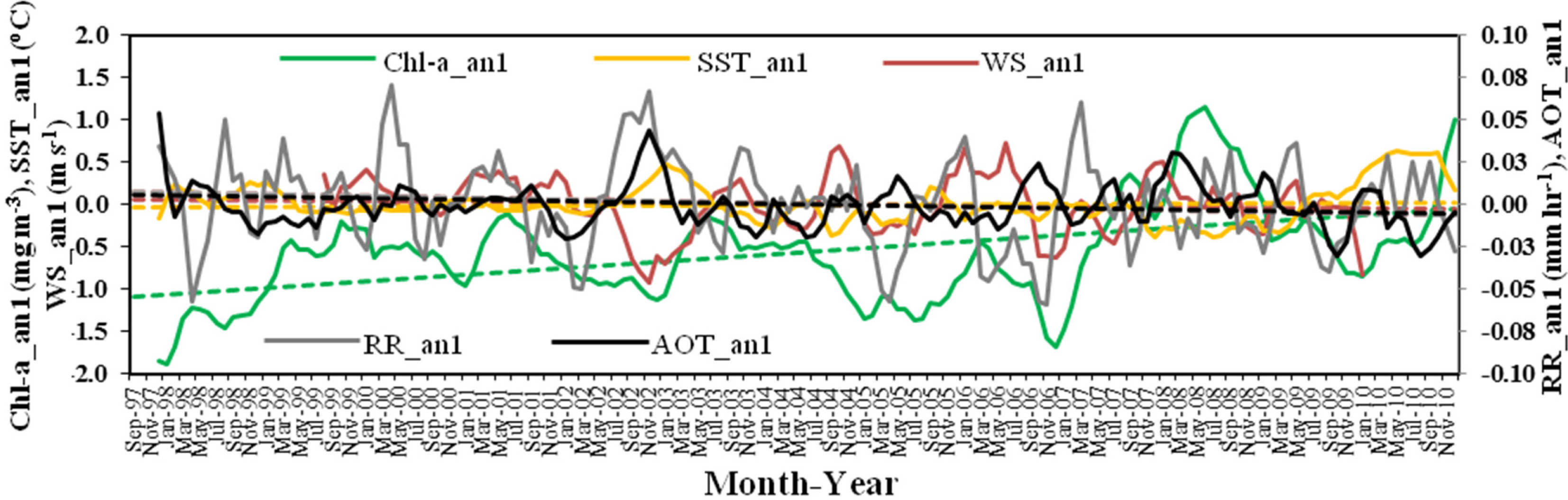
As described above, the trend of increasing SeaWiFS Chl-a in the southern region may be due to increasing trends of other variables that lead to increasing Chl-a retrieved by the NASA ocean color algorithm. The spatial average of Chl-a_an1 in the southern region of the SM significantly increased during the period of this study, as evidenced by the significant correlation (r = 0.43, p < 0.0001, Figure 3b or Figure 14) between SeaWiFS Chl-a_an1 and time. However, environmental variable anomalies of SST_an1, AOT_an1, RR_an1 and WS_an1 showed no significant trends (all r are ≤0.1, p > 0.1, Figure 14). There were no RD data available during the study period, but considering the fact that there was no trend of RR, the possibility that there was a change of RD during the decade associated with the SeaWiFS Chl-a trend can be ruled out. Therefore, other uninvestigated variables, the trends of which were independent of the trends of the investigated environmental variables, may have been responsible for the trend of increasing SeaWiFS Chl-a in the southern region of the SM.

Among undefined variables responsible for the observed trend of increasing SeaWiFS Chl-a in the southern region are increasing nutrient concentrations due to fertilizer use [30] and/or mangrove degradation/land deforestation [31], which may lead to increases of both phytoplankton and inorganic suspended matter. Further research, including studies of changes in land use, land-cover and socio-agricultural issues, is definitely needed to understand land-sea interactions, which may be responsible for changes in the marine environment (including SeaWiFS Chl-a) of the southern region of the SM.

Unlike the southern region, most of the middle region of the SM was characterized by low turbidity, as indicated by the nLw555 of <1 mW·cm⁻²·μm⁻¹·sr⁻¹. Therefore, a significant trend of increasing SeaWiFS Chl-a can be considered to be largely due to a trend of increasing phytoplankton abundance. However, none of the investigated variables in the middle region showed remarkable trends (data not shown). Therefore, like the southern region of the SM, the trend of increasing SeaWiFS Chl-a in the middle region of the SM was probably associated more with variables whose trends were independent of the investigated variables, such as increasing surface nutrient concentrations due to increased use of fertilizer [30].

In regard to interannual variations, the northern region of the SM seemed to be more responsive to ENSO (r = 0.26, p < 0.01) than to IOD (r = 0.18, p < 0.05, Table 1). The correlations between positive climate changes and Chl-a increases were nevertheless both statistically significant, the implication being that during both El Niño (positive Nino3.4) and positive IOD events, Chl-a in the northern region tended to increase significantly. Among the investigated environmental variables, AOT is likely the principal factor responsible for interannual variations of Chl-a in the northern region, as evidenced by the significant positive correlation between Chl-a_an2 and AOT_an2 (r = 0.25, p < 0.05). It is well known that both El Niño and positive IOD events cause severe droughts in Indonesia, and those droughts are frequently followed by wildfires [11,12]. Dry atmospheric deposition of macro- and/or micro-nutrients from aerosols as a result of wildfires probably fertilized the northern region of the SM. This fertilization is a likely explanation for the significant correlation between AOT and Chl-a in the northern region [12]. RR arises as one of the most important variables in causing interannual variations of Chl-a in the northern region (r = 0.18, p < 0.05 for Chl-a_an2 versus RR_an2). Seemingly, the mechanism by which RR increases Chl-a in the northern region during both El Niño and positive IOD conditions is related to the intensification of wet atmospheric deposition, due to high concentrations of atmospheric aerosols during both El Niño and positive IOD conditions.

In the middle region of the SM, Chl-a interannual variations were more responsive to the IOD than to ENSO events. A significant positive correlation (r = 0.31, p < 0.01) between the DMI and SeaWiFS Chl-a_an2 in the middle region implies that during positive IOD conditions (positive DMI), Chl-a in the middle region tended to increase. Among the explanatory variables, AOT_an2 and RR_an2 appear to be the main causes of interannual variations of Chl-a in the middle region, as evidenced by significant correlations between AOT_an2, RR_an2 and Chl-a_an2 (r >= 0.19, p < 0.05) and, to some degree, by their co-variations (Figure 4a–c, green lines). The same mechanism operative in the northern region also applies in the middle region. Droughts occur during positive IOD events, and both dry and wet atmospheric deposition of aerosols from wildfires likely elevate surface nutrient concentrations.

The climatic anomaly of ENSO seemed to be more important in causing interannual variations of Chl-a in the southern region of the SM (Figure 4a), as evidenced by the significant negative correlation between Nino3.4 and SeaWiFS Chl-a_an2 (r = −0.52, p < 0.01). However, note that this interannual variation of Chl-a may not be associated only with interannual variations of phytoplankton abundance; it may also reflect the problematic SeaWiFS Chl-a retrieval, as described above. Among the obvious interannual variations of SeaWiFS Chl-a in the southern region were the low Chl-a in 1997 and during the period from 2004 to 2006 (see both Figures 3b and 4a, red lines). Those two periods were times of severe drought in Peninsular Malaysia associated with El Niño events. In fact, RR during those periods was anomalously low (Figure 4b, red line). The significant positive correlation (r = 0.17, p < 0.05) between SeaWiFS Chl-a_an2 and RR_an2 is also noteworthy. This correlation implies that droughts during El Niño events are likely to reduce RR and, hence, RD, and their reduction further reduces nutrient and sediment loads from the land. This effect will ultimately reduce total suspended matter, both in the form of phytoplankton and inorganic suspended matter, the result being low SeaWiFS Chl-a retrieval in the southern region of the SM during El Niño years. The impacts of large-scale climatic anomalies on seemingly real phytoplankton abundance in the southern region of the SM were hence unresolved in this study, for the reasons described above.

Development of a local Chl-a algorithm, especially a semi-analytical algorithm that allows separate retrievals of not only Chl-a, but also of other in-water constituents, will be necessary for the quantification of the spatial and temporal variations of real Chl-a, not only in the southern region of the SM, but also in optically complex turbid coastal waters [32]. In addition, instead of satellite-derived Chl-a, satellite-derived fluorescence line height (FLH, but since 1999 (2002) for MODIS-Terra (Aqua)) may be a better variable to use for tracing the seasonal cycles, interannual variations and long-term trends of real phytoplankton abundance, because satellite-retrieved FLH represents real phytoplankton better than satellite-retrieved Chl-a in waters optically influenced by inorganic suspended matter and gelbstoff [33].

4. Conclusions

Despite the small size of the SM, there exist within the SM obvious meridional differences in terms of SeaWiFS Chl-a seasonal cycles, interannual variations and decadal-scale trends, as well as the impacts of the principal causes of this variability. Over the entire SM, Chl-a is high (low) during the NEM (SWM), the likely predominant causes being wind-driven vertical mixing in the north and wind-driven coastal upwelling and, possibly, RD in the middle region. Because of quality issues associated with SeaWiFS Chl-a and the absence of wind field retrieval, the principal factor responsible for Chl-a variations in the southern region was unresolved in this study. In addition, phytoplankton tend to bloom later in the northern region, probably because of coastal upwelling in the middle region and northwestward Ekman transport from the middle to the northern regions during the NEM.

In terms of interannual variations, SeaWiFS Chl-a responded negatively to ENSO in the southern region, but positively to IOD in the middle region and positively to both ENSO and IOD in the northern region of the SM. Seemingly dry (by AOT, mainly) and wet (by RR) atmospheric deposition during El Niño and/or positive IOD are responsible for elevating surface nutrient concentrations, the result being an increase of Chl-a during positive IOD and/or El Niño conditions in the northern and middle regions of the SM. The predominant factor causing SeaWiFS Chl-a to decrease in the southern region was a decrease of RR, probably associated with drought during El Niño conditions.

Among the three regions, the southern region of the SM showed the most pronounced trend of increasing SeaWiFS Chl-a during the SeaWiFS full mission period. A moderately increasing trend of SeaWiFS Chl-a was also apparent in the middle region. The factors responsible for the trend of increasing SeaWiFS Chl-a in the middle and southern regions are unclear, but were probably related to other environmental variables, the variations of which were independent of the variations of variables investigated in this study.

The spatial and temporal variations of seemingly real phytoplankton abundance in the southern region, however, remain unclear, because of quality issues associated with the SeaWiFS Chl-a. In future studies, we therefore recommend the application of a reliable local Chl-a algorithm and the use of satellite-derived fluorescence as prerequisites for discerning spatio-temporal variations of seemingly real Chl-a, not only in the southern region of the SM, but also in other optically complex turbid waters.