Identifying Changing Snow Cover Characteristics in Central Asia between 1986 and 2014 from Remote Sensing Data

Abstract

Central Asia consists of the five former Soviet States Kazakhstan, Kyrgyzstan, Tajikistan, Turkmenistan, and Uzbekistan, therefore comprising an area of ~4 Mio km². The continental climate is characterized by hot and dry summer months and cold winter seasons with most precipitation occurring as snowfall. Accordingly, freshwater supply is strongly depending on the amount of accumulated snow as well as the moment of its release after snowmelt. The aim of the presented study is to identify possible changes in snow cover characteristics, consisting of snow cover duration, onset and offset of snow cover season within the last 28 years. Relying on remotely sensed data originating from medium resolution imagers, these snow cover characteristics are extracted on a daily basis. The resolution of 500–1000 m allows for a subsequent analysis of changes on the scale of hydrological sub-catchments. Long-term changes are identified from this unique dataset, revealing an ongoing shift towards earlier snowmelt within the Central Asian Mountains. This shift can be observed in most upstream hydro catchments within Pamir and Tian Shan Mountains and it leads to a potential change of freshwater availability in the downstream regions, exerting additional pressure on the already tensed situation.

1. Introduction

Freshwater availability in Central Asia depends on the occurrence and amount of snowfall (e.g., [1,2,3]). Climate change as well as human interaction have altered the water balance of the region, causing serious water shortages, retreat of glaciers, desertification, and the drying-up of the Aral Sea [4,5,6,7,8,9]. Population growth and the intensifying demand on more water for irrigation and the production of hydropower stand in contrast to the decline of the resource [10,11], causing also political tensions to arise [8,12]. Against this background a detailed analysis of processes like changing snow cover duration, onset, or melt of snow-covered areas becomes more important. 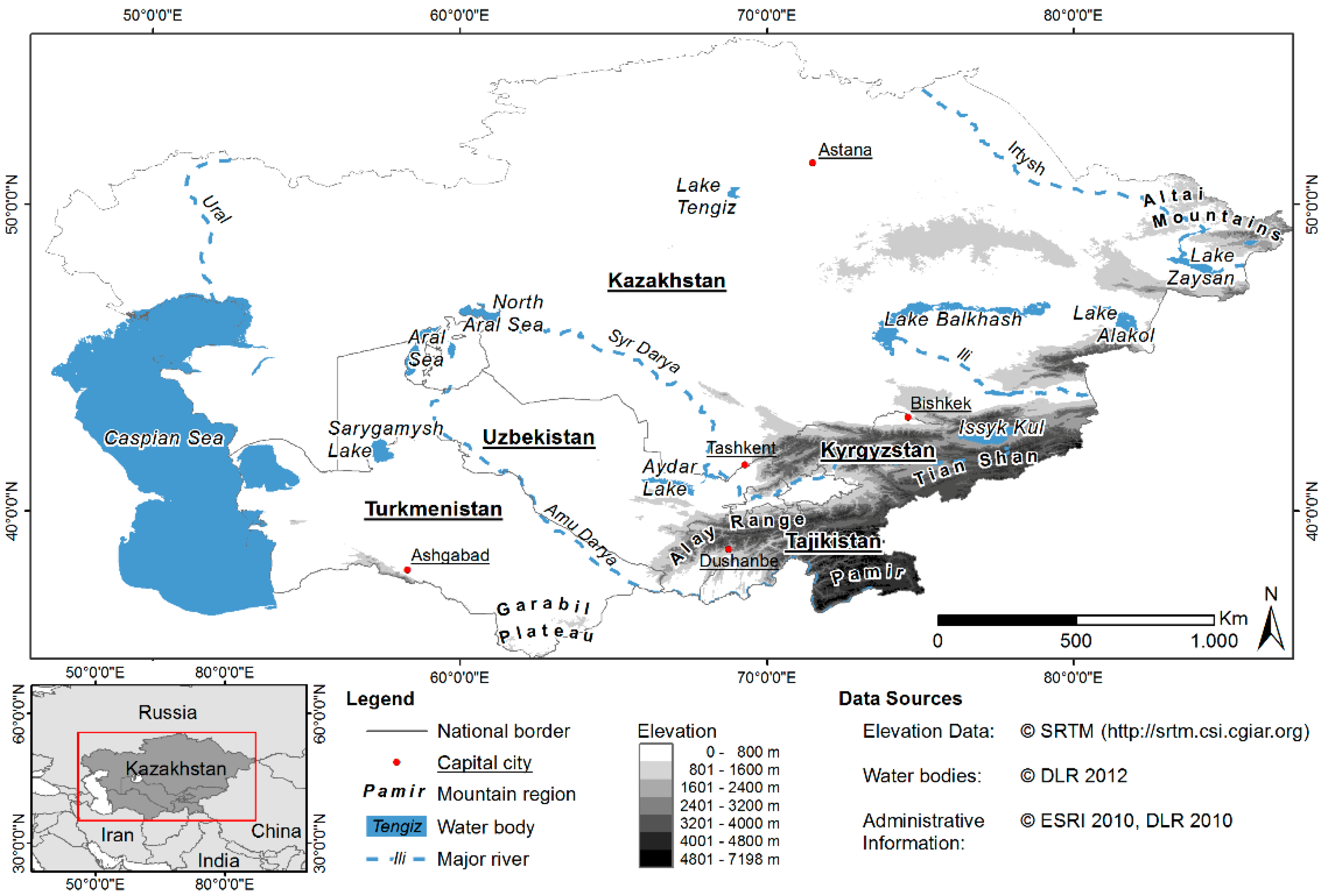Table 1 includes some basic information about the study region. The economy of Central Asia depends largely on agriculture, namely cotton and grains [13]. River runoff of Amu Darya and Syr Darya is of particular importance especially in Tajikistan, Turkmenistan, and Uzbekistan as these countries irrigate large portions of their arable land.

The aim of the presented study is to answer the question how snow cover has changed in the upstream catchments of Central Asia. It is the mountainous region of Pamir and Tian Shan (Figure 1) where the origins of the two most important streams of Central Asia—Syr Darya and Amu Darya—are located. These rivers form the lifelines of the whole region [12] and therefore, information about ongoing changes on a sub-catchment scale is desirable. The presented results tie to an earlier research about Central Asian snow cover characteristics between 2000 and 2011 [14] and follow a similar study about snow cover changes between 1986 and 2008 in the Amu Darya river catchment [15]. The results of the latter study already show a decreasing trend in Snow Cover Duration (SCD) especially for the high elevation regions with a shift towards earlier snow cover start and melt. Therefore, the secondary aim of our study is to investigate whether the findings of [15] can be confirmed also for the Syr Darya catchment and whether the results for Amu Darya would conform. This is of particular interest as especially the delineation of snow cover from Advanced Very High Resolution Radiometer (AVHRR) data can pose a challenge.

Table 1. States of Central Asia—basic information.

Country	Area (km2) *	Population *	GDP (Per Capita in US $) *	Irrigated area (% of Arable Land) **
Kazakhstan	2,724,900	16,724,000	14,570	6%
Kyrgyzstan	198,974	5,700,000	1343	3%
Tajikistan	141,949	8,354,000	988	35%
Turkmenistan	488,962	5,796,000	6602	31%
Uzbekistan	432,544	29,893,000	2123	89%

* as estimated for 2014, data source [16]; ** as estimated for 2010, data source [13].

Table 1. States of Central Asia—basic information.

Country	Area (km2) *	Population *	GDP (Per Capita in US $) *	Irrigated area (% of Arable Land) **
Kazakhstan	2,724,900	16,724,000	14,570	6%
Kyrgyzstan	198,974	5,700,000	1343	3%
Tajikistan	141,949	8,354,000	988	35%
Turkmenistan	488,962	5,796,000	6602	31%
Uzbekistan	432,544	29,893,000	2123	89%

* as estimated for 2014, data source [16]; ** as estimated for 2010, data source [13].

Figure 1. Overview of Central Asia.

Figure 1. Overview of Central Asia.

Techniques for mapping snow from remotely sensed data have been developed since the 1960s when TIROS-1 (Television and InfraRed Observation Satellite) allowed for snow cover detection [17]. Methods and sensors have been improved continuously since that time. Especially when it comes to snow cover mapping for larger regions and longer time series, remote sensing constitutes a reliable and unrivaled data source. The reflection of a snow-covered surface in the visible part of the spectrum can reach 95% and drops near zero in the short-wave infrared. These values may differ considerably depending on grain size and age of the snow crystals as well as the liquid water content. Details about the challenges to map snow cover and discriminate between clouds and snow have been discussed extensively in literature. The interested reader should refer to [18,19,20,21] for more information.

2. Data Sources

We rely on the longest possible time series of medium resolution remote sensing data that is available on a daily basis and analyze AVHRR and Moderate Resolution Imaging Spectroradiometer (MODIS) data between 1986 and 2014. Spatial and temporal resolutions of these sensors are consistent with the demands for satellite-based data products for climate research formulated by the Global Climate Observing System (GCOS) [22]. Table 2 gives on overview of existing and upcoming sensors to map snow from the reflective part of the spectrum. Though there are additional sensors like ATSR/AATSR or MERIS available, the need for long-term daily observations limits the selection of input data for the presented study to AVHRR and MODIS. The suitability of earth observation data originating from the reflective part of the spectrum for snow mapping has repeatedly been confirmed in various studies [18,21,23,24,25] and the remoteness and sheer size of the study region - combined with the requirement to measure the snow cover extent on a daily basis and over multiple years - leaves not too many alternatives to optical satellite data.

It is possible to map snow cover using Synthetic Aperture Radar (SAR) data, but several limitations prevent their consideration for the presented study: Snow cover only becomes visible under wet snow conditions [21,26], and the temporal resolution of SAR sensors is typically too low to derive daily snow cover information for an area as big as the study region of Central Asia (11, 24, 35 days for TerraSAR-X, RADARSAT, Envisat/ASAR data, respectively). Additionally, the time series of available SAR data only ranges back until 1995 (RADARSAT). Passive Microwave (PM) data would be another alternative [27,28,29,30,31], but the spatial resolution is way too coarse to derive accurate measurements (pixel size of PM is usually around 25km, e.g., GlobSnow Snow Water Equivalent (SWE) product [32]). Additionally, PM data is not suited to detect snow cover in mountainous regions [18,21,32]—the most important part of the study region Central Asia as the majority of available freshwater is generated here by snowmelt.

Table 2. Remote Sensing instruments used to map snow cover from the reflective part of the spectrum.

Satellite(s)—Instrument(s)	Operational since/until	Revisit Time	Spatial Resolution	Swath Width
Landsat MSS/TM/ETM+/OLI	1972/Today	16–18 days	30–100 m	185 km
Terra, Aqua-MODIS	2000/Today	Twice per day	250–1000 m	2330 km
TIROS/NOAA/Metop AVHRR	1978/Today	At least daily	1100 m	2400 km
Envisat/AATSR	2002/2012	2–3 days	1000 m	500 km
Envisat/MERIS	2002/2012	2–3 days	300 m	1150 km
ERS-2/ATSR-2	1995/2011	2–3 days	1000 m	512 km
Sentinel 2	to be launched in 2015	3–5 days	10–60 m	290 km
Sentinel 3-OLCI/SLSTR	to be launched in 2015	1–2 days	300–500 m	1270 km
Suomi-NPP-VIIRS	2011/Today	Daily	375–750 m	3040 km

Sources: [33,34,35,36,37,38,39,40,41].

Table 2. Remote Sensing instruments used to map snow cover from the reflective part of the spectrum.

Satellite(s)—Instrument(s)	Operational since/until	Revisit Time	Spatial Resolution	Swath Width
Landsat MSS/TM/ETM+/OLI	1972/Today	16–18 days	30–100 m	185 km
Terra, Aqua-MODIS	2000/Today	Twice per day	250–1000 m	2330 km
TIROS/NOAA/Metop AVHRR	1978/Today	At least daily	1100 m	2400 km
Envisat/AATSR	2002/2012	2–3 days	1000 m	500 km
Envisat/MERIS	2002/2012	2–3 days	300 m	1150 km
ERS-2/ATSR-2	1995/2011	2–3 days	1000 m	512 km
Sentinel 2	to be launched in 2015	3–5 days	10–60 m	290 km
Sentinel 3-OLCI/SLSTR	to be launched in 2015	1–2 days	300–500 m	1270 km
Suomi-NPP-VIIRS	2011/Today	Daily	375–750 m	3040 km

Sources: [33,34,35,36,37,38,39,40,41].

2.1. AVHRR Data

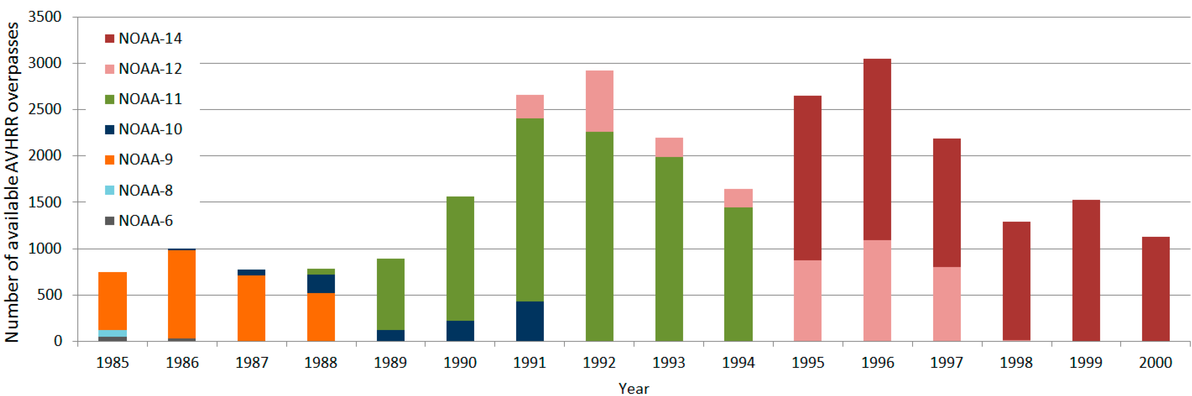
The AVHRR data were acquired from the National Oceanic and Atmospheric Administration’s (NOAA) Comprehensive Large Array-data Stewardship System (CLASS) [42]. All available Level 1B (quality controlled with included, but not applied information about calibration and geolocation) data were downloaded, comprising AVHRR generations 1, 2, and 3. Figure 2 illustrates the varying number of scenes per sensor and year (total number of scenes: ~27,000). The amount of available data turned out to be irregular as especially during the late 1980s many scenes were missing. AVHRR sensors observe the Earth in 5 spectral bands (4 for AVHRR generation 1). Table 3 gives on overview of the sensor characteristics of all AVHRR channels, including also those not used in the presented study. Generation 1 data (NOAA-6, -8, and -10) only contributes a few hundred scenes for the years before 1992. The discrimination between clouds and snow is a challenging task, and for AVHRR generation 1 with only one thermal infrared channel the quality of snow cover classification deteriorates significantly when compared to generations 2 and 3 [43,44]. The format of the Level 1B data is Local Area Coverage (LAC), whose record length is limited to ten minutes.

Figure 2. AVHRR data acquired from NOAA CLASS.

Figure 2. AVHRR data acquired from NOAA CLASS.

Table 3. Spectral band widths (µm) and operational phases of AVHRR sensors.

Channel *	TIROS-N	NOAA-6, -8, -10	NOAA-7, -9, -11, -12, -14 **	NOAA-15, -16, -17, -18, -19
1 (VIS)	0.55–0.90	0.58–0.68	0.58–0.68	0.58–0.68
2 (NIR)	0.725–1.10	0.725–1.10	0.725–1.10	0.725–1.00
3A (MIR)	-	-	-	1.58–1.64
3B (MIR)	3.55–3.93	3.55–3.93	3.55–3.93	3.55–3.93
4 (TIR)	10.50–11.50	10.50–11.50	10.30–11.30	10.30–11.30
5 (TIR)	-	-	11.50–12.50	11.50–12.50
Operational	May 1978–January 1980	June 1979–September 1991	August 1981–October 2002	October 1998–present

* VIS: Visible spectrum; NIR: Near infrared; MIR: Medium infrared; TIR: Thermal infrared; ** NOAA-13 never became operational due to a spacecraft power supply malfunction after launch. All information taken from [45,46].

Table 3. Spectral band widths (µm) and operational phases of AVHRR sensors.

Channel *	TIROS-N	NOAA-6, -8, -10	NOAA-7, -9, -11, -12, -14 **	NOAA-15, -16, -17, -18, -19
1 (VIS)	0.55–0.90	0.58–0.68	0.58–0.68	0.58–0.68
2 (NIR)	0.725–1.10	0.725–1.10	0.725–1.10	0.725–1.00
3A (MIR)	-	-	-	1.58–1.64
3B (MIR)	3.55–3.93	3.55–3.93	3.55–3.93	3.55–3.93
4 (TIR)	10.50–11.50	10.50–11.50	10.30–11.30	10.30–11.30
5 (TIR)	-	-	11.50–12.50	11.50–12.50
Operational	May 1978–January 1980	June 1979–September 1991	August 1981–October 2002	October 1998–present

* VIS: Visible spectrum; NIR: Near infrared; MIR: Medium infrared; TIR: Thermal infrared; ** NOAA-13 never became operational due to a spacecraft power supply malfunction after launch. All information taken from [45,46].

2.2. MODIS Daily Snow Cover Products MOD10A1/MYD10A1

The MODIS daily snow cover products MOD10A1 and MYD10A1 were acquired from the National Snow and Ice Data Center (NSIDC, [47]) for the years 2000 to 2014. Based on the snowmap algorithm which was developed especially for MODIS [38], snow cover information is made available for the whole globe on a daily basis and for both platforms: Aqua (MYD10A1), and Terra MODIS (MOD10A1). The snowmap algorithm is based on the Normalized Difference Snow Index (NDSI) (Equation (1)) developed by [48] in 1984:

$$NDSI=\frac{(R_{VIS}-R_{IR})}{(R_{VIS}+R_{IR})}$$

(1)

where R_VIS and R_IR stand for the reflection in the visible and (medium-) infrared spectrum, respectively. For Terra MODIS, bands 4 (VIS) and 6 (IR) are used for the calculation of the NDSI. The Aqua MODIS product relies on bands 4 and 7, as band 6 is non-functional [49]. The NDSI exploits the typical spectral characteristics of snow: High reflection in the visible part of the spectrum, which drops near zero in the infrared region. An NDSI higher 0.4 is a good indicator for snow [38,50]. The snowmap algorithm uses additional tests to increase the accuracy of the snow cover product and to prevent misclassifications over water bodies and forested areas (10% minimum reflectance threshold in band 4, lower NDSI threshold over forested regions). Fractional snow cover information per pixel is also included in the MOD10A1 and MYD10A1 product. The details about the fractional snow cover component can be found in [51]. They are not reviewed here as only the binary snow information is used for the presented study. The accuracy of the final MODIS daily snow cover product reaches 93% [52] as it was confirmed by various independent studies throughout the world [50,53,54,55,56]. Snow depth [57], land cover type [52], and the transition zone between snow covered and snow free area [58] can compromise the accuracy. Additionally, the accuracy is given only for clear sky pixels. It is know from several studies that the MODIS cloud detection scheme tends to overestimate clouds due to misinterpretation of snow [59,60].

For the presented study, a total number of ~76,000 MODIS snow cover datasets (MOD10A1/MYD10A1) were used. The products provide a thematic layer containing classes for snow, snow-free land, sea ice, water, and clouds. This thematic information is not available from the raw AVHRR data and has to be derived before snow cover parameters used to analyze snow cover trends can be produced.

3. Processing Methods and Validation Results

Several processing steps are required to analyze the time series of snow cover data from Central Asia for possible long-term changes. The very first step is the preprocessing and classification of snow cover from AVHRR data. Step number two will deal with the post-processing of the time series in order to estimate snow cover conditions below clouds. Third, snow cover parameters like Snow Cover Duration (SCD), Early Season SCD (SCD_ES), and Late Season SCD (SCD_LS) have to be calculated. Finally, a validation of the processed datasets is necessary. The following subchapters will describe every step in detail, beginning with the processing of AVHRR data. The interpretation and discussion of the results will follow in Section 4 and Section 5.

3.1. AVHRR (Pre-)Processing

Details about the acquired AVHRR data have already been presented in Section 2.1: The raw Level 1B LAC data require preprocessing in order to apply geolocation and calibration as well as additional processing to classify the snow covered area. The amount of data (~ 27,000 scenes) demands automated processing as any manual interaction would cause enormous expenditures of work. Several algorithms exist to fulfill the task of automated processing of the full time series: Separation of Pixels Using Aggregated Rating over Canada (SPARC) was used in Canada [24] and in a modified version for Europe [25]. It consists of three cloud tests plus additional snow and thin cirrus tests. The advantage of SPARC is the aggregated rating approach of these test ratings, meaning that every test is independent from each other. The drawback of SPARC however is the need to provide the algorithm with data about the daily skin temperature—information that is not available for Central Asia. Clouds from AVHRR (CLAVR) is another processing routine available for AVHRR [61]. Unfortunately, CLAVR requires surface type maps and monthly climatological fields—again inputs that cannot be provided for the full time series of the analysis.

We rely on the AVHRR Processing Over Land cLoud and Ocean (APOLLO) scheme to facilitate the cloud cover classification and discrimination between clouds and snow. APOLLO does not require any auxiliary inputs and is operational at the German Aerospace Center (DLR) for more than 15 years, processing cloud information for daily Normalized Difference Vegetation Index (NDVI), Sea Surface Temperature (SST), and Land Surface Temperature (LST) products for Europe [62,63]. Though already developed in the late 1980s, extensions for snow and ice mapping [43] and additional updates to improve the accuracy of the cloud detection were added [63] that qualify APOLLO for the task to classify snow cover in Central Asia. The procedure is two-parts: calibration and geolocation are applied to the raw AVHRR data relying on Terascan software [64], ensuring sophisticated calculation of channel 1 and 2 Top Of Atmosphere (TOA) reflectance as well as channel 4 and 5 Brightness Temperatures (BT). A continuous post-launch calibration is required for AVHRR to remove all spurious trends that originate from sensor degradation [46]. Terascan automatically relies on continuously updated calibration coefficients to answer to these requirements. Channel 3 is calibrated to simple radiances as APOLLO expects the reflective part of channel 3 as input. This parameter is most useful for separating clouds and snow [34] and is calculated within APOLLO from channel 3 radiances and channel 4 BT [43].

Figure 3. AVHRR Processing Over Land, cLoud and Ocean (APOLLO) snow and ice detection scheme (R_C3: Reflectance in channel 3; D_C1-C2: Difference between channel 1 and channel 2; T₄: brightness temperature in channel 4; DVT: Dynamic visible threshold; R21T: ratio between channel 1 and channel 2—cloud test; R31T: Ratio between channel 3 and channel 1; T45T: Difference between brightness temperatures of channels 4 and 5); all information taken from [43].

Figure 3. AVHRR Processing Over Land, cLoud and Ocean (APOLLO) snow and ice detection scheme (R_C3: Reflectance in channel 3; D_C1-C2: Difference between channel 1 and channel 2; T₄: brightness temperature in channel 4; DVT: Dynamic visible threshold; R21T: ratio between channel 1 and channel 2—cloud test; R31T: Ratio between channel 3 and channel 1; T45T: Difference between brightness temperatures of channels 4 and 5); all information taken from [43].

Part two of the AVHRR processing chain involves the classification of snow-covered surfaces from the preprocessed input coming from Terascan. The extension for ice and snow detection [43] constitutes the basis of this step. The background is illustrated in Figure 3: Several successive threshold tests are applied to APOLLO’s cloud cover classification to discriminate between clouds and snow (Details about the cloud detection algorithm can be found in [44]). All available AVHRR channels are included but only those pixels are processed that provide enough sunlight (pixels with solar zenith angels greater than 80° are excluded). The Dynamic Visible Threshold (DVT) test, the ratio between channel 2 and channel 1 reflectance (R21T), and the temperature difference between channel 4 and channel 5 (T45T) are cloud tests and they are especially susceptible to confusions between clouds and snow. In the extension, a channel 3 threshold test is added to validate the cloud flagged pixels. The final product consists of a thematic layer including classes for snow, snow-free land, sea ice, water, and clouds. These classes are comparable to those available from the operational MODIS snow cover products [38], allowing for a combination of both datasets.

After the preprocessing not all of the acquired AVHRR scenes contained valid data. Some of the datasets were corrupted; others consisted nearly completely of pixels with nighttime observations where snow cover monitoring is not possible. Around 20,300 out of the 27,000 initial scenes could be processed successfully.

3.2. Estimation of Snow Cover Status below Clouds

The biggest problem for analyzing daily snow cover time series is cloud coverage. Cloud cover percentage in Central Asia reaches more than 70% in winter months [14]. Figure 4 depicts the number of cloud covered days for the hydrological year 2003/2004 (1 September 2003 to 31 August 2004) as derived from MOD10A1. The north as well as the mountainous regions to the south and southeast is affected most severely, hindering a direct assessment of snow cover status for up to 200 days per year. Therefore, a stepwise cloud interpolation routine is applied to the complete time series of AVHRR and MODIS snow cover maps in order to completely remove the compromising effect of clouds. The same procedure was applied for the earlier study in Central Asia [14] as well as for an analogous study in Europe [43]. Additionally, a similar cloud removal routine was applied by [65] also for Central Asia. Therefore, the applied methods will be summarized in a very quick manner only.

Figure 4. Number of cloud covered days during the hydrological year 2003/2004 as derived from MODIS daily snow cover products (MOD10A1).

Figure 4. Number of cloud covered days during the hydrological year 2003/2004 as derived from MODIS daily snow cover products (MOD10A1).

Two different types of techniques are applied to the daily snow cover maps: temporal and spatial interpolation. Temporal interpolation exploits the fact that clouds are dynamic objects. By combining observations from different time steps the effect of clouds can be reduced. For the presented study, we combine all observations from the same date first (Aqua and Terra in the case of MODIS, all valid NOAA satellites and passes in the case of AVHRR). An interpolation covering three successive days follows second. The third step is a spatial interpolation technique, using a Digital Elevation Model (DEM) of the study region to find upper and lower snowlines. Shuttle Radar Topography Mission (SRTM) data was used as data source for the DEM [66]. The method was developed by [67]. The upper snow line represents the elevation where all cloud-free pixels are classified as snow. Above this altitude, all cloud-covered pixels can also be assumed snow-covered—given a certain overall cloud cover percentage is not reached. The lower snowline on the other hand identifies the altitude below which all cloud-free pixels are also snow-free. Once determined, all cloud-covered pixels below the lower snowline can be assumed snow-free. The snowline method exploits the fact that snow cover increases with elevation: In mountainous regions, the mean snow cover duration increases by ~4 days per 100 m altitude [14,67,68]. For the presented study, only scenes with less than 30% overall cloud coverage are processed by this step. Finally, a third temporal interpolation step is added, involving the complete time series to remove the remaining cloud flags: If a pixel is covered by clouds, the algorithm is jumping back and forth in time until a cloud free condition is found. Figure 5 summarizes all processing steps applied to the time series of daily snow cover data.

All these steps reduce the accuracy of the initial snow cover product. Especially during fall and spring, snow cover can constitute a very dynamic land cover feature, sometimes changing quickly from one day to another. Combining several dates of observation can introduce errors so especially the last step can turn out to be problematic (therefore it is located at the very end of the interpolation chain in Figure 5). However: As the intention of the study is to analyze SCD, SCD_ES, and SCD_LS all data gaps must be removed from the time series in order to calculate these parameters. Gaps of up to 60% of the whole time series would not allow for any useful analysis of the results. Comparing several hydrological years would be impossible.

Figure 5. Cloud interpolation steps applied to the time series of daily snow cover data.

Figure 5. Cloud interpolation steps applied to the time series of daily snow cover data.

3.3. Calculation of Snow Cover Parameters SCD, SCD_ES, and SCD_LS

The cloud free daily snow cover maps generated during the preprocessing of AVHRR and cloud interpolation steps form the basis for the calculation of snow cover parameters SCD, SCD_ES, and SCD_LS. SCD is calculated according to Equation (2):

$$SCD={\displaystyle \sum _{i=0}^n(S_i)}$$

(2)

where n is the number of days for the respective year (usually 365; 366 for leap years), and S_i is the binary snow cover information (1 = snow, 0 = snow free) for day i. SCD_ES and SCD_LS base on the same equation, though the number of days differs: For SCD_ES, the SCD between 1 September and 15 January of the next calendar year is calculated while for SCD_LS the SCD between 16 January and 31 August is derived from the time series. The equation, however, is identical with Equation (2). Similar methods were used by [69] to derive SCD and two parameters described as Snow Cover Onset Date (SCOD) and Snow Cover Melt Date (SCMD). The problem with SCOD and SCMD is that by defining a fixed date as onset or offset of the snow cover season, intermediate snowmelt processes cannot be considered. There is usually not only one single SCOD and SCMD but also multiple such dates per season. By defining the parameters SCD_ES and SCD_LS and basing them on Equation (2), this problem can be avoided.

There are many studies from various regions in the world where SCD has been derived using Equation (2) or a similar approach. In [70] SCD was investigated for Canada to analyze the snow cover variability during the spring season because it has a strong effect on the overall Northern Hemisphere snow extent. In [71] the authors discuss the effect of a temperature increase in Europe on SCD in Austria. Prior studies are covering the regions of Poland [72], Europe [68], and the whole world [73], which demonstrate how significant SCD parameters can be to describe possible snow cover changes. Section 4 will outline the results for Central Asia.

3.4. Validation

The validation of the processed snow cover data is an important but challenging task. Especially for the AVHRR time series it is difficult to find appropriate ground truth data that are suitable for validation. The only existing data we know of is the Historical Soviet Daily Snow Depth (HSDSD) data [74]. Unfortunately, the number of available stations is limited to 38 while they only provide data until 1995. To be able to perform a sophisticated validation we had to rely on satellite data as our prime source for reference data. We followed several approaches to assess the quality of the produced snow maps:

A comparison between snow cover maps derived from Landsat is undertaken for several time steps during fall, midwinter, and spring seasons for both mountainous regions and flat plains for different years between 1990 and 1999. Cloud free level 1 Landsat Thematic Mapper (TM) 5 and Enhanced TM+ (ETM+) 7 data have been acquired from the U.S. Geological Survey (USGS). The technique of facilitating higher resolution Landsat data was already used to assess the quality of the MODIS snow cover product [52,55]. Twenty-three scenes were downloaded, classified using NDSI (Equation (1), using Landsat bands 2 and 5 for R_VIS and R_IR, respectively), and manually corrected. The subsequent Landsat snow maps are resampled to fit the resolution of the AVHRR data.

Figure 6 illustrates the comparison between the AVHRR snow cover maps and the Landsat data. The scene from spring season 1999 is situated in the southern Pamir. We decided to investigate the accuracy of the border region between snow covered and snow free land separately as we already suggested that the accuracy may be worse in these transient snow regions. The APOLLO snow product does not consider fractional snow cover which can be expected in this area and therefore, two separate classes for land and snow are introduced in the comparison and Snow covered/snow free regions within a 2 km buffer zone around the border between the two classes and snow covered/snow free regions more than 2 km away from this border zone. The classes in Figure 6 refer to these zones. “Snow > 2 km − Snow” depicts the snow-covered area outside the 2km buffer that was mapped as snow in both, AVHRR and Landsat snow maps. “Snow < 2 km − Snow” on the other hand refers to the coinciding snow pixels within the 2km zone. A class that is described with unequal land cover types—like “Land < 2 km − Snow” illustrates region where within the 2km buffer, the classification of Landsat differs from the one in AVHRR. Though Figure 6 is only one example out of 23 it represents the overall findings: The errors are highest within the transition zone between snow covered and snow free area. A confusion matrix containing the results of the Landsat accuracy assessment is included in Table 4.

Figure 6. Accuracy assessment of Advanced Very High Resolution Radiometer (AVHRR) snow cover maps using Landsat.

Figure 6. Accuracy assessment of Advanced Very High Resolution Radiometer (AVHRR) snow cover maps using Landsat.

Table 4. Confusion Matrix of Landsat and the AVHRR Processing Over Land, cLoud and Ocean (APOLLO) snow product.

AVHRR Snow Products		Landsat Reference Maps					Total	Users Accuracy
	Snow	Land	Snow < 2 km	Land < 2 km	Water/Ice	Clouds
Snow	56417	1531	0	0	0	0	57948	0.97
Land	2671	222905	0	0	266	0	225842	0.98
Snow < 2 km	0	0	42100	12279	0	0	54379	0.77
Land < 2 km	0	0	22289	50292	0	0	72581	0.69
Water/Ice	0	401	0	0	142	0	543	0.26
Clouds	48925	29713	58288	44883	0	0	181809	N/A
Total	108013	254550	122677	107454	408	0	593102
Produce Accuracy	0.52	0.87	0.34	0.46	0.34	N/A
Overall Accuracy: 62.69%				Clear-sky Accuracy: 90.40%
Khat: 0.52				Clear-sky Khat: 0.84

Table 4. Confusion Matrix of Landsat and the AVHRR Processing Over Land, cLoud and Ocean (APOLLO) snow product.

AVHRR Snow Products		Landsat Reference Maps					Total	Users Accuracy
	Snow	Land	Snow < 2 km	Land < 2 km	Water/Ice	Clouds
Snow	56417	1531	0	0	0	0	57948	0.97
Land	2671	222905	0	0	266	0	225842	0.98
Snow < 2 km	0	0	42100	12279	0	0	54379	0.77
Land < 2 km	0	0	22289	50292	0	0	72581	0.69
Water/Ice	0	401	0	0	142	0	543	0.26
Clouds	48925	29713	58288	44883	0	0	181809	N/A
Total	108013	254550	122677	107454	408	0	593102
Produce Accuracy	0.52	0.87	0.34	0.46	0.34	N/A
Overall Accuracy: 62.69%				Clear-sky Accuracy: 90.40%
Khat: 0.52				Clear-sky Khat: 0.84

The classes “Snow < 2 km” and “Land < 2 km” in Table 4 again refer to the 2 km transition zone between snow covered and snow free area. It is clearly visible from the comparison that the accuracy within this zone is significantly lower than outside. Another important finding is that underestimation of actual snow cover due to clouds reaches ~46%. Mixes between land and snow and vice versa only occur for around 2% of the pixels outside the 2 km zone (and 37% inside the zone), but a huge proportion of Landsat snow and land pixels is classified as cloud cover by APOLLO. Only cloud-free Landsat scenes were chosen for the comparison, but as the AVHRR observations originate from different time points we cannot rule out the possibility that these clouds actually existed at another time of the respective day. It is therefore impossible to assess the absolute overall accuracy of the APOLLO snow maps using Landsat (which is—for the sake of completeness—given in Table 4 with 62.7%). This uncertainty leads us to the calculation of the so-called “Clear-sky accuracy”: Only cloud-free pixels are considered for this parameter. The 93% accuracy of the MODIS snow cover product also refers to this value [52,67]. It reaches 90.4% for the APOLLO snow cover product.

The MOD10A1/MYD10A1 daily snow cover product has been validated by various researchers during several studies throughout the world as already stated in Section 2.2. The clear-sky accuracy was confirmed to reach ~93% and no further validation was accomplished for the presented study in Central Asia. The accuracy of the MODIS snow cover product is higher than the APOLLO snow cover product accuracy. This was expected since the spatial as well as the spectral resolution of MODIS is finer, the geolocation accuracy is higher, and the algorithm to derive snow cover is more up-to-date.

An intercomparison between APOLLO and MOD10A1/MYD10A1 was performed additionally to the Landsat assessment of the APOLLO snow product. As the accuracy of MODIS was confirmed by several independent researchers to be around 93%, a comparison with APOLLO may produce additional findings. This assessment can only be derived for years after 2000 as MODIS was not operational before and therefore, only NOAA-14 data could be validated using this method (see Figure 2). We compared daily snow cover data between 2 February 2010 and 7 April 2000 for the full area of Central Asia (8 MODIS tiles). The agreement of both products varies between 80.1% and 98.8%, with a mean overall agreement of 90.3%. Higher cloud coverage leads to worse agreement between the products: On 24 March cloud cover percentage reached 88% in Central Asia. This is also the date with the lowest overall agreement between MODIS and APOLLO (80.1% agreement of clear sky pixels). Pixels covered by clouds in either of the products are not considered in the statistics. This is due to the fact that the observation times of AVHRR and MODIS vary and therefore, the existence of different cloud patterns is possible within the same calendar date.

Another important validation step is the assessment of the cloud interpolation accuracy. It was already mentioned in Section 3.2 that cloud cover percentage in Central Asia can add up to 70% in some regions. This means that a vast amount of pixels is being reprocessed in order to prepare a cloud free time series of daily data. To assess the accuracy of these data it is difficult to compare the reprocessed products with ground truth information due to the lack of such. Therefore, we simulate artificial clouds into scenes with relatively low cloud coverage, process these scenes with the cloud interpolation scheme (Figure 5), and compare the cloud-cleared scenes with the original versions before they were artificially corrupted with clouds. Doing so, each step within the cloud interpolation chain can be assessed individually. Figure 7 depicts the accuracy of each step (X-axis). The bars illustrate the accuracy of the respective step while the line plot shows how often the step was actually applied to the time series. This frequency is also given in brackets and it clearly demonstrates that step 1, the combination of all observations from the same day clears most (67.7%) of the affected pixels. The step with the highest accuracy (step 3—snowline analysis) is unfortunately only applied to 1.1% of the input data. The accuracy values illustrated in Figure 7 conform with those already analyzed in a similar approach by [65].

Figure 7. Accuracy of cloud interpolation steps as identified from simulating artificial clouds. Accuracy (grey columns), Standard Deviation (black dotted line bars), and frequency of a step being applied to the input data (black continuous line).

Figure 7. Accuracy of cloud interpolation steps as identified from simulating artificial clouds. Accuracy (grey columns), Standard Deviation (black dotted line bars), and frequency of a step being applied to the input data (black continuous line).

When taken all together, the overall accuracy of the whole interpolation chain accounts for 89.8%. Furthermore, when acting on the assumption that the accuracy of the input data is 90% for the APOLLO and 93% for the MODIS snow cover products and the mean cloud cover percentage for Central Asia is 43% (see [14]), the theoretical accuracy of the daily snow cover data constituting the basis for the results presented in the next section accounts for 86.1% and 89.0% for APOLLO and MODIS, respectively. Several uncertainties may cause these estimated values to vary slightly, as cloud cover is more concentrated in winter than summer months. Additionally, the distribution of the actually applied cloud interpolation step on each pixel may shift several percent from scene to scene, also slightly changing the overall accuracy of the respective scene.

4. Results

SCD, SCD_ES, and SCD_LS are calculated for all hydrological years between 1986/1987 and 2013/2014. Derived for entire Central Asia these datasets constitute a large collection of spatial data, which is too extensive to include in this section. Some results of SCD, SCD_ES, and SCD_LS for the years between 2000 and 2012 have been published in [14]. Therefore, only one map containing the mean SCD for the period between 2000 and 2013 is depicted in Figure 8.

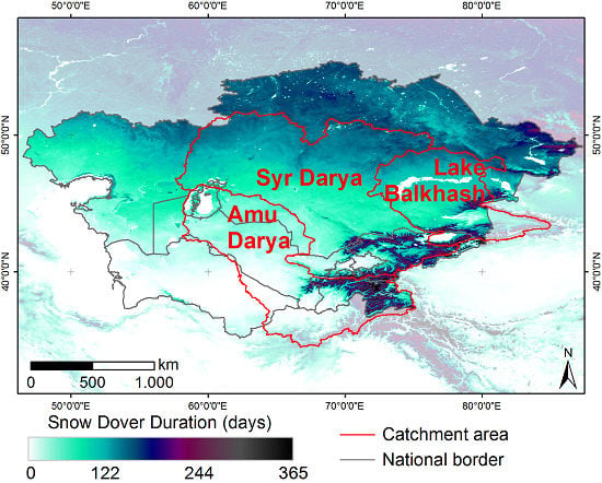
This map illustrates how SCD is distributed in whole Central Asia (Figure 8d) as well as within the single catchment areas (Figure 8a–c): Longest SCD is found within the mountainous region to the south and southeast. It also demonstrates that when analyzing the hydrology of an area, political boundaries do not necessarily coincide with the natural border of a catchment: Amu Darya is covering six different nations: Kazakhstan, Kyrgyzstan, Tajikistan, Turkmenistan, Uzbekistan, and Afghanistan. Even though Afghanistan is not part of the study about snow cover in Central Asia, the part falling within the Amu Darya River catchment is therefore included in the statistics. The same is true for the Lake Balkhash catchment: The upper reaches of the Ili River, which drains into Lake Balkhash, are situated on Chinese territory and also included in the statistics.

Figure 8. Amu Darya (a), Syr Darya (b), and Lake Balkhash (c) with subcatchments and mean Snow Cover Duration between 2000 and 2013. Overview of whole Central Asia (d) with all catchment areas highlighted in red.

Figure 8. Amu Darya (a), Syr Darya (b), and Lake Balkhash (c) with subcatchments and mean Snow Cover Duration between 2000 and 2013. Overview of whole Central Asia (d) with all catchment areas highlighted in red.

The subcatchments of Amu Darya (Figure 8a) and Syr Darya (Figure 8b) have been divided into upper-, middle-, and down-stream catchments in order to provide clearer results within this section. These zones are highlighted in different colors in Figure 8. Lake Balkhash (Figure 8c) only consists of three catchment zones and has not been differentiated any further.

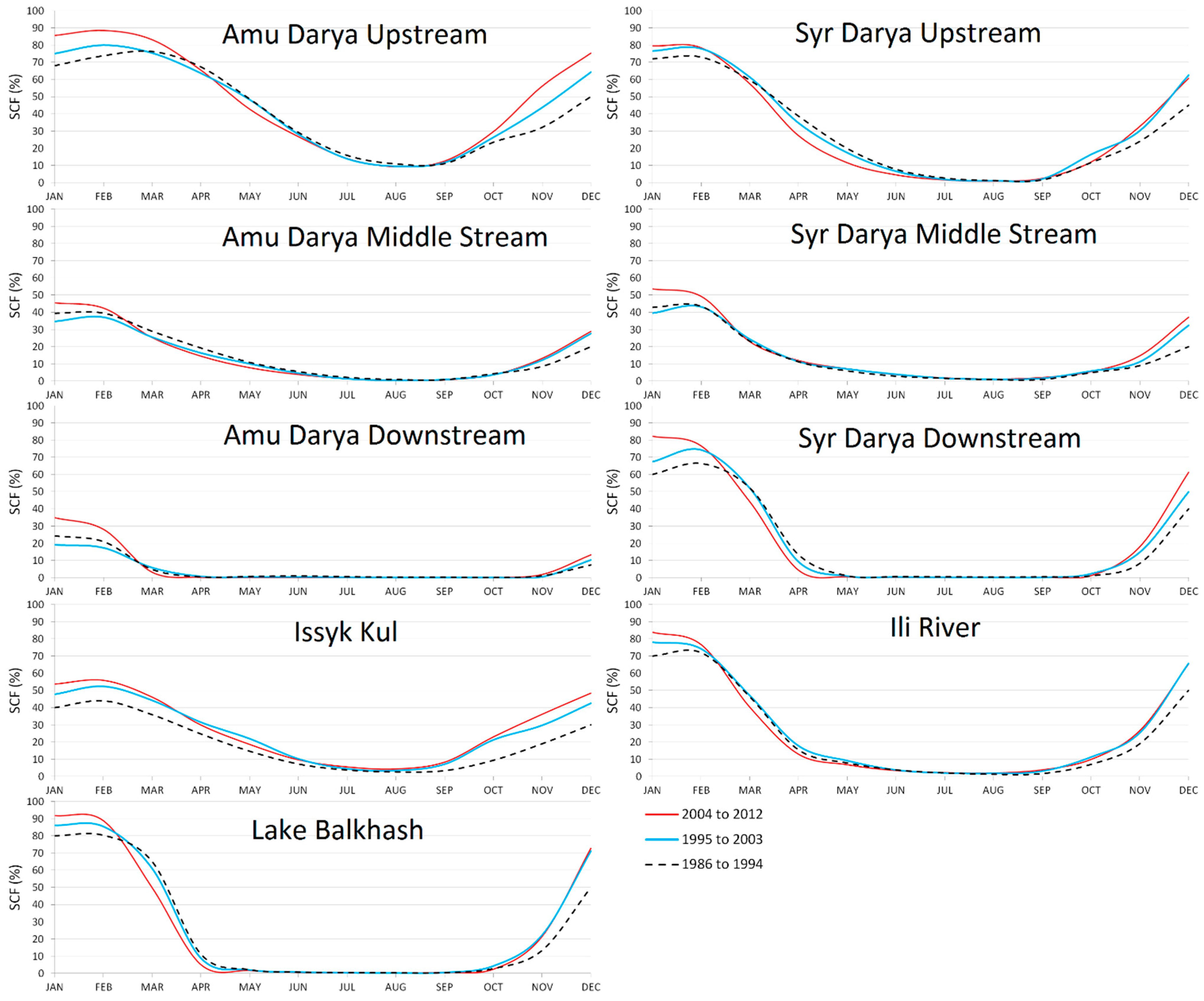
As the runoff in Central Asia’s rivers is highly snowmelt dominated [3,75,76] we are interested in the changes of snow cover within these river basins. The analysis of the time series of daily snow cover data for these catchments may help identifying possible long term changes of snow cover characteristics. For each group of subcatchments (upper, middle, and downstream) we aggregate the snow cover and calculate the mean Snow Cover Fraction (SCF) within the subcatchment group. The mean SCF indicates the areal percentage of a catchment being covered by snow at a certain time. To highlight the long term changes of snow cover characteristics within the catchment groups, we aggregate the mean SCF not only by month, but also for several years, and compare eight-year long periods against each other. The result of this analysis is illustrated in Figure 9. For each group of subcatchments, a diagram is included that shows the mean SCF for each month for three different eight-year periods: 1986 to 1994, 1995 to 2003, and 2004 to 2012. 2013 is not depicted in Figure 9. Years 1994 and 1999 stood out due to insuperable data gaps and have also been excluded from the calculations of the mean SCF results.

The plots in Figure 9 help to illustrate several snow-cover characteristics: First of all, the SCF magnitude describes the mean snow cover percentage of the whole catchment group per month. Some plots differ between the three time periods, giving a hint whether snow cover characteristics changed over time. Important information included in Figure 9 is those points where the plots from different periods converge or even cross each other’s path: Here, the speed of snow cover depletion or aggregation differs between the time periods. The steepness of the curves is the third valuable information: it indicates how fast snow cover aggregation and snow cover melt occur (though especially the latter is of interest for hydrological analyses).

Figure 9. Mean Snow Cover Fraction (SCF) for eight-year periods between 1986 and 2012 for Upstream, Middle Stream, and Downstream catchments of Amu Darya, Syr Darya, and Lake Balkhash catchment areas.

Figure 9. Mean Snow Cover Fraction (SCF) for eight-year periods between 1986 and 2012 for Upstream, Middle Stream, and Downstream catchments of Amu Darya, Syr Darya, and Lake Balkhash catchment areas.

A statistical trend of SCD, SCD_ES or SCD_LS cannot be identified from Figure 9 without further analyses, though some of the diagrams already give a superficial idea of the possible result. We conducted Mann-Kendall tests on the time series of snow cover data. The same tests were applied in a similar study for the Amu Darya River basin [15]. We decided to apply the same analysis in order to make the results from both studies comparable. Table 5 displays the slope (days per year) of SCD, SCD_ES or SCD_LS as derived from the time series of 28 successive years (again 1994 and 1999 were excluded from the time series and treated as missing values). Significant trends are indicated by bold letters while italic show non-significant slopes. The catchment groups are again the same as in Figure 8.

The trends from Table 5 can cover a wide range of different elevation zones. Some of the catchments (especially middle and upstream) cover altitude ranges from thousand meters and more. Because snow cover occurrence is highly dependent on elevation [67,77,78] and climate change affects higher mountain ranges more severely [79,80] it is important to analyze snow cover changes within different elevation zones. We used a DEM to extract possible trends in SCD_ES and SCD_LS for every 100 m zone within Central Asia. Table 6 contains the results of this DEM analysis, again for the full time series of 28 hydrological years between 1986/1987 and 2013/2014. This table also includes the land percentage covered by each of the elevation zones (in the share field) to give a better impression of how prominently a zone is represented among the whole study area.

Table 5. Trend of SCD_ES and SCD_LS per catchment group between 1986/1987 and 2013/2014.

Catchment	SCDES Slope *	SCDLS Slope *	SCD Slope *
Amu Darya Upstream	0.57	−0.40	0.44
Amu Darya Middle Stream	0.22	−0.32	0.03
Amu Darya Downstream	0.25	0.17	0.49
Syr Darya Upstream	0.58	−0.36	0.36
Syr Darya Middle Stream	0.40	−0.41	−0.04
Syr Darya Downstream	0.75	0.03	0.98
Issyk Kul	0.72	−0.27	0.73
Ili River	0.73	−0.30	0.22
Lake Balkhash	0.99	−0.06	1.09

* A bold slope indicates a trend detected under a significant level of 0.05; an italic slope represents a non-significant trend.

Table 5. Trend of SCD_ES and SCD_LS per catchment group between 1986/1987 and 2013/2014.

Catchment	SCDES Slope *	SCDLS Slope *	SCD Slope *
Amu Darya Upstream	0.57	−0.40	0.44
Amu Darya Middle Stream	0.22	−0.32	0.03
Amu Darya Downstream	0.25	0.17	0.49
Syr Darya Upstream	0.58	−0.36	0.36
Syr Darya Middle Stream	0.40	−0.41	−0.04
Syr Darya Downstream	0.75	0.03	0.98
Issyk Kul	0.72	−0.27	0.73
Ili River	0.73	−0.30	0.22
Lake Balkhash	0.99	−0.06	1.09

* A bold slope indicates a trend detected under a significant level of 0.05; an italic slope represents a non-significant trend.

Table 6. Trend of SCDES and SCDLS per elevation level between 1986/1987 and 2013/2014.

Elevation	SCDES Slope *	SCDLS Slope *	Share **	Elevation	SCDES Slope *	SCDLS Slope *	Share **
0–100 m	0.76	0.43	14.99	3501–3600 m	1.10	−0.32	0.28
101–200 m	1.28	0.51	23.56	3601–3700 m	1.15	−0.26	0.26
201–300 m	1.46	0.53	15.50	3701–3800 m	1.23	−0.24	0.25
301–400 m	1.63	0.54	9.62	3801–3900 m	1.33	−0.06	0.24
401–500 m	1.38	0.54	9.56	3901–4000 m	1.32	−0.10	0.23
501–600 m	1.42	0.49	4.79	4001–4100 m	1.26	−0.03	0.21
601–700 m	1.34	0.42	3.59	4101–4200 m	1.06	−0.16	0.20
701–800 m	1.26	0.33	2.61	4201–4300 m	1.07	−0.06	0.18
801–900 m	1.34	0.34	1.84	4301–4400 m	1.12	−0.04	0.16
901–1000 m	1.34	0.36	1.19	4401–4500 m	1.19	0.01	0.14
1001–1100 m	1.27	0.43	0.78	4501–4600 m	1.23	0.05	0.13
1101–1200 m	1.21	0.53	0.57	4601–4700 m	1.28	0.09	0.11
1201–1300 m	1.14	0.47	0.46	4701–4800 m	1.40	0.15	0.09
1301–1400 m	1.10	0.46	0.40	4801–4900 m	1.37	0.16	0.08
1401–1500 m	1.08	0.42	0.37	4901–5000 m	1.38	0.28	0.07
1501–1600 m	1.02	0.34	0.33	5001–5100 m	1.48	0.41	0.05
1601–1700 m	1.21	0.36	0.37	5101–5200 m	1.62	0.54	0.04
1701–1800 m	1.16	0.30	0.34	5201–5300 m	1.58	0.57	0.03
1801–1900 m	1.02	0.18	0.35	5301–5400 m	1.59	0.62	0.02
1901–2000 m	0.97	0.13	0.34	5401–5500 m	1.58	0.58	0.01
2001–2100 m	0.90	0.01	0.32	5501–5600 m	1.52	0.67	0.01
2101–2200 m	0.83	−0.04	0.30	5601–5700 m	1.52	0.66	0.00
2201–2300 m	0.80	−0.12	0.28	5701–5800 m	1.18	0.81	0.00
2301–2400 m	0.80	−0.15	0.27	5801–5900 m	1.16	0.76	0.00
2401–2500 m	0.78	−0.21	0.26	5901–6000 m	1.07	0.83	0.00
2501–2600 m	0.75	−0.22	0.26	6001–6100 m	0.85	0.69	0.00
2601–2700 m	0.75	−0.27	0.25	6101–6200 m	0.56	0.55	0.00
2701–2800 m	0.75	−0.31	0.25	6201–6300 m	0.67	0.72	0.00
2801–2900 m	0.72	−0.36	0.24	6301–6400 m	0.34	0.72	0.00
2901–3000 m	0.76	−0.40	0.25	6401–6500 m	0.55	0.82	0.00
3001–3100 m	0.81	−0.38	0.26	6501–6600 m	0.43	0.68	0.00
3101– 3200 m	0.87	−0.38	0.28	6601–6700 m	0.62	0.60	0.00
3201–3300 m	0.87	−0.38	0.28	6701–6800 m	0.22	0.33	0.00
3301–3400 m	0.96	−0.35	0.28	6801–6900 m	1.56	0.20	0.00
3401–3500 m	0.99	−0.32	0.27

^* A bold slope indicates a trend detected under a significant level of 0.05; an italic slope represents a non-significant trend; ^** Share refers to the percentage of an elevation range with regards to the total area of Central Asia. It indicates how much of the study region is represented by this elevation range.

Table 6. Trend of SCDES and SCDLS per elevation level between 1986/1987 and 2013/2014.

Elevation	SCDES Slope *	SCDLS Slope *	Share **	Elevation	SCDES Slope *	SCDLS Slope *	Share **
0–100 m	0.76	0.43	14.99	3501–3600 m	1.10	−0.32	0.28
101–200 m	1.28	0.51	23.56	3601–3700 m	1.15	−0.26	0.26
201–300 m	1.46	0.53	15.50	3701–3800 m	1.23	−0.24	0.25
301–400 m	1.63	0.54	9.62	3801–3900 m	1.33	−0.06	0.24
401–500 m	1.38	0.54	9.56	3901–4000 m	1.32	−0.10	0.23
501–600 m	1.42	0.49	4.79	4001–4100 m	1.26	−0.03	0.21
601–700 m	1.34	0.42	3.59	4101–4200 m	1.06	−0.16	0.20
701–800 m	1.26	0.33	2.61	4201–4300 m	1.07	−0.06	0.18
801–900 m	1.34	0.34	1.84	4301–4400 m	1.12	−0.04	0.16
901–1000 m	1.34	0.36	1.19	4401–4500 m	1.19	0.01	0.14
1001–1100 m	1.27	0.43	0.78	4501–4600 m	1.23	0.05	0.13
1101–1200 m	1.21	0.53	0.57	4601–4700 m	1.28	0.09	0.11
1201–1300 m	1.14	0.47	0.46	4701–4800 m	1.40	0.15	0.09
1301–1400 m	1.10	0.46	0.40	4801–4900 m	1.37	0.16	0.08
1401–1500 m	1.08	0.42	0.37	4901–5000 m	1.38	0.28	0.07
1501–1600 m	1.02	0.34	0.33	5001–5100 m	1.48	0.41	0.05
1601–1700 m	1.21	0.36	0.37	5101–5200 m	1.62	0.54	0.04
1701–1800 m	1.16	0.30	0.34	5201–5300 m	1.58	0.57	0.03
1801–1900 m	1.02	0.18	0.35	5301–5400 m	1.59	0.62	0.02
1901–2000 m	0.97	0.13	0.34	5401–5500 m	1.58	0.58	0.01
2001–2100 m	0.90	0.01	0.32	5501–5600 m	1.52	0.67	0.01
2101–2200 m	0.83	−0.04	0.30	5601–5700 m	1.52	0.66	0.00
2201–2300 m	0.80	−0.12	0.28	5701–5800 m	1.18	0.81	0.00
2301–2400 m	0.80	−0.15	0.27	5801–5900 m	1.16	0.76	0.00
2401–2500 m	0.78	−0.21	0.26	5901–6000 m	1.07	0.83	0.00
2501–2600 m	0.75	−0.22	0.26	6001–6100 m	0.85	0.69	0.00
2601–2700 m	0.75	−0.27	0.25	6101–6200 m	0.56	0.55	0.00
2701–2800 m	0.75	−0.31	0.25	6201–6300 m	0.67	0.72	0.00
2801–2900 m	0.72	−0.36	0.24	6301–6400 m	0.34	0.72	0.00
2901–3000 m	0.76	−0.40	0.25	6401–6500 m	0.55	0.82	0.00
3001–3100 m	0.81	−0.38	0.26	6501–6600 m	0.43	0.68	0.00
3101– 3200 m	0.87	−0.38	0.28	6601–6700 m	0.62	0.60	0.00
3201–3300 m	0.87	−0.38	0.28	6701–6800 m	0.22	0.33	0.00
3301–3400 m	0.96	−0.35	0.28	6801–6900 m	1.56	0.20	0.00
3401–3500 m	0.99	−0.32	0.27

^* A bold slope indicates a trend detected under a significant level of 0.05; an italic slope represents a non-significant trend; ^** Share refers to the percentage of an elevation range with regards to the total area of Central Asia. It indicates how much of the study region is represented by this elevation range.

5. Discussions

The study of changing snow cover characteristics produced a large set of results. Twenty-eight years of SCD, SCD_ES and SCD_LS have been processed from more than 20,000 raw AVHRR scenes and around 76,000 MODIS snow cover product datasets. The processed area comprises 4 Mio km², which, combined with the long time series of medium resolution remote sensing data, causes a huge amount of data. We tried to select and present only those of utmost interest for the scientific community which turned out to be a difficult task given the broad spectrum of possible applications/analyses that become possible from a time series of snow cover data—as already outlined in Section 1. The presented results (Figure 8 and Figure 9; Table 5 and Table 6) describe basically three findings:

• The general characteristics of SCD within Central Asia. Figure 8 depicts the mean SCD between 2000/2001 and 2013/2014 for the main catchments areas (Figure 8 (a–c)) as well as for the whole area of Central Asia (Figure 8d). SCD increases by around four days per 100 m elevation. The mountainous regions in the south and southeast contain the highest values of SCD. The glaciers of Central Asia are located in this region too. It is the origin of the most significant rivers of Central Asia: Amu Darya, Syr Darya, and Ili River. In the plains, SCD increases by around 5 days per degree latitude until mean SCD reaches 140 in the most northern parts (at around 54° N). Figure 8 (a–d) describe the SCD as it can be expected today. However; the variability within the time series is huge (which is not shown here but for example in [14]). Every year reveals its own peculiarities but the results behind Figure 8 can be used to analyze and compare every upcoming snow cover season against these mean conditions to identify abnormal conditions.
• The diagrams in Figure 9 and the statistics from Table 5 describe an important change in snow cover characteristics since 1986: The snow cover season is shifting towards an earlier time. The slope of SCD_ES is positive for all catchment groups, meaning that the snow cover season is generally starting earlier today than in the late 1980s. Except for Amu Darya Middle stream, all of the presented trends are significant. SCD_LS on the other hand is affected by a negative slope for most catchment groups except two, which are located downstream. The significance of these slopes is not as distinct as it is for the early season, but the most essential catchments in the upstream region show a significant level of 0.05. This is an important finding as most of Central Asia’s runoff is generated within these upstream catchments and a shift towards earlier snow cover onset and melt can influence the water availability of the whole region considerably.
• The results presented in Table 6 are segmented according to elevation levels of 100 m and show another very important finding about snow cover changes in Central Asia: The slope of SCD_ES is positive for all elevation zones regardless of their altitude while most of these trends are significant. In other words: Snow cover is starting earlier every year since 1986 throughout all elevation ranges. The slopes of SCD_LS on the other hand are two-sided: Below 1800 m, the trend is significantly positive, describing a prolonged snow cover season with later snow cover melts. Between an altitude of 1800 and 2500 m the situation can best be interpreted as a transition zone: The positive trend is still present at the beginning but it is not significant anymore. With increasing altitude, the trend switches to a negative but not yet significant value. Only above 2500 m, the slope of SCD_LS becomes significantly negative. In this region, snow cover melt occurs earlier today than in the late 1980s and can be expected to continue developing in this direction also in the future. After the altitude reaches 3300 m, the negative trend is still present but not significant anymore as snow cover development is again entering a transition zone of unstable character. Above 5500 m, the trend is significantly positive again.

We have to consider two points when analyzing snow cover according to elevation for whole Central Asia: It is a vast area with 4 Mio km² so generalizing over elevation ranges also means generalizing over several degrees latitude and longitude, including different climatic regions as well. This is especially true for the lower altitudes, as most of Central Asia (~87%) is situated below 800 m elevation. Most of the hills and mountains situated above 800 m are located in the south and southeast and therefore, statistics from these regions are more significant. The second point is the aspect of the mountain sides: when averaging over elevation zones, both south and north facing slopes are aggregated to one single class. The difference between the northern side where solar insulation is comparably low, and the southern side with opposed insulation characteristics, can lead to a 2.8 times higher heat input on the southern side [78]. These differences are not considered within our analyses—partly because the 1 km resolution of the AVHRR data is not suited to derive sophisticated results on such regional scales.

When it comes to the interpretation of the presented results and the discussion of the possible long term consequences, the changes of SCD_ES and SCD_LS play a most significant role: The earlier SCD_ES can be observed through all elevation ranges and in all major catchment groups. The consequences for Central Asia’s water availability are marginal though, as the water is stored within the snowpack and released only after snowmelt. Therefore, changes in SCD_LS are much more important. The negative SCD_LS trend within major catchment groups of Amu Darya, Syr Darya, and Ili River is proof that Central Asia’s hydrology faces fundamental changes. The results extracted from optical remote sensing data are not suitable to state about snow depth (and therefore water content of a snowpack), but the fact that snowmelt is occurring up to eleven days earlier today than in 1986 (in case of Amu Darya and Syr Darya Upstream catchments for example) clearly emphasizes the significance of the findings.

The primary aim of the study—to analyze how snow cover has changed in Central Asia—has already been addressed to within the discussions above. The second aim—to compare the obtained results with a similar study about snow cover changes within Amu Darya catchment—is yet to be answered. Some of the conclusions drawn by [15] differ slightly from what we found during our investigations. A general negative trend of SCD that was identified by the authors of this study could not be confirmed for Central Asia. The trend towards earlier snow cover melts and for some areas earlier snow cover onset, however, coincides with what we analyzed from the snow cover time series. We interpret this as a clear confirmation of the fact that SCD_LS is shifting to earlier dates with each year.

6. Conclusions

We processed time series of medium resolution snow cover data for Central Asia between 1986 and 2014 to calculate the snow cover parameters Snow Cover Duration (SCD), Early Season SCD (SCD_ES) and Late Season SCD (SCD_LS)_, and analyze these parameters for possible trends. Around 20,000 AVHRR Level 1B scenes and 76,000 MODIS snow cover product MOD10A1 and MYD10A1 datasets were used as the basis of the study. The processing included preprocessing and snow cover classification of AVHRR data as well as post-processing of the AVHRR and MODIS snow cover products to estimate snow cover status below clouds. As a result, a positive trend of SCD_ES has been identified from the time series for all of Central Asia’s major hydrological catchments. SCD_LS on the other hand shows a different behavior: The upstream catchments show a significantly negative trend which is caused by fundamental negative snow cover changes in an elevation range between 2100 and 3500 m (significantly negative between 2500 and 3200 m). Though no distinct trend in overall SCD was identified, the shift towards earlier snow cover onset and earlier snow cover melt is proof for a changing cryosphere in Central Asia. Especially the trend of earlier SCD_LS could be confirmed also by comparing our results with an independent study for the Amu Darya River catchment. As the region greatly depends on snow as the most prominent source of freshwater the identified changes point to an ambiguous future: the Aral Sea Disaster, population growth, increasing energy demands, transboundary water issues—these are just few examples for the challenges Central Asia faces right now [10,81,82,83]. Further analyses are required to assess the possible impact of the identified snow cover changes with regards to all these problems. As the analyzed trends will prolong into the future, techniques should be developed and applied in order to mitigate their effects.

A final remark is necessary referring to the reliability of the presented trend results: Significance has been tested computing the Kendall’s S statistics and deriving Kendall’s tau correlation coefficient to test whether the null hypothesis is true or can be rejected. Those trend results that proved significant according to this test have been marked with bold letters in the respective tables as described in Section 4. However: Deriving trends over such short time series is a risky endeavor. Unfortunately it was not possible to compute additional robustness tests, which would be desirable to substantiate our findings. Therefore, the presented results should be interpreted with care.

References

1. Klein, I.; Gessner, U.; Kuenzer, C. Regional land cover mapping and change detection in Central Asia using MODIS time-series. Appl. Geogr. 2012, 35, 219–234. [Google Scholar] [CrossRef]
2. Aizen, V.B.; Aizen, E.M.; Melack, J.M. Climate, snow cover, glaciers, and runoff in the Tien Shan, Central Asia. Water Resour. Bull. 1995, 31, 1113–1129. [Google Scholar] [CrossRef]
3. Ososkova, T.; Gorelkin, N.; Chub, V. Water resources of Central Asia and adaptation measures for climate change. Environ. Monit. Assess. 2000, 61, 161–166. [Google Scholar] [CrossRef]
4. Lioubimtseva, E.; Henebry, G.M. Climate and environmental change in arid Central Asia: Impacts, vulnerability, and adaptations. J. Arid Environ. 2009, 73, 963–977. [Google Scholar] [CrossRef]
5. Aizen, V.B.; Kuzmichenok, V.A.; Surazakov, A.B.; Aizen, E.M. Glacier changes in the central and northern Tien Shan during the last 140 years based on surface and remote-sensing data. Ann. Glaciol. 2006, 43, 202–213. [Google Scholar] [CrossRef]
6. Micklin, P. The aral sea disaster. Ann. Rev. Earth Planet. Sci. 2007, 35, 47–72. [Google Scholar] [CrossRef]
7. Strickman, R.; Porkka, M. Water and Social Changes in Central Asia: Problems Related to Cotton Production in Uzbekistan. Available online: http://water.tkk.fi/English/wr/research/global/material/Central_Asian_Waters-book.pdf#page=113 (accessed on 10 October 2014).
8. Bernauer, T.; Siegfried, T. Climate change and international water conflict in Central Asia. J. Peace Res. 2012, 49, 227–239. [Google Scholar] [CrossRef]
9. Aizen, V.B.; Aizen, E.M.; Melack, J.; Dozier, J. Climatic and hydrologic changes in the Tien Shan, Central Asia. J. Clim. 1997, 10, 1393–1404. [Google Scholar] [CrossRef]
10. Siegfried, T.; Bernauer, T.; Guiennet, R.; Sellars, S.; Robertson, A.W.; Mankin, J.; Bauer-Gottwein, P.; Yakovlev, A. Will climate change exacerbate water stress in Central Asia? Clim. Change 2011, 112, 881–899. [Google Scholar] [CrossRef]
11. Rakhmatullaev, S.; Huneau, F.; Le Coustumer, P.; Motelica-Heino, M.; Bakiev, M. Facts and perspectives of water reservoirs in Central Asia: A special focus on Uzbekistan. Water 2010, 2, 307–320. [Google Scholar] [CrossRef]
12. Glantz, M.H. Water, climate, and development issues in the Amu Darya Basin. Mitig. Adapt. Strat. Glob. Change 2005, 10, 23–50. [Google Scholar] [CrossRef]
13. Granit, J.; Jägerskog, A.; Löfgren, R.; Bullock, A.; Gooijer, G. De; Pettigrew, S.; Lindström, A. Regional Water Intelligence Report Central Asia. Available online: http://www.watergovernance.org/documents/WGF/Reports/Paper-15_RWIR_Aral_Sea.pdf (accessed on 10 October 2014).
14. Dietz, A.J.; Kuenzer, C.; Conrad, C. Snow-cover variability in central Asia between 2000 and 2011 derived from improved MODIS daily snow-cover products. Int. J. Remote Sens. 2013, 34, 3879–3902. [Google Scholar] [CrossRef]
15. Zhou, H.; Aizen, E.; Aizen, V. Deriving long term snow cover extent dataset from AVHRR and MODIS data: Central Asia case study. Remote Sens. Environ. 2013, 136, 146–162. [Google Scholar] [CrossRef]
16. International Monetary Fund. Available online: http://www.imf.org/external/ (accessed on 14 July 2014).
17. Lucas, R.M.; Harrison, A.R. Snow observation by satellite: A review. Remote Sens. Rev. 1990, 4, 285–348. [Google Scholar] [CrossRef]
18. Dietz, A.J.; Kuenzer, C.; Gessner, U.; Dech, S. Remote sensing of snow—A review of available methods. Int. J. Remote Sens. 2012, 13, 4094–4134. [Google Scholar] [CrossRef]
19. Solberg, R.; Koren, H.; Amlien, J. A Review of Optical Snow Cover Algorithms. Available online: http://www.nr.no/en/nrpublication?query=/file/4400/Solberg_-_A_review_of_optical_snow_algorithms.pdf (accessed on 10 October 2014).
20. Frei, A.; Tedesco, M.; Lee, S.; Foster, J.; Hall, D.K.; Kelly, R.; Robinson, D.A. A review of global satellite-derived snow products. Adv. Space Res. 2012, 50, 1007–1029. [Google Scholar] [CrossRef]
21. König, M.; Winther, J.; Isaksson, E. Measuring snow and glacier ice properties from satellite. Rev. Geophys. 2001, 39, 1–27. [Google Scholar] [CrossRef]
22. WMO. GCOS Systematic Observation Requirements for Satellite-Based Data Products for Climate-2011 Update; WMO GCOS: Geneva, Switzerland, 2011; p. 127. [Google Scholar]
23. Klein, A.G.; Hall, D.K.; Nolin, A.W. Development of a prototype snow albedo algorithm for the NASA MODIS Instrument. In Proceedings of 57th Eastern Snow Conference, Syracuse, NY, USA, 2–3 June 2000; pp. 143–158.
24. Khlopenkov, K.V.; Trishchenko, A.P. SPARC: New cloud, snow, and cloud shadow detection scheme for historical 1-km AVHHR data over Canada. J. Atmos. Ocean. Technol. 2007, 24, 322–343. [Google Scholar] [CrossRef]
25. Hüsler, F.; Jonas, T.; Wunderle, S.; Albrecht, S. Validation of a modified snow cover retrieval algorithm from historical 1-km AVHRR data over the European Alps. Remote Sens. Environ. 2012, 121, 497–515. [Google Scholar] [CrossRef]
26. Wang, L.; Derksen, C.; Brown, R. Detection of pan-Arctic terrestrial snowmelt from QuikSCAT, 2000–2005. Remote Sens. Environ. 2008, 112, 3794–3805. [Google Scholar] [CrossRef]
27. Rott, H.; Künzi, K.F. Remote sensing of snow cover with passive and active microwave sensors. Hydrol. Appl. Remote Sens. Data Trans. 1983, 145, 361–369. [Google Scholar]
28. Song, K.; Zhang, Y. Snow-cover environmental monitoring and assessment in Northeast China using passive microwave emission models. Environ. Monit. Assess. 2008, 140, 223–9. [Google Scholar] [CrossRef] [PubMed]
29. Derksen, C. The contribution of AMSR-E 18.7 and 10.7 GHz measurements to improved boreal forest snow water equivalent retrievals. Remote Sens. Environ. 2008, 112, 2701–2710. [Google Scholar] [CrossRef]
30. Tedesco, M.; Miller, J. Northern hemisphere snow-covered area mapping: Optical versus active and passive microwave data. IEEE Geosci. Remote Sens. Lett. 2007, 4, 221–225. [Google Scholar] [CrossRef]
31. Amlien, J. Remote Sensing of Snow with Passive Microwave Radiometers—A Review of Current Algorithms. Available online: http://www.nr.no/en/nrpublication?query=/file/4936/Amlien_-_Remote_sensing_of_snow_with_passive_microwave_radi.pdf (accessed on 10 October 2014).
32. Luojus, K.P.; Pulliainen, J.T.; Takala, M.; Kangwa, M.; Smolander, T. GlobSnow-2 Product User Guide; Finnish Meteorological Institute: Helsinki, Finland, 2013; pp. 0–23. [Google Scholar]
33. Donlon, C.; Berruti, B.; Buongiorno, A.; Ferreira, M.-H.; Féménias, P.; Frerick, J.; Goryl, P.; Klein, U.; Laur, H.; Mavrocordatos, C.; et al. The global monitoring for environment and security (GMES) sentinel-3 mission. Remote Sens. Environ. 2012, 120, 37–57. [Google Scholar] [CrossRef]
34. Dozier, J. Spectral signature of alpine snow cover from the Landsat Thematic Mapper. Remote Sens. Environ. 1989, 28, 9–22. [Google Scholar] [CrossRef]
35. Drusch, M.; Del Bello, U.; Carlier, S.; Colin, O.; Fernandez, V.; Gascon, F.; Hoersch, B.; Isola, C.; Laberinti, P.; Martimort, P.; et al. Sentinel-2: ESA’s optical high-resolution mission for GMES operational services. Remote Sens. Environ. 2012, 120, 25–36. [Google Scholar] [CrossRef]
36. ESA. ATSR Mission Description. Available online: https://earth.esa.int/web/guest/missions/esa-operational-eo-missions/ers/instruments/atsr (accessed on 1 October 2014).
37. ESA. AATSR Mission Description. Available online: https://earth.esa.int/web/guest/missions/esa-operational-eo-missions/envisat/instruments/aatsr (accessed on 1 October 2014).
38. Hall, D.K.; Riggs, G.A.; Salomonson, V.V. Development of methods for mapping global snow cover using moderate resolution imaging spectroradiometer data. Remote Sens. Environ. 1995, 54, 127–140. [Google Scholar] [CrossRef]
39. Malenovský, Z.; Rott, H.; Cihlar, J.; Schaepman, M.E.; García-Santos, G.; Fernandes, R.; Berger, M. Sentinels for science: Potential of Sentinel-1, -2, and -3 missions for scientific observations of ocean, cryosphere, and land. Remote Sens. Environ. 2012, 120, 91–101. [Google Scholar] [CrossRef]
40. Solberg, R.; Wangensteen, B.; Amlien, J.; Koren, H.; Metsämäki, S.; Nagler, T.; Luojus, K.; Pulliainen, J. A new global snow extent product based on ATSR-2 and AATSR. In Proceedings of the 2010 IEEE International Geoscience and Remote Sensing Symposium, Honolulu, HI, USA, 25–30 July 2010.
41. Rosenfeld, D.; Liu, G.; Yu, X.; Zhu, Y.; Dai, J.; Xu, X.; Yue, Z. High-resolution (375 m) cloud microstructure as seen from the NPP/VIIRS satellite imager. Atmos. Chem. Phys. 2014, 14, 2479–2496. [Google Scholar] [CrossRef]
42. NOAA’s Comprehensive Large Array-Data Stewardship System. Available online: http://www.class.noaa.gov (accessed on 3 November 2014).
43. Gesell, G. An algorithm for snow and ice detection using AVHRR data: An extension to the APOLLO software package. Int. J. Remote Sens. 1989, 10, 897–905. [Google Scholar] [CrossRef]
44. Saunders, R.W.; Kriebel, K.T. An improved method for detecting clear sky and cloudy radiances from AVHRR data. Int. J. Remote Sens. 1988, 9, 123–150. [Google Scholar] [CrossRef]
45. NOAA/NESDIS. NOAA KLM User’s Guide with NOAA-N, -P Supplement. Available online: http://www.ncdc.noaa.gov/oa/pod-guide/ncdc/docs/klm/index.htm (accessed on 23 July 2012).
46. NOAA/NESDIS. NOAA Polar Orbiter Data User’s Guide. Available online: http://www.ncdc.noaa.gov/oa/pod-guide/ncdc/docs/podug/index.htm (accessed on 22 July 2012).
47. Hall, D.K.; Riggs, G.A.; Salomonson, V.V. MODIS/Terra Snow Cover Daily L3 Global 500m Grid, Version 5. Available online: https://nsidc.org/data/docs/daac/modis_v5/mod10a1_modis_terra_snow_daily_global_500m_grid.gd.html (accessed on 10 October 2014).
48. Crane, R.G.; Anderson, M.R. Satellite discrimination of snow/cloud surfaces. Int. J. Remote Sens. 1984, 5, 213–223. [Google Scholar] [CrossRef]
49. Salomonson, V.V.; Appel, I. Development of the Aqua MODIS NDSI fractional snow cover algorithm and validation results. IEEE Trans. Geosci. Remote Sens. 2006, 44, 1747–1756. [Google Scholar] [CrossRef]
50. Klein, A.G.; Barnett, A.C. Validation of daily MODIS snow cover maps of the Upper Rio Grande River Basin for the 2000–2001 snow year. Remote Sens. Environ. 2003, 86, 162–176. [Google Scholar] [CrossRef]
51. Painter, T.H.; Rittger, K.; McKenzie, C.; Slaughter, P.; Davis, R.E.; Dozier, J. Retrieval of subpixel snow covered area, grain size, and albedo from MODIS. Remote Sens. Environ. 2009, 113, 868–879. [Google Scholar] [CrossRef]
52. Hall, D.; Riggs, G. Accuracy assessment of the MODIS snow products. Hydrol. Process. 2007, 21, 1534–1547. [Google Scholar] [CrossRef]
53. Maurer, E.P.; Rhoads, J.D.; Dubayah, R.O.; Lettenmaier, D.P. Evaluation of the snow-covered area data product from MODIS. Hydrol. Process. 2003, 17, 59–71. [Google Scholar] [CrossRef]
54. Parajka, J.; Blöschl, G. Validation of MODIS snow cover images over Austria. Hydrol. Earth Syst. Sci. 2006, 10, 679–689. [Google Scholar] [CrossRef]
55. Huang, X.; Liang, T.; Zhang, X.; Guo, Z. Validation of MODIS snow cover products using Landsat and ground measurements during the 2001–2005 snow seasons over northern Xinjiang, China. Int. J. Remote Sens. 2011, 32, 133–152. [Google Scholar] [CrossRef]
56. Simic, A.; Fernandes, R.; Brown, R.; Romanov, P.; Park, W. Validation of VEGETATION, MODIS, and GOES+ SSM/I snow-cover products over Canada based on surface snow depth observations. Hydrol. Process. 2004, 18, 1089–1104. [Google Scholar] [CrossRef]
57. Wang, X.; Xie, H.; Liang, T. Evaluation of MODIS snow cover and cloud mask and its application in Northern Xinjiang, China. Remote Sens. Environ. 2008, 112, 1497–1513. [Google Scholar] [CrossRef]
58. Hall, D.K.; Foster, J.L.; Salomonson, V.V.; Klein, A.G.; Chien, J.Y.L. Development of a technique to assess snow-cover mapping errors from space. IEEE Trans. Geosci. Remote Sens. 2001, 39, 432–438. [Google Scholar] [CrossRef]
59. Bormann, K.J.; McCabe, M.F.; Evans, J.P. Satellite based observations for seasonal snow cover detection and characterisation in Australia. Remote Sens. Environ. 2012, 123, 57–71. [Google Scholar] [CrossRef]
60. Riggs, G.A.; Hall, D.K.; Salomonson, V.V. MODIS Snow Products User Guide to Collection 5; National Snow and Ice Data Center: Boulder, CO, USA, 2006. [Google Scholar]
61. Stowe, L.L.; Davis, P.A.; McClain, P.E. Scientific basis and initial evaluation of the CLAVR-1 global clear/cloud classification algorithm for the advanced very high resolution radiometer. J. Atmos. Ocean. Technol. 1998, 16, 656–681. [Google Scholar] [CrossRef]
62. Dech, S.W.; Tungalagsaikhan, P.; Preusser, C.; Meisner, R.E. Operational value-adding to AVHRR data over Europe: Methods, results, and prospects. Aerosp. Sci. Technol. 1998, 2, 335–346. [Google Scholar] [CrossRef]
63. Kriebel, K.T.; Gesell, G.; Kästner, M.; Mannstein, H. The cloud analysis tool APOLLO: improvements and validations. Int. J. Remote Sens. 2003, 24, 2389–2408. [Google Scholar] [CrossRef]
64. TeraScan Software Package. Available online: http://www.seaspace.com/software.php (accessed on 17 December 2014).
65. Gafurov, A.; Bárdossy, A. Cloud removal methodology from MODIS snow cover product. Hydrol. Earth Syst. Sci. 2009, 13, 1361–1373. [Google Scholar] [CrossRef]
66. Jarvis, A.; Reuter, H.I.; Nelson, A.; Guevara, E. Hole-filled SRTM for the Globe Version 4. Available online: http://srtm.csi.cgiar.org (accessed on 10 October 2014).
67. Parajka, J.; Pepe, M.; Rampini, A.; Rossi, S.; Blöschl, G. A regional snow-line method for estimating snow cover from MODIS during cloud cover. J. Hydrol. 2010, 381, 203–212. [Google Scholar] [CrossRef]
68. Dietz, A.J.; Wohner, C.; Kuenzer, C. European snow cover characteristics between 2000 and 2011 derived from improved MODIS daily snow cover products. Remote Sens. 2012, 4, 2432–2454. [Google Scholar] [CrossRef]
69. Wang, X.; Xie, H. New methods for studying the spatiotemporal variation of snow cover based on combination products of MODIS Terra and Aqua. J. Hydrol. 2009, 371, 192–200. [Google Scholar] [CrossRef]
70. Brown, R.; Derksen, C.; Wang, L. Assessment of spring snow cover duration variability over Northern Canada from satellite datasets. Remote Sens. Environ. 2007, 111, 367–381. [Google Scholar] [CrossRef]
71. Hantel, M.; Ehrendorfer, M.; Haslinger, A. Climate sensitivity of snow cover duration in Austria. Int. J. Climatol. 2000, 20, 615–640. [Google Scholar] [CrossRef]
72. Falarz, M. Variability and trends in the duration and depth of snow cover in Poland in the 20th century. Int. J. Climatol. 2004, 24, 1713–1727. [Google Scholar] [CrossRef]
73. Brown, R.D.; Mote, P.W. The response of Northern Hemisphere snow cover to a changing climate. J. Clim. 2009, 22, 2124–2145. [Google Scholar] [CrossRef]
74. Armstrong, R. Historical Soviet Daily Snow Depth Version 2. Available online: http://nsidc.org/data/docs/noaa/g01092_hsdsd/index.html (accessed on 10 October 2014).
75. Barnett, T.P.; Adam, J.C.; Lettenmaier, D.P. Potential impacts of a warming climate on water availability in snow-dominated regions. Nature 2005, 438, 303–309. [Google Scholar] [CrossRef] [PubMed]
76. Adam, J.C.; Hamlet, A.F.; Lettenmaier, D.P. Implications of global climate change for snowmelt hydrology in the twenty-first century. Hydrol. Process. 2009, 23, 962–972. [Google Scholar] [CrossRef]
77. Severskiy, I.V. Distribution of Snow Cover in the Mountains of Central Asia. Available online: http://lib.icimod.org/record/24560/files/c_attachment_347_5309.pdf (accessed on 10 October 2014).
78. Severskiy, I.V.; Blagoveshchenskiy, V.P.; Severskiy, S.I.; Pimankina, N.V.; Zichu, X.; Zhizhong, Z.; Ruji, H. Influence of local factors on the distribution of snow cover in mountains. In Snow Cover and Avalanches in Tien Shan Mountains; Severskiy, I.V., Zichu, X., Eds.; VAC Publishing House: Almaty, Kazakhstan, 2000; pp. 91–106. [Google Scholar]
79. Beniston, M. Climatic change in mountain regions: A review of possible impacts. Clim. Change 2003, 36, 281–300. [Google Scholar] [CrossRef]
80. Räisänen, J.; Eklund, J. 21st Century changes in snow climate in Northern Europe: A high-resolution view from ENSEMBLES regional climate models. Clim. Dynam. 2012, 38, 2575–2591. [Google Scholar] [CrossRef]
81. Diebold, A.; Sehring, J. From the Glaciers to the Aral Sea-Water Unites, 1st ed.; Trescher Verlag: Berlin, Germany, 2012. [Google Scholar]
82. Jalilov, S.; Desutter, T.M.; Leitch, J.A. Impact of Rogun dam on downstream Uzbekistan agriculture. Int. J. Water Resour. Environ. Eng. 2011, 3, 161–166. [Google Scholar]
83. Lillis, J. Uzbekistan Leader Warns of Water Wars in Central Asia. Available online: http://www.eurasianet.org/node/65877 (accessed on 7 September 2012).