Spatial Pattern and Temporal Variation Law-Based Multi-Sensor Collaboration Method for Improving Regional Soil Moisture Monitoring Capabilities

Abstract

Regional soil moisture distributions and changes are critical for agricultural production and environmental modeling. Currently, hundreds of satellite sensors exist with different soil moisture observation capabilities. However, multi-sensor collaborative observation mechanisms for improving regional soil moisture monitoring capabilities are lacking. In this study, a Spatial pattern and Temporal variation law-based Multi-sensor Collaboration (STMC) method is proposed to solve this problem. The first component of the STMC method deduces the regional soil moisture distribution and variation patterns based on time stability theory and long-term statistical analyses. The second component of the STMC method detects potential anomalous soil moisture events and immediately triggers the high spatial resolution sensor with the soonest pass-over time. In the detection phase, an anomalous soil moisture judgment (ASMJ) algorithm and high temporal resolution sensors (the Advanced Microwave Scanning Radiometer 2 (AMSR2)) were utilized. Experiments conducted in Hubei province, China, demonstrated that the proposed STMC method was capable of accurately identifying of anomalous soil moisture conditions caused by waterlogging and drought events. Additionally, we observed that the STMC method combined the advantages of different long-term observation, high temporal, and high spatial resolution sensors synergistically for monitoring purposes.

1. Introduction

Soil moisture plays an important role in the exchange of energy and materials between the atmosphere and the land surface [1,2,3]. Monitoring spatial and temporal changes in soil moisture is an attractive area of research [4,5,6]. However, due to the heterogeneity of the surface soil moisture [7], monitoring regional soil moisture in a timely and precise manner remains challenging [8]. So far, the capabilities of single remote sensing sensors for monitoring soil moisture have been widely investigated and proven [9,10,11,12,13,14].

Recently, more sensors have become available for soil moisture monitoring, including the Microwave Imaging Radiometer using Aperture Synthesis (MIRAS) [11], the Advanced Microwave Scanning Radiometer 2, and the Operational Land Imager sensors. According to the World Meteorological Organization, up to 120 satellite-based sensors are available for measuring the soil moisture of the surface around the world [15]. Therefore, the efficient use of these multiple sensors for enhancing regional soil moisture monitoring, such as quality or timeliness, is a promising area of research [16,17].

Mainstream research studies have explored the methods of combining, assimilating, and fusing multi-sensor data to promote monitoring capabilities [18]. These studies have taken advantage of data from different sensors to avoid the limited capabilities of the data from a single remote sensor [19]. For example, Prakash et al. [20] used the Phased Array type L-band Synthetic Aperture Radar (SAR) and the Moderate Resolution Imaging Spectroradiometer (MODIS) data by a new algorithm for soil moisture retrieval in vegetation-covered areas. Hosseini and Saradjian [21] showed that the integration of optical and SAR data (i.e., hybrid models) results in higher accuracy than single SAR models or optical models. In addition, fractal theory was also used for pattern recognition [22] and soil variation modeling [23]. Data from multiple sensors can provide more quantified parameters or information for physical models and semi-empirical inversion models. Thus, the Observed Data-based Multi-sensor Collaboration method (ODMC method) is capable of monitoring regional soil moisture [19,20,21].

However, if the monitoring is only based on this ODMC method, it is not sufficient for promoting the regional soil moisture monitoring capability to a higher level, because it only integrates multi-sensor data in terms of the electromagnetic spectrum. There still exists some room for improvement in terms of space and time.

With the wide acceptance of Sensor Web [24], earth observations have become more intelligent and high efficient [25,26]. Sensor Web is defined as a web of interconnected heterogeneous sensors that are interoperable, intelligent, dynamic, flexible, and scalable [27]. Thus, Sensor Web is a universe of network-accessible sensors, sensory data and information. By connecting all sensors in a universal network, the original isolated sensors become web-ready sensors. Thus, the data and information generated by the individual web-ready sensors are interoperable and the sensor services are chainable. Therefore, all sensors in this network can communicate and share information between each other, and the subsequent observations can be optimized accordingly [28]. This feature is important for realizing real-time Earth monitoring, which aims to detect potential emergencies more quickly than before. Actually, these new ideas in Sensor Web are one type of multi-sensor collaboration, because the sensors cooperate with each other to accomplish one mission [28].

This type of collaboration idea has proved advantages for monitoring forest fire [29,30,31] and flood disasters [32,33] during the last decade. In 2004 and 2006, NASA tested a multi-sensor collaboration method based on MODIS, in situ sensors, the Advanced Land Imager (ALI) and the Hyperion on EO-1 [29,30]. High-frequency MODIS measurements were used to locate terrestrial events, such as forest fires, and triggered high-resolution ALI or Hyperion sensors. In this experiment, EO-1 was driven by the low-resolution MODIS to ensure that the observations could be made in a timely manner and to obtain more focused images. In 2009, Liu et al. [31] proved that combining of MODIS and Formosat-2 based on optimization during the sensor planning stage could be used to rapidly locate fire points during wildfires. In 2013, the German Remote Sensing Data Center and German Aerospace Center proposed a MODIS and TerraSAR-X collaboration method to identify and monitor the evolution of floods at an early state. Time efficiency was achieved by using daily-acquired MODIS data to optimize the time-critical on-demand programming of the high-resolution SAR acquisitions for detailed flood monitoring [32]. In 2014, Lacava et al. [33] also demonstrated that the collaboration of MODIS and AMSR-E was helpful in a timely detection and a near real time monitoring of flood.

Regarding the soil moisture domain, to our knowledge, no method exists that adopts this type of collaboration method. This method attempts to use near real-time monitoring results from remote sensors to determine potential soil moisture emergencies and subsequently to optimize high-resolution sensors.

All existing collaboration methods used to monitor soil moisture are classified as the ODMC method, which utilizes observed data [18,19,20,21]. However, the promotion of monitoring capabilities during the observation stage based on new types of collaboration ideas from Sensor Web has not been explored yet. In addition, it is more difficult to monitor soil moisture changes than to monitor forest fires or floods because soil moisture changes occur daily and anomalous events are difficult to define [34]. However, when forest fires and floods occur, their distinguishing features can be detected easily [29,30,31,32,33]. Therefore, it is challenging to monitor soil moisture collaboratively.

In this study, we aim to explore new monitoring capabilities in the sensor observation (also called scheduling) stage instead of in the data processing stage after observation. Therefore, a Spatial pattern and Temporal variation law-based Multi-sensor Collaboration (STMC) method is proposed. In Section 2, the STMC method analyzes the spatial pattern and temporal variation law in the field and design a multi-sensor collaboration mechanism. Section 3 presents a soil moisture monitoring experiment and the results that benefited from the STMC method. In addition, Section 4 discusses the advantages and limitations of the STMC method compared with the ODMC and other methods. Finally, the conclusions and perspectives are presented in Section 5.

2. STMC Method

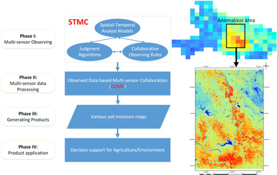
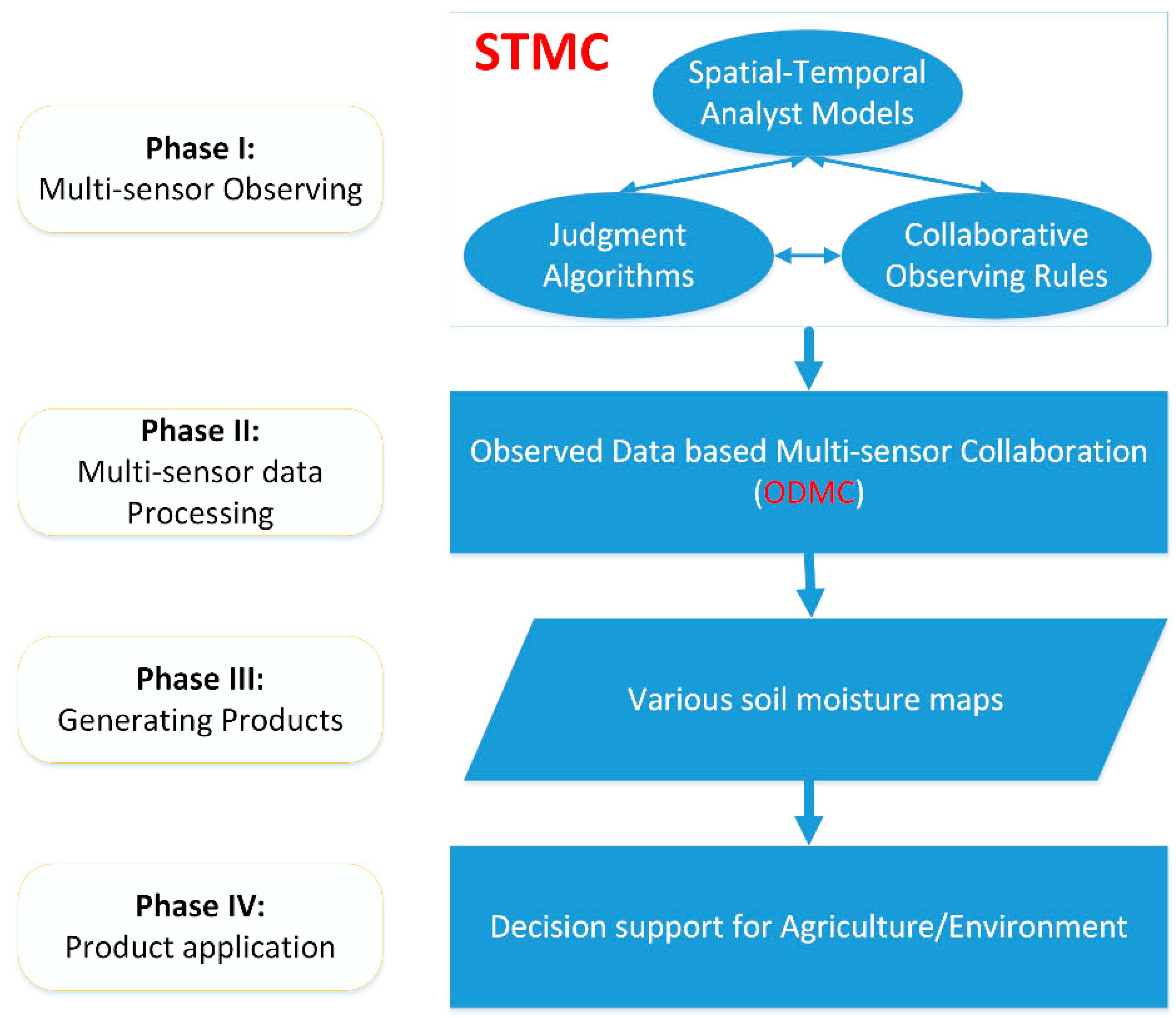
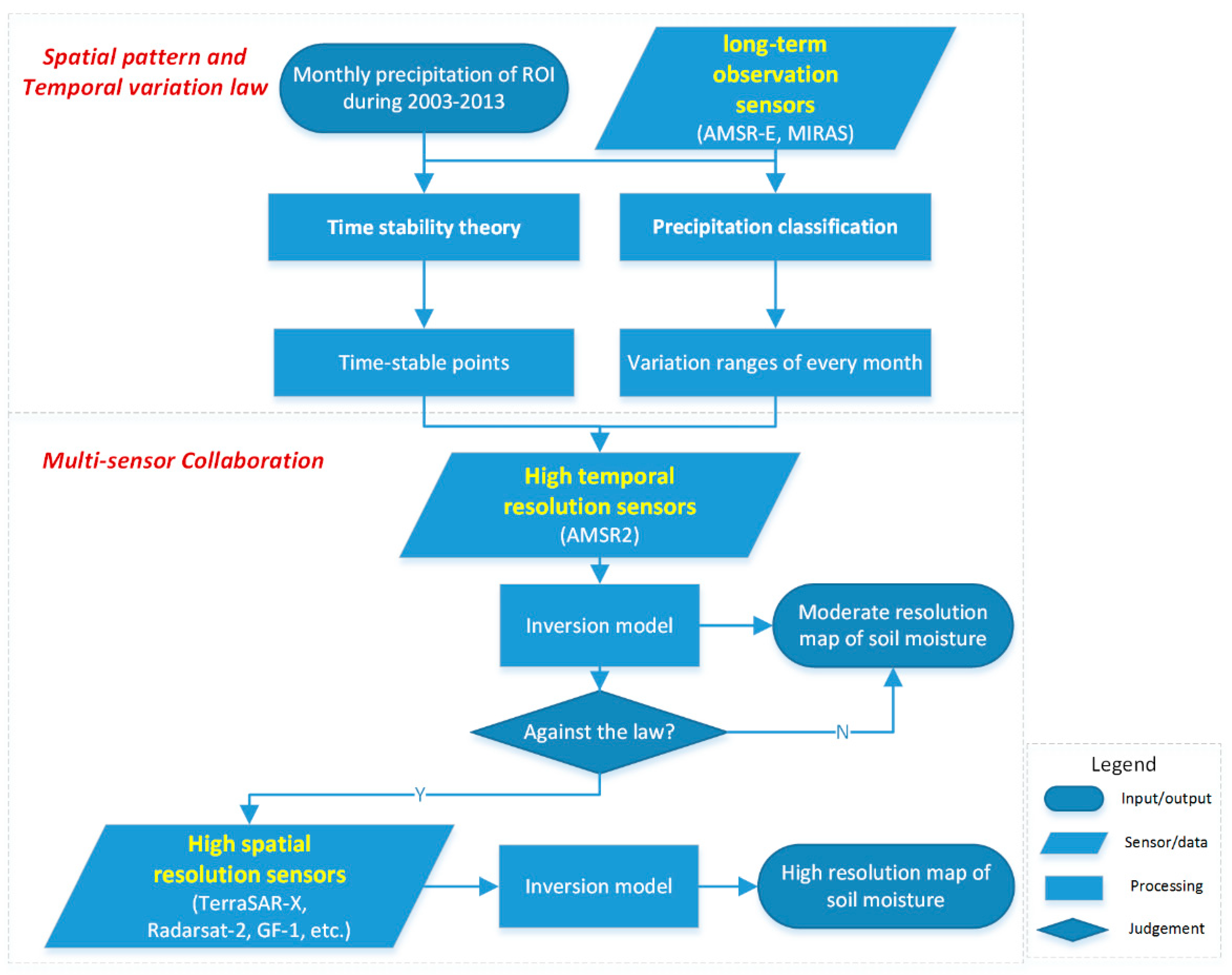
2.1. Overview of the STMC

According to the timeline shown in Figure 1, all of the soil moisture observations and applications can be divided into four phases, beginning with the observing phase and the ending with the application phase. The STMC method tries to improve the time efficiency in the observing phase to maximize the observation capabilities based on different sensors. After remote sensing data are collected via STMC, the ODMC method can help extract features and information in the data processing phase. Then, various soil moisture maps can be generated based on the user-defined or pre-defined requirements in the next phase. Subsequently, these products can be used in decision making for agriculture or environmental management.

Figure 1. The phases and concepts of the STMC method. The STMC method begins to achieve collaborative observations during the first phase. The spatial-temporal analyst models, judgment algorithms, and collaborative observing rules are important elements in the STMC method.

Figure 1. The phases and concepts of the STMC method. The STMC method begins to achieve collaborative observations during the first phase. The spatial-temporal analyst models, judgment algorithms, and collaborative observing rules are important elements in the STMC method.

These models, algorithms, and rules in the STMC method are shown in detail in Figure 2. The inputs required for the STMC method include the region of interest (ROI), the monthly precipitation from 2003 to 2013, and long-term observation data. The outputs of the STMC method include moderate- and high-resolution soil moisture maps. The entire STMC method was divided into two parts: (1) spatial-temporal patterns and temporal variation laws and (2) multi-sensor collaboration. The first part was used to construct a soil moisture distribution foundation for the judgment algorithms, and the second part was used to judge the anomalous soil moisture distribution and then organize the multi-sensor. Section 2.2 and Sections 2.3 described these two parts in detail. The only preconditions of the STMC method is that the vegetation type, terrain, soil composition, and cultivation method in study area must remain stable.

Figure 2. The flowchart of the proposed STMC method. The method is composed of two parts, the spatial pattern and temporal variation law extraction and the multi-sensor collaboration. Various remote sensors with different observation capabilities were orchestrated. These sensors included long-term observation sensors, high temporal resolution sensors, and high spatial resolution sensors.

Figure 2. The flowchart of the proposed STMC method. The method is composed of two parts, the spatial pattern and temporal variation law extraction and the multi-sensor collaboration. Various remote sensors with different observation capabilities were orchestrated. These sensors included long-term observation sensors, high temporal resolution sensors, and high spatial resolution sensors.

2.2. Spatial Pattern and Temporal Variation Law

After the ROI was defined, a long time series of remote sensing image data were collected for this region. The obtained images were derived from long-term observation sensors, including the Advanced Microwave Scanning Radiometer for EOS (AMSR-E) sensor onboard Aqua and the MIRAS sensor onboard Soil Moisture and Ocean Salinity. These long-term sensors have an advantage in data continuity and maturity. Thus, these sensors are quite suitable for extracting variation law over a long period. This is the first type of sensor that was used in collaboration within the STMC method.

Based on these long sequence data, the temporal stability/persistence method was utilized to obtain the spatial patterns of soil moisture distribution. Vachaud et al. [35] proposed the concept of time stability, which characterizes the time-invariant association between spatial location and the statistical parametric values of soil properties. In recent years, Jacobs et al. [36], Vivoni et al. [37], Zhao et al. [38], and Schneider et al. [39] indicated the importance of the time stability method for extracting soil moisture distribution trends. Therefore, data spanning a relatively long period, such as 120 images collected over the last 10 years, can be used to ensure that the relative accuracy of the soil moisture stability law can be deduced.

The time-stable point assessment uses θ_v,i, the volumetric soil moisture content (VSM) at location i for each sampling date [37], to calculate the regional mean as follows:

$$\overline{{\theta }_v^t}=\frac{1}{n_t}{\displaystyle \sum _{i=1}^{n_t}{\theta }_{v,i}}$$

(1)

where n_t is the number of points (the total pixels in each image) on a given date t = 1, 2, …, $N_t$ (the total number of sampling dates, such as 120), and θ_v,i is the soil moisture value of one pixel. The mean relative difference (MRD) (δ_i) for each sampling point [37] is calculated as follows:

$$\overline{{\delta }_i}=\frac{1}{N_t}{\displaystyle \sum _{t=1}^{N_t}\frac{{\theta }_{v,i}-\overline{{\theta }_v^t}}{\stackrel{-}{{\theta }_v^t}}}$$

(2)

The MRD of a pixel quantifies the pixel’s bias with time and identifies whether that location is wetter or drier than the regional average. Then, the variance of the relative difference (σ(δ_i)²) [37] is defined as follows:

$$\sigma {({\delta }_i)}^2=\frac{1}{N_t-1}{{\displaystyle \sum _{t=1}^{N_t}(\frac{{\theta }_{v,i}-\overline{{\theta }_v^t}}{\stackrel{-}{{\theta }_v^t}}-\overline{{\delta }_i})}}^2$$

(3)

Small values of σ(δ_i)² indicate time stable locations at which the relative wetness remains similar during the sampling period. Finally, the index of time stability (ITS_i) [38] is computed from the mean and variance as follows:

$${\text{ITS}}_{\text{i}}={({\overline{{\theta }_i}}^2+\sigma {({\delta }_i)}^2)}^{1/2}$$

(4)

The ITS provides a single metric for identifying the best locations that can capture the changes throughout the region. Using rank-ordered ITS_i, the point with the highest time-stability is identified as the one with the lowest ITS. An acceptable ITS threshold can be used to identify time-stable points (TSPs) within a region that consistently replicate the mean soil moisture within an allowable degree of error.

By using the time stability model, the calculation of soil moisture values on these selected TSPs is equivalent to the regional average soil moisture values. This time-stability based spatial pattern law is the foundation of soil moisture judgment algorithms in the next collaboration rules. Of course, there are many methods for judging variations in soil moisture. One simple solution is to compare the entire soil moisture image with the entire normal soil moisture image. However, this method is time-consuming, and the entire soil moisture image cannot be obtained if clouds present. The time stability method can be used to overcome this limitation by selecting limited TSPs to represent the spatial-temporal distribution of soil moisture over a long period. This method is important for obtaining a quick judgment of daily soil moisture variations. Thus, the STMC method combines time stability theory with long-term observation sensors.

Next, the STMC method calculates the temporal variation law of every TSP to obtain normal soil moisture ranges for every month. The soil moisture distribution is controlled by climate (precipitation and temperature), vegetation, terrain, soil composition, etc. Therefore, obtaining a normal soil moisture distribution level for one area at a specific time is a complicated process. However, in humid areas and for rain-fed arable lands, the soil moisture distribution is heavily influenced by precipitation. Thus, it is possible to derive soil moisture variation laws in these areas from mass historical precipitation data. First, we analyzed the monthly precipitation over the last ten years to obtain the mean monthly precipitation (p):

$$\overline{p}=\frac{{\displaystyle \sum _{i=1}^{N_t}{p}_i}}{N_t}$$

(5)

where N_t is the number of sampling months and p_i is the amount of precipitation in month i. Then, the anomaly precipitation for each month can be analyzed based on the precipitation anomaly percentage (PAP) as follows [40]:

$${\text{PAP}}_{\text{i}}=\frac{p_i-\overline{p}}{\overline{p}}*100\%$$

(6)

where PAP_i is the precipitation anomaly percentage of month i. Then, based on the PAP_i, the 120 months were classified into one of five classes, drought, weak drought, normal precipitation, light waterlogging, and waterlogging months [40]. The rules of classification are shown in Table 1.

Table 1. Rules for classifying different months with different soil moisture values.

Classification Factors	Classification Rules	Resulting in Soil Moisture
PAPi ≤ −20%	Drought month	Potential drought
−20% < PAPi ≤ −10%	Light drought month	Lower limit of normal soil moisture
−10% < PAPi < 10%	Normal precipitation month	Normal soil moisture month
10% ≤ PAPi < 20%	Light waterlogging month	Upper limit of normal soil moisture
PAPi ≥ 20%	Waterlogging month	Potential waterlogging

Table 1. Rules for classifying different months with different soil moisture values.

Classification Factors	Classification Rules	Resulting in Soil Moisture
PAPi ≤ −20%	Drought month	Potential drought
−20% < PAPi ≤ −10%	Light drought month	Lower limit of normal soil moisture
−10% < PAPi < 10%	Normal precipitation month	Normal soil moisture month
10% ≤ PAPi < 20%	Light waterlogging month	Upper limit of normal soil moisture
PAPi ≥ 20%	Waterlogging month	Potential waterlogging

Given that precipitation has the largest impact on soil moisture, normal precipitation months result in normal soil moisture levels. Weak drought months and weak flow months were chosen as the lower and upper normal limits of the normal soil moisture range. When these thresholds determined no weak drought months, the month with a PAP near −20% was chosen to calculate the lower limit. The same process was performed for the upper limit. These thresholds in the classification rules can be adjusted according to different study areas and requirements.

After analyzing the temporal variations of precipitation for every month during the last ten years, the historical soil moisture variations can be obtained. The use of passive microwave satellite sensors for estimating surface soil moisture values is a relatively mature and reliable technology. In addition, the soil moisture retrieval capabilities of the AMSR-E and MIRAS were widely discussed and validated [41,42,43]. Therefore, the soil moisture map or soil moisture values in every TSPs for all months can be easily obtained.

For every month, ten soil moisture images were obtained during ten years. These soil moisture images were classified into the five types listed above. When more than one weak drought images occurred within the month’s ten images, all weak drought months’ images were fused into one image to produce a synthetic lower limit of soil moisture for the TSPs. The same process was used for the images of all weak waterlogging months. To avoid the impacts of extreme values, we chose the median soil moisture value when fusing these images. Then, we applied this calculation from January to December. Finally, the range of soil moisture variations for every TSP for every month was derived as the following data range: [Lower limit, Upper limit]. The soil moisture was judged as normal if its value was in this range. Therefore, we obtained 12 variation ranges for every TSP. These ranges can be valuable for judging potential drought or waterlogging crises.

To illustrate the above spatial pattern and temporal variation laws extraction more clearly, Figure 3 shows method details. In the next portion of the STMC method, the daily changes in soil moisture of a single region are detected and evaluated based on this law.

Figure 3. The flowchart showing how the STMC method extracts the spatial pattern and temporal variation laws based on long sequence remote sensing images and historical precipitation data. One parameter of 200 x, 200 y, 200 m, 200 n, 200 a, 200 b, 200 c, 200 d, 200 e, 200 f, 200 g, and 200 h represents one year between 2003 and 2013.

Figure 3. The flowchart showing how the STMC method extracts the spatial pattern and temporal variation laws based on long sequence remote sensing images and historical precipitation data. One parameter of 200 x, 200 y, 200 m, 200 n, 200 a, 200 b, 200 c, 200 d, 200 e, 200 f, 200 g, and 200 h represents one year between 2003 and 2013.

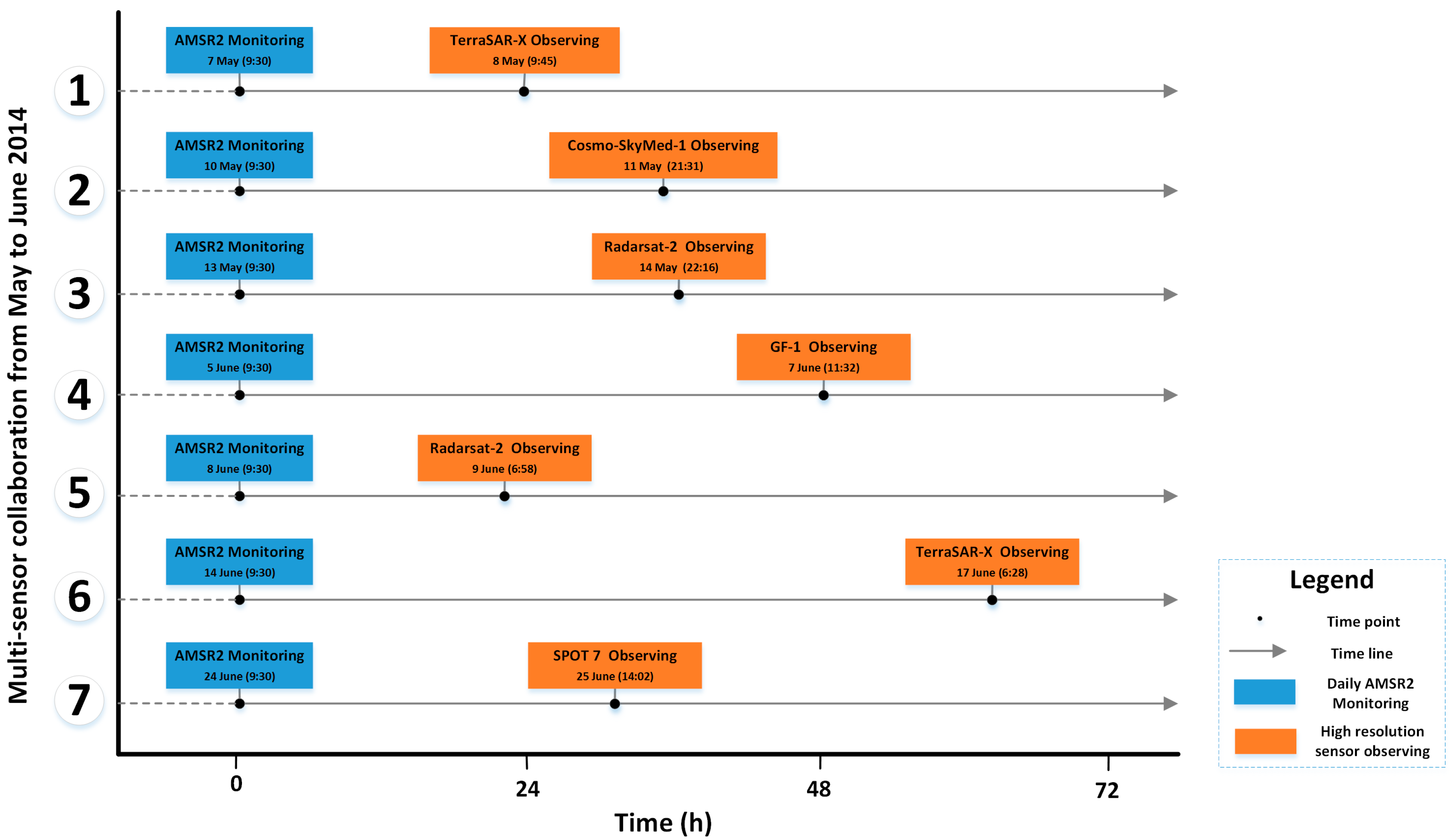
2.3. Multi-Sensor Collaboration

After the spatial pattern and temporal variation law of soil moisture was established for the ROI, other sensors with different observation capabilities were then orchestrated to monitor the regional soil moisture contents.

First, the STMC method takes advantages of high temporal resolution sensors to achieve near real-time monitoring. The Advanced Microwave Scanning Radiometer 2 (AMSR2) onboard the GCOM-W satellite can measure microwave emission from the surface. The antenna of AMSR2 rotates once per 1.5 s and obtains data over a 1450 km swath. This conical scan mechanism allows AMSR2 to acquire a set of daytime and nighttime data with more than 99% coverage of the Earth every 2 days. In addition, the AMSR2 instrument is a dual polarized total power microwave radiometer system with six frequency bands ranging from 7 GHz to 89 GHz [44]. Therefore, the AMSR2 contributes to daily soil moisture monitoring, regardless of cloud cover during the day and night. Thus it provides a more powerful near real time monitoring tool compared with other optical sensor (i.e., MODIS) in areas with heavy rainfall. This is the second type of sensor that we collaborate in the STMC method.

After obtaining a moderate-resolution map of soil moisture for one day, a judgment algorithm is triggered to determine whether the determined soil moisture distribution corresponds with the soil moisture distribution law. Because of the TSPs and variation ranges derived in the first part, the judgment algorithm only requires checking the soil moisture values of these TSPs. In the STMC method, the anomalous soil moisture judgment algorithm (ASMJ algorithm) determines and locates the areas with anomalous soil moisture. The ASMJ algorithm is illustrated in Figure 4.

Figure 4. Details regarding the ASMJ algorithm. The TSPs and variation ranges are used to judge the normal or anomalous soil moisture distributions in the region. The change detection is used to target the anomalous areas. The role of the ASMJ algorithm in the STMC method is illustrated in the lower left. The parameter m is the number of TSPs whose values are against normal soil moisture value ranges. And the parameter n is the total number of TSPs.

Figure 4. Details regarding the ASMJ algorithm. The TSPs and variation ranges are used to judge the normal or anomalous soil moisture distributions in the region. The change detection is used to target the anomalous areas. The role of the ASMJ algorithm in the STMC method is illustrated in the lower left. The parameter m is the number of TSPs whose values are against normal soil moisture value ranges. And the parameter n is the total number of TSPs.

First, the ASMJ algorithm obtains the soil moisture values of n TSPs. Next, it compared these values with the normal variation ranges ([Lower limit, Upper limit]) of the given month for every TSP. By examining these ranges and values, the number of points with values outside of the expected soil moisture ranges was m.

Then, a threshold (n/3) was used to judge how many anomalous soil moisture values existed in the region. Of course, this threshold could be adjusted according to different monitoring requirements. For example, if the region has a high priority and the region’s dynamic soil moisture changes must be monitored more carefully, then the threshold can be set to n/5. Here, n/3 was chosen to balance efficiency and cost.

When m ≤ n/3, no anomalous soil moisture areas are found in the region. Therefore, the former moderate-resolution soil moisture map is adequate for regular monitoring. However, when m>n/3, an anomalous soil moisture distribution occurs in the region.

To avoid short-duration anomalous soil moisture events, a threshold (p) was added to account for the time duration of anomalous soil moisture events. When p < 3, the event only features temporary anomalous changes over a short period. However, when p ≥ 3, the soil moisture levels have exceeded the normal ranges for more than three days.

Once the soil moisture levels have exceeded the normal ranges for more than three days, a change detection method is used to compare the daily soil moisture map with the lower-limit fused map and the upper-limit fused map. Following this change detection process, the anomalous areas, including drought and waterlogged areas, are located. Therefore, the ASMJ algorithm judges and targets the locations of anomalous soil moisture areas.

If the ASMJ algorithm detects anomalous areas successfully, high-resolution/capability sensors are immediately triggered to obtain detailed soil moisture data for the targeted areas. High spatial resolution optical sensors and SAR sensors can provide more detailed and accurate soil moisture monitoring capabilities. However, their swaths are relatively narrow and their return cycles are relatively long. Therefore, scheduling a high-resolution satellite sensor to monitor regional soil moisture is expensive in terms of observation opportunities and cost. Thus, with the help of moderate AMSR2 sensor, high-resolution sensors can be utilized efficiently. Hence, these high-resolution sensors are the third type of sensor we collaborate in STMC method.

Based on the ASMJ algorithm, the STMC method selects and sends an observation request to high-resolution sensors (such as the sensors onboard TerraSAR-X, Radardsat-2, and GF-1) for the right time and place. This selection criterion is flexible. For example, the STMC method can choose the nearest satellite sensor that can pass the target area within the shortest time. Therefore, a high-resolution soil moisture map can be obtained quickly. Under other conditions, the STMC method can also choose the low cost high-resolution sensor. Anyhow, this timely high-resolution map can provide detailed information for decision makers to analyze and handle anomalous changes of regional soil moisture.

Therefore, the ASMJ algorithm in the STMC method solves three monitoring questions: (1) how to determine anomalous soil moisture changes (TSPs and m), (2) how to identify a severe soil moisture event (p), and (3) and how to extract anomalous soil moisture areas (change detection). These collaborative sensing rules balance the multi-sensor observation order and selection in terms of moderate spatial resolution sensors with a high return frequency and high spatial resolution sensors with a low return frequency.

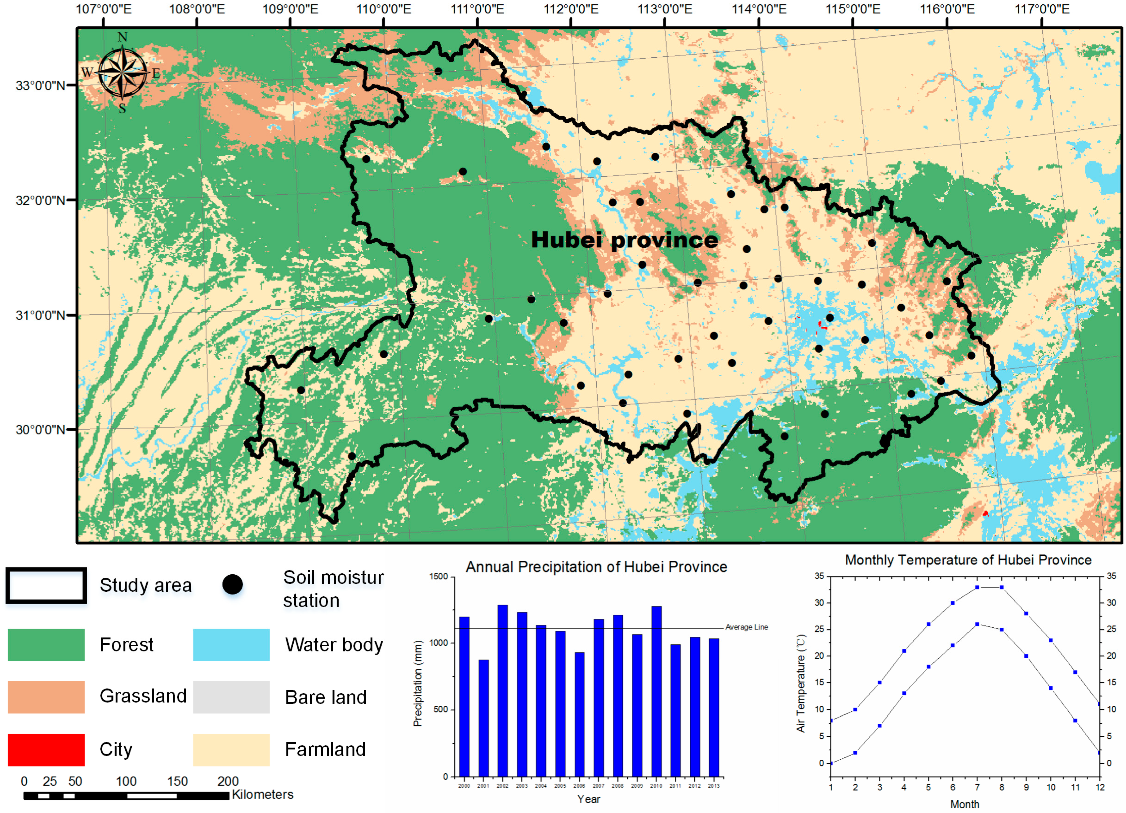
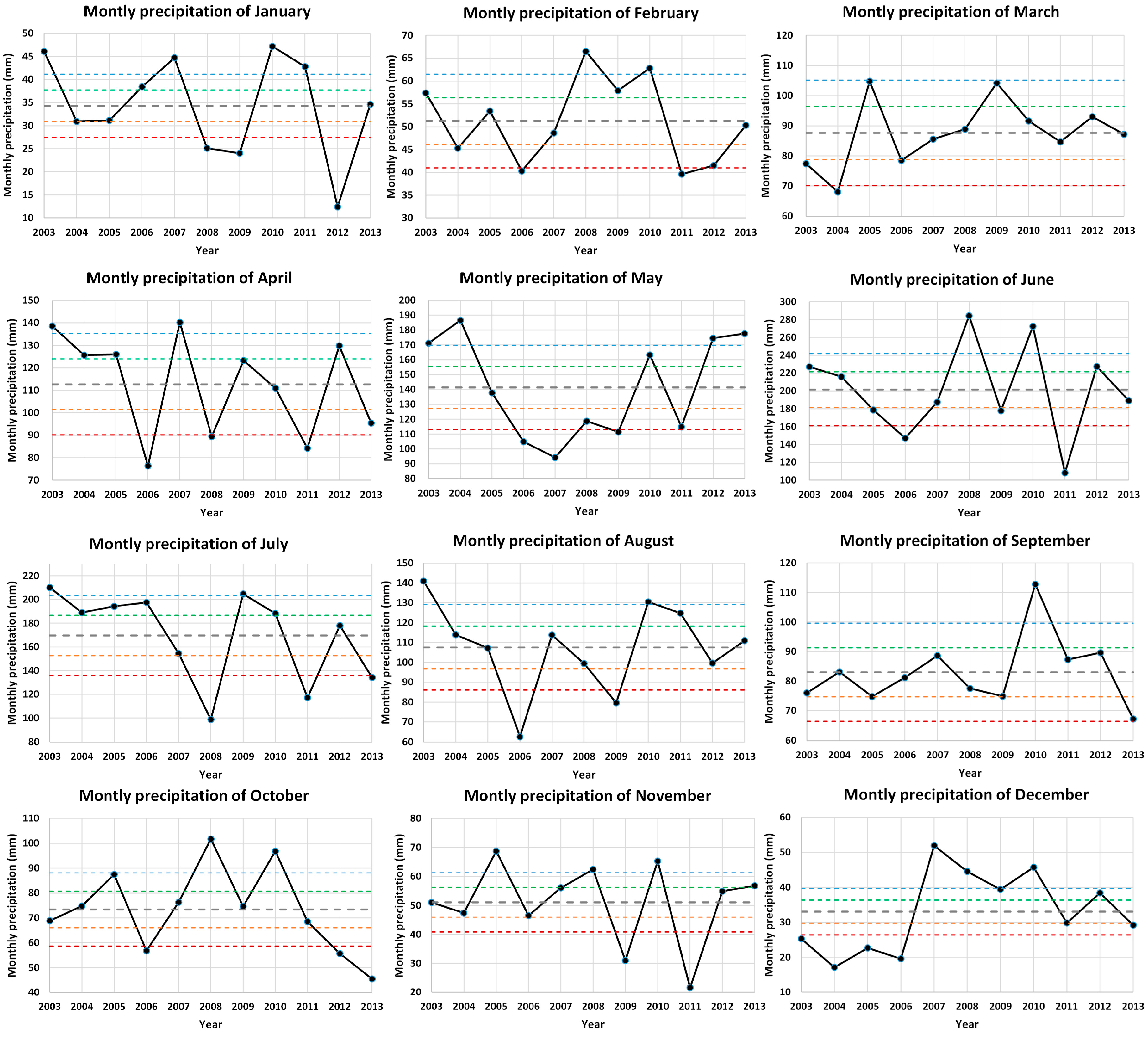
3. Study Area and Dataset

As shown in Figure 5, the study area (Hubei province) is located in the easternmost region of Central China (108°21′E–116°07′E longitude and 29°05′N–33°20′N latitude). The Jianghan Plain takes up most of central and southern Hubei (20%), and hills (24%) and mountains (56%) are present in the west and in the peripheral areas. Hubei province is approximately 185,900 km² and contains 57.79 million people. This area has a subtropical humid monsoon climate with obvious continental climate features, and 1110–2150 sunshine hours. The annual average precipitation varies from 814.5 mm to 1627.0 mm, and its annual average temperature varies between 15 °C and 17 °C. In 2013, the GDP of Hubei province was 2466.849 billion, with 309.816 billion added by the first industries, such as farming, forestry, animal husbandry and aquaculture. Therefore, Hubei province is often called the “Land of Fish and Rice”.

Figure 5. The experimental region (Hubei province) and land use. The western portion of Hubei province is covered by mountains and hills, and the eastern portion is covered by farmland. In addition, two rivers (Yangtze River and Hanjiang River) flow through this region. The black points indicate in situ meteorological stations for measuring soil moisture at the surface.

Figure 5. The experimental region (Hubei province) and land use. The western portion of Hubei province is covered by mountains and hills, and the eastern portion is covered by farmland. In addition, two rivers (Yangtze River and Hanjiang River) flow through this region. The black points indicate in situ meteorological stations for measuring soil moisture at the surface.

However, Hubei province is seriously affected by soil moisture related disasters, such as droughts and floods. In 2011, the great drought resulted in up to 7.47 billion in economic losses in Hubei province, with affected an area of more than 667, 000 hm². Therefore, the distribution and variation of soil moisture in Hubei province is important for supporting agricultural and for environmental decision-making. The STMC method was tested in this region to improve soil moisture monitoring based on multiple sensors from May to June 2014.

Overall, 120 images of Hubei province (the ROI) were collected from 2003 to 2013. These data were made up of AMSR-E and MIRAS images. The AMSR-E antenna stopped spinning on 4 October 2011. Thus, MIRAS was used to ensure that the ten-year soil moisture images were complete. To avoid multi-scale problems in daily soil moisture judgment with AMSR2, these data resampled to 30 km. To avoid the influences of soil moisture changes between day and night, all of the data were obtained from the morning pass (approximately 9:30). Based on these long-time series of microwave data, the spatial pattern and temporal variation laws of the soil moisture in the study region were obtained.

In Table 2, the monthly precipitation data in Hubei province were obtained for 2003 to 2013. These precipitation data were provided by the meteorological bureau of Hubei province. The temporal variation law of soil moisture in the study region was deduced from the monthly precipitation data.

Table 2. Monthly precipitation in Hubei province from 2003 to 2013.

Year	Monthly Precipitation in Hubei Province (mm)
	Jan.	Feb.	Mar.	Apr.	May	Jun.	Jul.	Aug.	Sep.	Oct.	Nov.	Dec.
2003	46.1	57.4	77.4	138.5	171.2	227.2	210.1	141.0	76.0	68.9	51	25.3
2004	30.9	45.3	68.1	125.6	186.6	215.9	189.0	113.9	83.1	74.8	47.4	17.1
2005	31.1	53.4	104.8	125.9	137.8	178.8	194.3	107.2	74.8	87.5	68.7	22.7
2006	38.4	40.3	78.5	76.3	104.9	147.2	197.5	62.6	81.2	56.8	46.5	19.6
2007	44.7	48.6	85.6	140.2	94.2	187.5	154.4	113.8	88.6	76.3	56.1	51.9
2008	25.1	66.5	88.9	89.4	118.7	284.4	98.8	99.4	77.5	101.7	62.4	44.5
2009	24.0	57.9	104.2	123.2	111.5	177.9	204.7	79.6	74.9	74.6	31.0	39.4
2010	47.2	62.8	91.6	110.9	163.3	272.6	188.2	130.5	112.8	96.8	65.3	45.7
2011	42.8	39.6	84.7	84.2	114.9	108.3	117.3	124.8	87.3	68.5	21.6	29.8
2012	12.4	41.5	93.0	129.8	174.6	227.5	178.1	99.6	89.6	55.7	54.9	38.4
2013	34.6	50.3	87.2	95.4	177.7	189.3	134.2	110.9	67.2	45.5	56.8	29.2

Table 2. Monthly precipitation in Hubei province from 2003 to 2013.

Year	Monthly Precipitation in Hubei Province (mm)
	Jan.	Feb.	Mar.	Apr.	May	Jun.	Jul.	Aug.	Sep.	Oct.	Nov.	Dec.
2003	46.1	57.4	77.4	138.5	171.2	227.2	210.1	141.0	76.0	68.9	51	25.3
2004	30.9	45.3	68.1	125.6	186.6	215.9	189.0	113.9	83.1	74.8	47.4	17.1
2005	31.1	53.4	104.8	125.9	137.8	178.8	194.3	107.2	74.8	87.5	68.7	22.7
2006	38.4	40.3	78.5	76.3	104.9	147.2	197.5	62.6	81.2	56.8	46.5	19.6
2007	44.7	48.6	85.6	140.2	94.2	187.5	154.4	113.8	88.6	76.3	56.1	51.9
2008	25.1	66.5	88.9	89.4	118.7	284.4	98.8	99.4	77.5	101.7	62.4	44.5
2009	24.0	57.9	104.2	123.2	111.5	177.9	204.7	79.6	74.9	74.6	31.0	39.4
2010	47.2	62.8	91.6	110.9	163.3	272.6	188.2	130.5	112.8	96.8	65.3	45.7
2011	42.8	39.6	84.7	84.2	114.9	108.3	117.3	124.8	87.3	68.5	21.6	29.8
2012	12.4	41.5	93.0	129.8	174.6	227.5	178.1	99.6	89.6	55.7	54.9	38.4
2013	34.6	50.3	87.2	95.4	177.7	189.3	134.2	110.9	67.2	45.5	56.8	29.2

4. Experiment Results

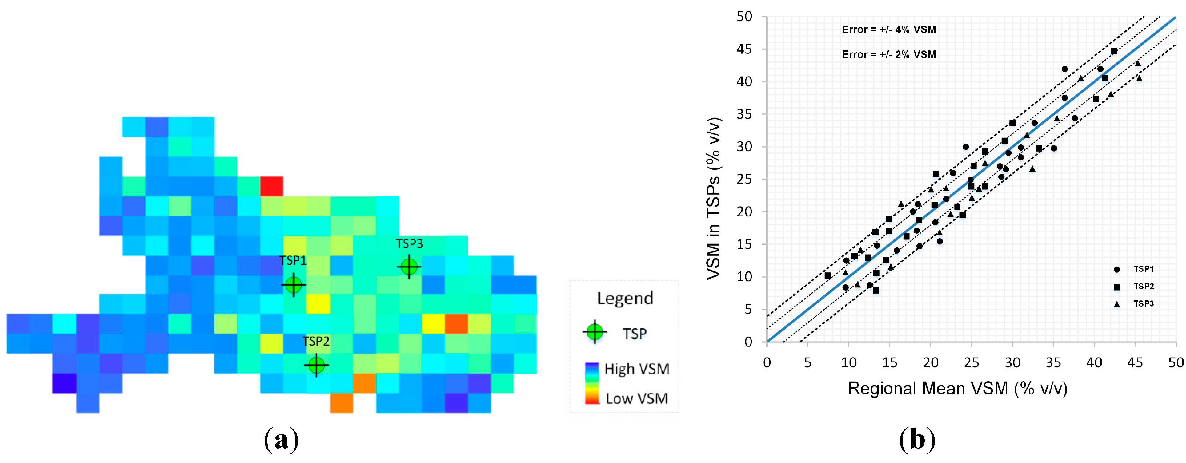
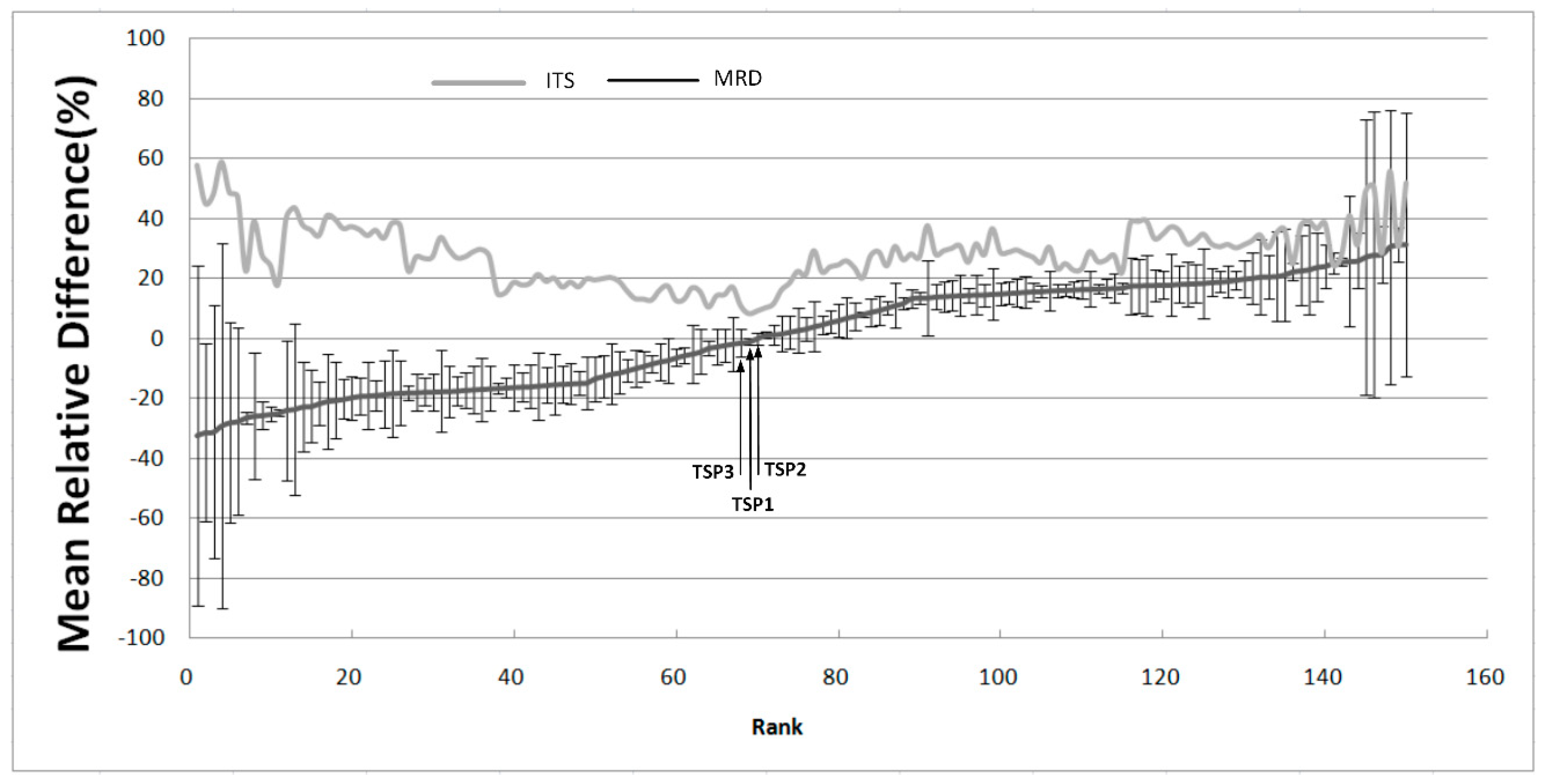
4.1. Spatial Pattern Law of Soil Moisture

If a region exhibits time-stable characteristics, these TSPs can offer an efficient way to represent the spatial distribution of soil moisture in this region. Based on the analyses of 120 soil moisture images between 2003 and 2013, Figure 6 shows time-stability characteristics (MRD) (ranked from the smallest to the largest) and the ITS values for pixels in the region.

The pixels/points with negative MRD values consistently underestimate the region average. While the points with positive values consistently overestimate the regional average. These results indicate that a number of satisfactory TSPs are available for this study region. Three points with ITS values near zero were chosen to represent the regional average soil moisture contents in the study region. Figure 7a shows the locations of the selected three TSPs in the region. It was found that these three TSPs, named TSP1, TSP2, and TSP3 were located in the middle area between the hills and lakes. According to Jacobs et al. [36] the time stability of points with mild slopes and moderate to moderately high clay contents consistently exhibited stable features. In the study area, the yellow brown soil is widely distributed across the farmland. Therefore, our findings are consistent with the former research.

Figure 7b shows that the agreement of volumetric soil moisture (VSM) in TSPs with regional mean VSM. It was found that, the majority (86.1%) of the 72 checkpoints lay between the −4% error line and the +4% error line. Therefore, these TSPs provide an accurate estimation of the mean field value with low variability and a small bias.

Figure 6. Rank-ordered MRD of the volumetric soil moisture and ITS for 150 points in the study area from 2003 to 2013. The vertical bars correspond to the associated MRD standard deviations. The light grey curve indicates the ITS, and the labeled points have the minimum ITSs.

Figure 6. Rank-ordered MRD of the volumetric soil moisture and ITS for 150 points in the study area from 2003 to 2013. The vertical bars correspond to the associated MRD standard deviations. The light grey curve indicates the ITS, and the labeled points have the minimum ITSs.

Figure 7. (a) The locations of the selected three TSPs in the region. (b) Comparison of the regional mean soil moisture versus the soil moisture values of the three TSPs.

Figure 7. (a) The locations of the selected three TSPs in the region. (b) Comparison of the regional mean soil moisture versus the soil moisture values of the three TSPs.

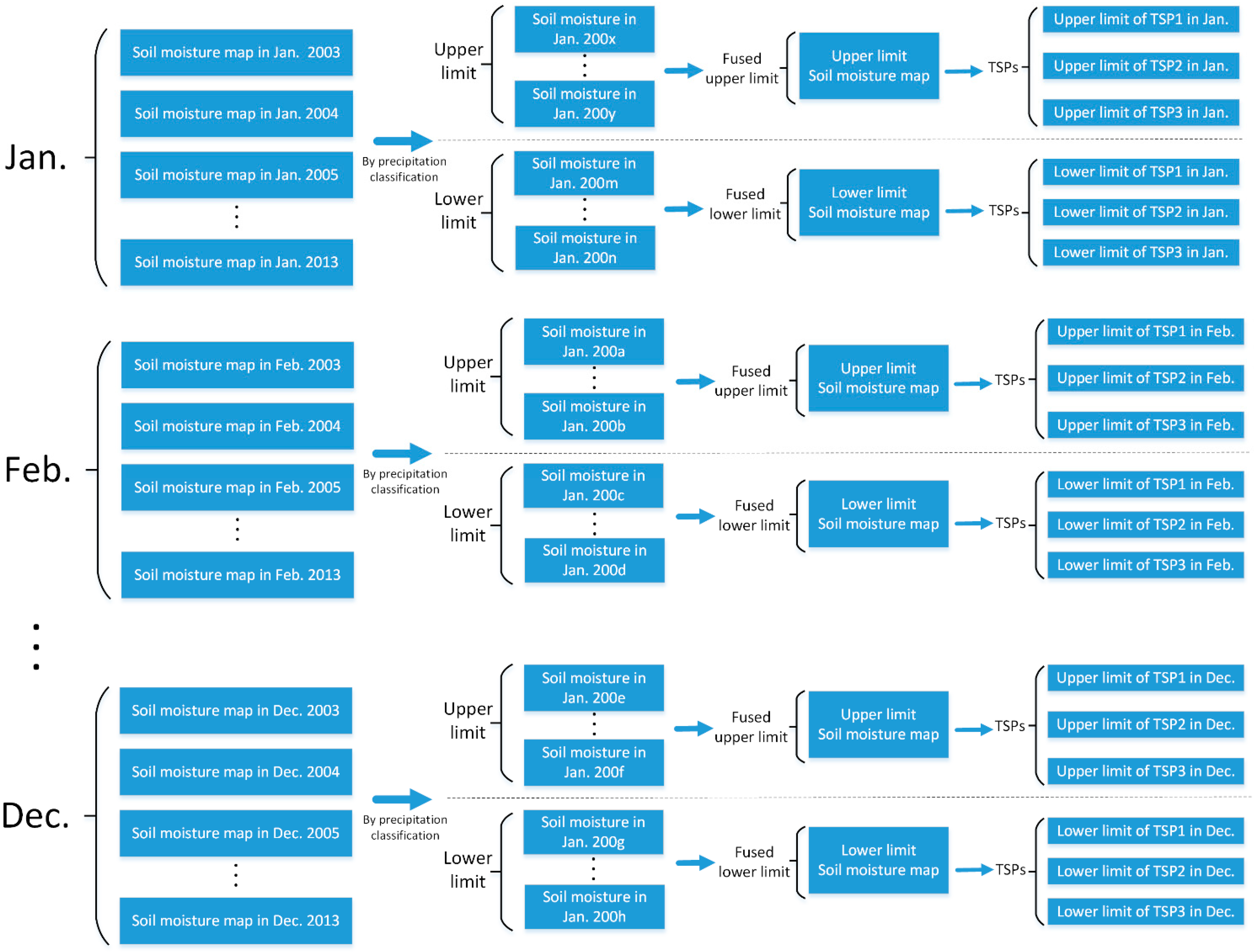
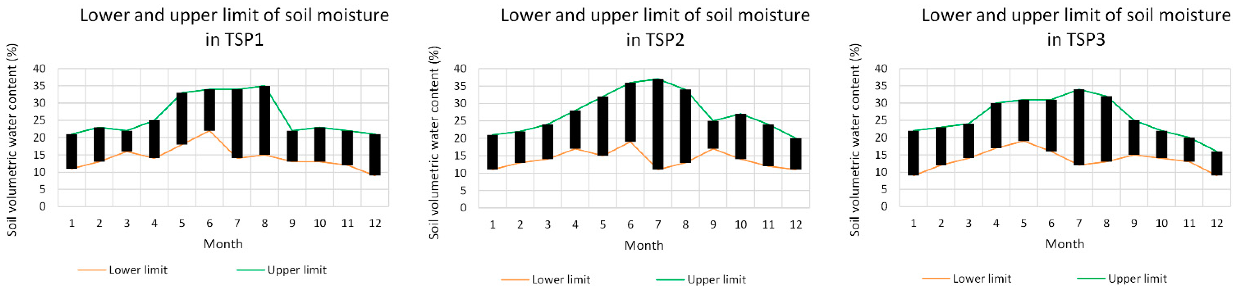
4.2. Temporal Variation Law of Soil Moisture

The p and PAP values of every month between 2003 and 2013 were analyzed and were shown in Figure 8. It was found that the precipitation variations of every month were different, but the PAP was used to help classify these months into different types. According to the classification rules shown in Table 1, the normal variations ([Lower limit, Upper limit]) of every TSP were derived from the soil moisture values during the weak drought months and weak waterlogging months. For example, the lower limit of the variation range in January was calculated from the soil moisture in January 2004, whereas the upper limit occurred in 2006. The lower limit of the variation range in February resulted from the fusion of the soil moisture data from 2004 and 2012, whereas the upper limit resulted from the fusion of the soil moisture data from 2003 and 2009.

Figure 8. Monthly precipitation, the monthly mean precipitation (MMP) line, the 20% PAP line, the 10% PAP line, the −10% PAP line, and the −20% PAP line from 2003 to 2013.

Figure 8. Monthly precipitation, the monthly mean precipitation (MMP) line, the 20% PAP line, the 10% PAP line, the −10% PAP line, and the −20% PAP line from 2003 to 2013.

Therefore, the variation range of every TSP in every month was calculated. Figure 9 shows the soil moisture ranges for TSP1, TSP2, and TSP3. For example, if soil moisture value of TSP1 is between 11% and 21% in January, it is judged to be normal soil moisture in this TSP. Similarly, if soil moisture value of TSP1 is not within 14% to 34% in July, the soil moisture distribution in this study region may be anomalous. In addition, the variation scales were different in different months. For example, the variations ranges in December, January, February, and March were smaller than in July and August. This result is related to the more static meteorology conditions in the spring and winter and to larger precipitation variations and higher evaporation in the summer. Overall, the variation ranges in these three TSPs were very similar.

Figure 9. Variation range of every TSP for every month.

Figure 9. Variation range of every TSP for every month.

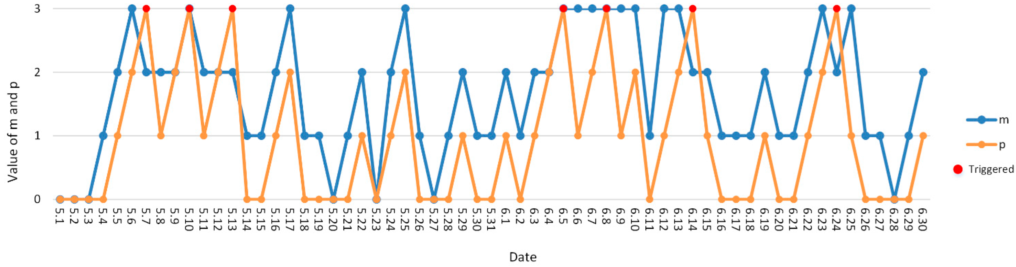
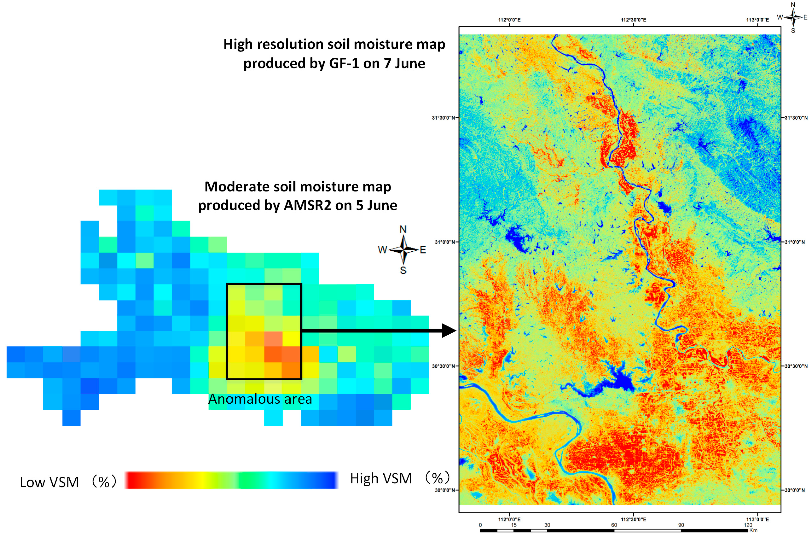
4.3. Multi-Sensor Collaboration for Hubei Province Soil Moisture Monitoring

From May to June in 2014, the STMC method was used in the study area. The daily AMSR2 image was used to extract the soil moisture values of the three TSPs. Then, the ASMJ algorithm was utilized to judge the anomalous soil moisture events. The details of the ASMJ algorithm result are illustrated below in Figure 10. The m and p parameter values varied during the study period. According to the judgment rules defined in the ASMJ algorithm, when p ≥ 3, the soil moisture distribution has remained anomalous for a relatively long time. In Figure 10, anomalous distributions were detected seven times (red dots): 7 May, 10 May, 13 May, and 5 June, 8 June, 14 June, and 24 June.

Figure 10. The m and p values of the ASMJ algorithm between May 2014 and June 2014. Long durations of anomalous values of m resulted in the value of p that were greater than or equal to 3. Then, an anomalous soil moisture event was detected and high-resolution satellite sensors were triggered. Overall, seven times (red dots) were judged to be anomalous soil moisture events.

Figure 10. The m and p values of the ASMJ algorithm between May 2014 and June 2014. Long durations of anomalous values of m resulted in the value of p that were greater than or equal to 3. Then, an anomalous soil moisture event was detected and high-resolution satellite sensors were triggered. Overall, seven times (red dots) were judged to be anomalous soil moisture events.

In Figure 10, from 1 May and 7 May it was observed that the value of m increased from 0 to 3. This increment resulted in a value growth of p. When p reached 3 on 7 May, the STMC method indicated that an anomalous soil moisture distribution event occurred. Under this condition, a high-resolution observation request was triggered. After 7 May, the value of m varied between 2 and 3, which indicated that the anomalous soil moisture distribution still existed in Hubei province. Therefore, two high-resolution observation requests were triggered on 10 May and 13 May. According to the historical weather data, a heavy rain event occurred between 9 May and 11 May in south and east of Hubei province (Xianning City, Huangshi City, Ezhou City, etc.). The daily precipitation was between approximately 100 and 150 mm. This event caused the waterlogging in this region. After the rainfall decreased, the soil moisture returned to normal. These results showed that the ASMJ algorithm was of value to capture the soil moisture variations in the region.

Between 14 May and 4 June, it was found that the value of m fluctuated. For example, the value of m was 2 on 16 May and 3 on 17 May. This change indicated that the soil moisture content was temporally anomalous. However, the duration of this anomaly was short, and m decreased back to 1 on 18 May. According to historical weather data in Hubei province, a moderate rain event occurred on 16 May and 17 May that stopped on the 18 May. In addition, on 25 May, heavy rain occurred west and north of Hubei province (Yichang City, Xiangyang City, and Xiaogan City). Therefore, the dynamic soil moisture level can be efficiently detected by using parameter m, and the p parameter is valuable for determining relatively long-duration changes. This character is useful for filtering temporally short soil moisture fluctuations and for reporting more critical anomalous soil moisture distribution alerts. Of course, the threshold of p can be adjusted according to different user requirements.

From 2 June to 15 June, it was found that the value of m increased from 1 to 3, and the value of p increased to 3 on three different occasions. This pattern indicated that the situation of anomalous soil moisture existed for a long time. Therefore, three high-resolution sensor-planning requests were triggered to obtain detailed observations for this region. After 15 June, the value of m decreased, and the soil moisture returned to its normal levels or temporal anomalous. In addition, on 24 June, the soil moisture distribution was judged as anomalous again. Based on historical weather data in Hubei province, no rain occurred in this region from 2 June, and the average temperature reached up to 30.5 °C, especially in central area. Consequently, a small drought occurred and was successfully captured by the ASMJ algorithm. From 16 June to 21 June, the majority of Hubei province was covered by clouds and experienced light rainfall. These weather changes reduced the impact of the drought.

To illustrate which sensors were used in this multi-sensor collaboration experiment, a visualization of the seven timelines for the seven collaboration scenarios was shown in Figure 11 (from top to bottom). Each scenario’s timeline features daily AMSR2 acquisition time points and the observation time points obtained by high-resolution sensors with the soonest pass-over time.

It was found that the daily AMSR2 sensor cooperated well with the high resolution sensors to obtain a quick and fine look on the targeted area. For example, in scenario 1, the soil moisture in the study region was judged to be anomalous after analyzing the daily AMSR2 data with ASMJ algorithm on 7 May. Then, the STMC method selected and requested high-resolution sensors to monitor the targeted area. TerraSAR-X was chosen to perform rapid data acquisition immediately. Therefore, high-resolution soil moisture maps were obtained by using the TerraSAR-X SAR sensor on the following day. One benefit of this collaborative monitoring rule is that, the high-resolution TerraSAR-X data values are increased due to the urgent demand for detailed regional monitoring data. Besides that, the time delay by obtaining these multi-scale remote sensing data is shortened by this automatic driven mechanism. The STMC method only required about 24 h to 72 h from the detection of anomalous soil moisture conditions to high-resolution soil maps in this experiment.

Figure 11. An overview of the local time points of the daily AMSR2 acquisitions and high-resolution data acquisitions in the study area.

Figure 11. An overview of the local time points of the daily AMSR2 acquisitions and high-resolution data acquisitions in the study area.

Figure 12. The moderate- and high-resolution soil maps were obtained by using the STMC method on 5 June and 7 June.

Figure 12. The moderate- and high-resolution soil maps were obtained by using the STMC method on 5 June and 7 June.

For these seven scenarios, high-resolution remote sensing data could not be acquired effectively without identifying the anomalous soil moisture areas using the ASMJ algorithm. Of course, although SMTC method chosen the high-resolution sensors with the soonest pass-over time, some scenarios with time intervals of approximately 48 h were observed. As soil moisture-related disasters, such as waterlogging or drought have slow onsets. Therefore, this time lag is acceptable for monitoring soil moisture.

Finally, high-resolution soil moisture maps were obtained to support agricultural and environmental decision-making. Figure 12 shows the moderate-resolution soil moisture map of the study area that was mapped on 5 June, and shows one anomalous area that was detected by the ASMJ algorithm. Then, the high-resolution soil map was produced by the wide field camera aboard the GF-1 satellite on 7 June, which had a spatial resolution of 16 m.

5. Discussion

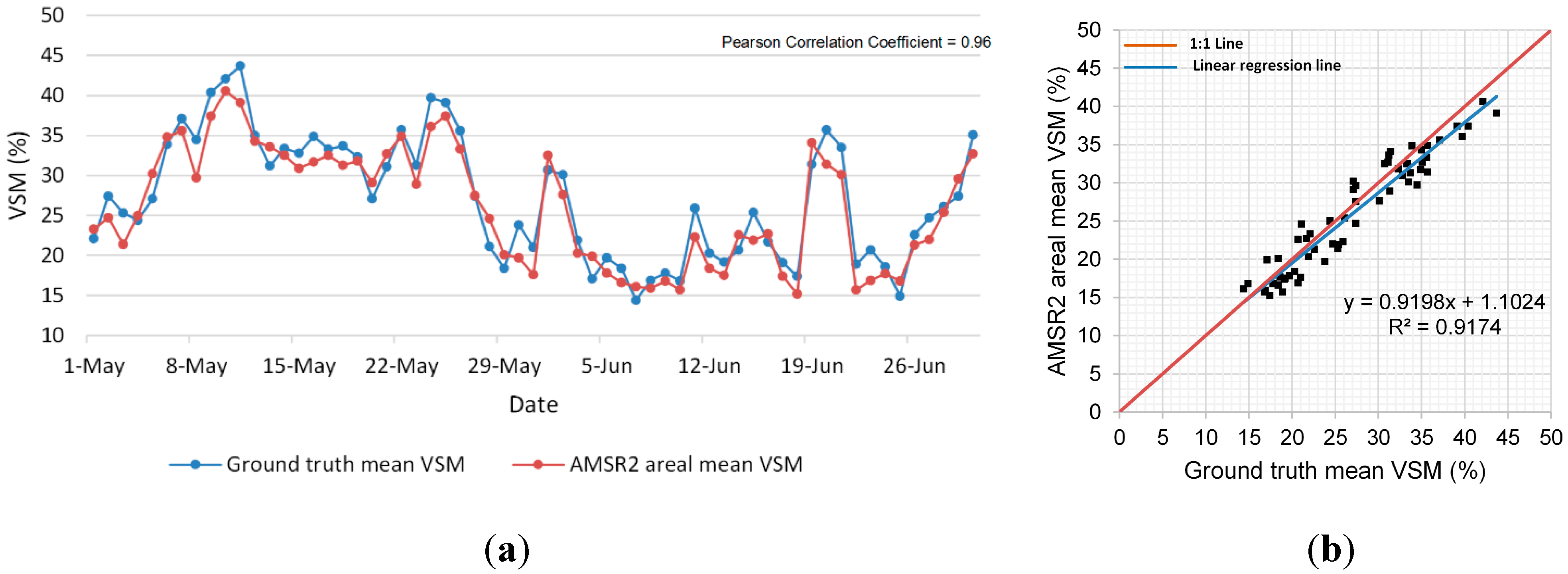
5.1. Accuracy Test of Daily AMSR2 Monitoring

The accuracy of daily AMSR2 L3 soil moisture products is important for judging the anomalous soil moisture distribution in the ASMJ algorithm. Therefore, we tried to evaluate the accuracy using in situ observation data. As shown in Figure 5, 45 in situ meteorological stations were distributed over the study area and were used to measure soil moisture at a depth of 5 cm. We collected these in situ data at 10 a.m. every day from 1 May to 31 June. Then, the Pearson’s correlation analysis was conducted between the ground truth mean VSM and AMSR2 VSM. In Figure 13a, the analysis showed that the Pearson’s correlation coefficient was approximately 0.96. These results suggested that the quality of the AMSR2 L3 soil moisture products was good, which was a solid foundation for the STMC method. From Figure 13b, it was found that though high correlation (R² = 0.9174) was between these two data, the AMSR2 slightly underestimated soil moisture.

Figure 13. (a) The correlation analysis of mean VSM of ground truth and AMSR2. (b) The regression line and 1:1 line based on mean VSM of ground truth and AMSR2.

Figure 13. (a) The correlation analysis of mean VSM of ground truth and AMSR2. (b) The regression line and 1:1 line based on mean VSM of ground truth and AMSR2.

5.2. Comparison with the ODMC Method

After successfully obtaining data from multi-sensor in the above experiment, the traditional ODMC method can continue to utilize these multisource images. It is important to compare these two methods from several factors. The targeted phase, method input, focus object, method output, and the headroom of ODMC and STMC methods are summarized in Table 3.

Table 3. Approaches comparison between the traditional ODMC method and the proposed STMC method from five aspects: phase, input, focus, output, and headroom.

Aspects	ODMC Method	STMC Method
Phase	Data application	Data acquiring
Input	Multi-sensor’s data	Multi-sensor’s Observation capabilities
Focus	Assimilation model, fusion algorithms	Observation strategy
Output	More valuable processed data or information	More efficient and timely multi-sensor’s raw data or information
Headroom	Middle	High

Table 3. Approaches comparison between the traditional ODMC method and the proposed STMC method from five aspects: phase, input, focus, output, and headroom.

Aspects	ODMC Method	STMC Method
Phase	Data application	Data acquiring
Input	Multi-sensor’s data	Multi-sensor’s Observation capabilities
Focus	Assimilation model, fusion algorithms	Observation strategy
Output	More valuable processed data or information	More efficient and timely multi-sensor’s raw data or information
Headroom	Middle	High

It was shown that the ODMC method took advantages of various data and provided more valuable data for applications than a single data resource. In the above experiment, the ODMC can fuse these multi-scale images or assimilate these soil moisture values into models. However, the proposed STMC method focuses on the sensor observation stage to achieve collaborative observations. Therefore, the aim of the STMC method is to enhance the utilization efficiency of various sensors with different observation capabilities. In the above experiment, the STMC method was demonstrated as a new collaborative soil moisture-monitoring scheme with diverse observation capabilities.

Therefore, the “collaboration” in the STMC method represents a new observation strategy contributed by multiple sensors to determine the regional soil moisture. The values of multiple sensors are limited if we think of them as individual sensors. Therefore, the STMC method attempts to organize the multiple sensors based on analyst models, judgment algorithms, and collaborative observing rules. In this way, the different capabilities of different sensors can be mutually complemented and act as one powerful sensor. This type of collaboration is remarkably different from the collaboration occurs in the existing ODMC method. These differences result in different headroom.

Finally, both the STMC and ODMC methods play important roles in enhancing regional soil moisture monitoring but in different phases. This is why we say: “There still exists some room for improvement in terms of space and time” in the introduction. Combining the STMC and ODMC methods would serve as a relatively powerful solution for monitoring soil moisture.

5.3. Comparison with Other Related Methods

As discussed in the introductory section, two typical multi-sensor collaboration methods currently exist that exploit new monitoring capabilities during the sensor observation stage. The first type of method, as reported by Mandl et al. [29,30] and Liu et al. [31], has been used to achieve cooperation by multiple sensors to monitor forest fires. The second type, as proposed by Martinis et al. [32] and Lacave et al. [33], has been used to monitor an evolving flood. These studies are valuable for enhancing forest fire and flood monitoring capabilities. However, the monitoring target of this study is soil moisture, which is a total different type of environmental variable. Therefore, the proposed STMC is a total different collaboration method that introduces much more complex models, rules and data. To illustrate their differences, a comparison of the STMC method with other related methods is presented in Table 4.

Table 4. Approaches comparison between the proposed STMC and other related methods.

Approaches	Object	Judgment Data	Judgment Method	Collaborated Sensors/Satellites
Mandl et al. [29,30]	Forest fire	Thermal bands	Thresholds	MODIS, Hyperion, ALI
Liu et al. [31]	Forest fire	Near-infrared band	Spatial statistics, hot-spots index	MODIS, Formosat-2
Martinis et al. [32]	Flood	Multispectral bands	Water and vegetation indices	MODIS, TerraSAR-X
Lacava et al. [33]	Flood	Near-infrared and visible bands, microwave data	Water indices	MODIS, AMSR-E
The proposed STMC method	Soil moisture	Long sequence microwave data	Spatial pattern and temporal variation law	AMSR-E, MIRAS, AMSR2, TerraSAR-X, etc.

Table 4. Approaches comparison between the proposed STMC and other related methods.

Approaches	Object	Judgment Data	Judgment Method	Collaborated Sensors/Satellites
Mandl et al. [29,30]	Forest fire	Thermal bands	Thresholds	MODIS, Hyperion, ALI
Liu et al. [31]	Forest fire	Near-infrared band	Spatial statistics, hot-spots index	MODIS, Formosat-2
Martinis et al. [32]	Flood	Multispectral bands	Water and vegetation indices	MODIS, TerraSAR-X
Lacava et al. [33]	Flood	Near-infrared and visible bands, microwave data	Water indices	MODIS, AMSR-E
The proposed STMC method	Soil moisture	Long sequence microwave data	Spatial pattern and temporal variation law	AMSR-E, MIRAS, AMSR2, TerraSAR-X, etc.

The difficulties that are encountered when monitoring soil moisture monitoring are obvious. However, it is relatively easy to judge potential anomalous changes in forest fires or floods [29,32]. In addition, the variations in regional soil moisture are different from forest fires or floods. Anomalous soil moisture situations are more complex to be detected. Because the soil moisture values vary constantly, so evaluating these variations and capturing potential waterlogging and drought events requires more work. In contrast, capturing of forest fires and floods is more direct because their features are distinctive. In addition, the judgment threshold of potential soil moisture emergencies should be different for every month of the year. No singular or uniform soil moisture variation range can be used to build these judgment rules, which must be changeable for different times and regions. However, the judgment rules for forest fires and flood detection are less unique in terms of time and place. These difference research difficulties are shown in Table 4.

To solve these problems, geospatial analysis and judgment strategies were introduced into the STMC method, as shown in Table 4. Specifically, the spatial pattern and temporal variation law was extracted to build these judgment rules. First, the normal soil moisture distribution level was captured by using limited TSPs. Second, based on the cyclic variation of soil moisture, the division of monthly precipitation was used to extract the upper and the lower limits of the soil moisture variation. Third, the m and p parameters in the ASMJ algorithm were used to evaluate changes in the soil moisture distribution. Although no simple and existing thresholds or indexes can be used in soil moisture monitoring, the spatial-temporal distribution and variation law can help overcome this challenge.

To use these spatial-temporal analyses, long sequence microwave data are needed, as shown in Table 4. While identifying anomalous forest fires or flood only based on single daily monitoring data. However, identifying anomalous soil moisture distribution is based on these long sequence data and laws. This difference improves the diversity of sensors in the STMC method. In Table 4, it was found that, the STMC collaborated with much more sensors than the other four methods.

Therefore, new and significant improvements were made in the STMC method. Due to different objects, the STMC method shows its remarkable differences compared with existing related approaches. To the knowledge of authors, the STMC method provides a brand new method that enhances regional soil moisture monitoring based on multi-sensor collaboration.

5.4. Merits and Limitations

Based on the above experiment and comparisons, we found that the STMC method could improve the soil moisture monitoring by utilizing various sensors with different observation capabilities and by providing a cost-capability balanced and near real-time soil moisture monitoring capability.

However, the STMC method has several limitations. First, a large number of calculations are required for building the spatial pattern and temporal variation laws of soil moisture. This step requires a long sequence of remote sensing and precipitation data. Besides that, five types of soil moisture distributions are needed to be classified and three TSPs variations in every month need to be obtained. Therefore, the STMC requires a relatively large initial calculation.

Another limitation is that the STMC method only works in areas in which precipitation mainly controls the surface soil moisture content. This is because the STMC classified the dynamics of soil moisture based on rainfall data. For our study area (Hubei province), this classification is feasible, because this area features a subtropical humid monsoon climate and obvious continental climate features with an annual average precipitation of 814.5 mm to 1627.0 mm. Besides that, due to the lack of automatic irrigation infrastructure, rain-fed agriculture dominant in this area. Therefore, precipitation-based soil moisture classifications can be used. However, in arid areas, the STMC method cannot provide such a soil moisture classification only based on the precipitation. Thus, in other areas, the STMC method should consider soil composition, the terrain, and additional climate factors. Consequently, our future research will focus on improving the applicability of the STMC method.

The last limitation of this method is its current lack of field application. Additional fieldwork should be conducted to test the robustness of the STMC method for real applications. This research would require more cooperation, such as with national remote sensing center of China. Therefore, additional design and experimentation should be performed. Thus, we aim to prove the advantages of the STMC method in field applications in future research.

6. Conclusions

In this study, we determined how to improve regional soil moisture monitoring capabilities when using multiple sensors. The STMC method was proposed to achieve a collaborative observation mechanism. This idea was described with and two components of the STMC method, (1) a spatial pattern and temporal variation law and (2) multi-sensor collaboration. The time stability theory and a large quantity of statistical data were utilized in the first component to extract the normal soil moisture distribution law for the study region. In the second component, an ASMJ algorithm was used to judge and locate anomalous soil moisture areas. Then, collaborative observing rules were used to trigger image acquisitions by the high-resolution sensor with the soonest pass-over time. The experiment and result confirmed that the proposed STMC method incorporated the advantages of multi-sensor capabilities. Besides that, it was found that, the STMC method showed its differences compared with existing ODMC method, and exhibited its striking upgrades with existing approaches in terms of the targeted object, judgment data, judgment method, and collaborated sensors. Thus the STMC method provides a collaborative near real-time monitoring capability for soil moisture.

References

1. McNairn, H.; Merzouki, A.; Pacheco, A.; Fitzmaurice, J. Monitoring soil moisture to support risk reduction for the agriculture sector using RADARSAT-2. IEEE J. Sel. Top. Appl. Earth Obs. Remote Sens. 2012, 5, 824–834. [Google Scholar] [CrossRef]
2. Tombul, M. Mapping field surface soil moisture for hydrological modeling. Water Resour. Manag. 2007, 21, 1865–1880. [Google Scholar] [CrossRef]
3. Robinson, D.A.; Campbell, C.S.; Hopmans, J.W.; Hornbuckle, B.K.; Jones, S.B.; Knight, R.; Ogden, F.; Selker, J.; Wendroth, O. Soil moisture measurement for ecological and hydrological watershed-scale observatories: A review. Vadose Zone J. 2008, 7, 358–389. [Google Scholar] [CrossRef]
4. Zhu, Q.; Liao, K.H.; Xu, Y.; Yang, G.S.; Wu, S.H.; Zhou, S.L. Monitoring and prediction of soil moisture spatial-temporal variations from a hydropedological perspective: A review. Soil Res. 2012, 50, 625–637. [Google Scholar] [CrossRef]
5. Zhang, M.; Li, M.Z.; Wang, W.Z.; Liu, C.H.; Gao, H.J. Temporal and spatial variability of soil moisture based on WSN. Math Comput. Model 2013, 58, 820–827. [Google Scholar]
6. Garcia-Estringana, P.; Latron, J.; Llorens, P.; Gallart, F. Spatial and temporal dynamics of soil moisture in a Mediterranean mountain area (Vallcebre, NE Spain). Ecohydrology 2013, 6, 741–753. [Google Scholar]
7. Loew, A. Impact of surface heterogeneity on surface soil moisture retrievals from passive microwave data at the regional scale: The upper Danube case. Remote Sens. Environ. 2008, 112, 231–248. [Google Scholar] [CrossRef]
8. Kerr, Y.H. Soil moisture from space: Where are we? Hydrogeolo. J. 2007, 15, 117–120. [Google Scholar] [CrossRef]
9. Baghdadi, N.; Camus, P.; Beaugendre, N.; Issa, O.M.; Zribi, M.; Desprats, J.F.; Rajot, J.L.; Abdallah, C.; Sannier, C. Estimating surface soil moisture from TerraSAR-X data over two small catchments in the Sahelian part of Western Niger. Remote Sens. 2011, 3, 1266–1283. [Google Scholar] [CrossRef] [Green Version]
10. Parde, M.; Zribi, M.; Wigneron, J.P.; Dechambre, M.; Fanise, P.; Kerr, Y.; Crapeau, M.; Saleh, K.; Calvet, J.C.; Albergel, C.; et al. Soil moisture estimations based on airborne CAROLS L-Band microwave data. Remote Sens. 2011, 3, 2591–2604. [Google Scholar] [CrossRef] [Green Version]
11. Camps, A.; Font, J.; Corbella, I.; Vall-Llossera, M.; Portabella, M.; Ballabrera-Poy, J.; Gonzalez, V.; Piles, M.; Aguasca, A.; Acevo, R.; et al. Review of the CALIMAS team contributions to European Space Agency’s soil moisture and ocean salinity mission calibration and validation. Remote Sens. 2012, 4, 1272–1309. [Google Scholar]
12. Barrett, B.W.; Dwyer, E.; Whelan, P. Soil moisture retrieval from active spaceborne microwave observations: An evaluation of current techniques. Remote Sens. 2009, 1, 210–242. [Google Scholar] [CrossRef]
13. Cai, G.; Xue, Y.; Hu, Y.; Wang, Y.; Guo, J.; Luo, Y.; Wu, C.; Zhong, S.; Qi, S. Soil moisture retrieval from MODIS data in Northern China Plain using thermal inertia model. Int. J. Remote Sens. 2007, 28, 3567–3581. [Google Scholar] [CrossRef]
14. Jian, J.; Yang, W.N.; Jiang, H.; Wan, X.N.; Li, Y.X.; Peng, L. A model for retrieving soil moisture saturation with Landsat remotely sensed data. Int. J. Remote Sens. 2012, 33, 4553–4566. [Google Scholar] [CrossRef]
15. Remote Sensors List Used in Surface Soil Moisture Monitoring Analyzed by Observation Systems Capability Analysis and Review tool (OSCAR). Available online: http://www.wmo-sat.info/oscar/gapanalyses?view=149 (accessed on 16 July 2014).
16. Gherboudj, I.; Magagi, R.; Berg, A.A.; Toth, B. Soil moisture retrieval over agricultural fields from multi-polarized and multi-angular RADARSAT-2 SAR data. Remote Sens. Environ. 2011, 115, 33–43. [Google Scholar] [CrossRef]
17. Chen, C.F.; Valdez, M.C.; Chang, N.B.; Chang, L.Y.; Yuan, P.Y. Monitoring spatiotemporal surface soil moisture variations during dry seasons in Central America with multisensory cascade data fusion. IEEE J. Sel. Top. Appl. Earth Obs. Remote Sens. 2014, 1–16. [Google Scholar]
18. Pajares, G. Sensors in collaboration increase individual potentialities. Sensors 2012, 12, 4892–4896. [Google Scholar] [CrossRef] [PubMed]
19. Kim, J.; Hogue, T.S. Improving spatial soil moisture representation through integration of AMSR-E and MODIS products. IEEE Trans. Geosci. Remote Sens. 2012, 50, 446–460. [Google Scholar] [CrossRef]
20. Prakash, R.; Singh, D.; Pathak, N.P. A fusion approach to retrieve soil moisture with SAR and optical data. IEEE J. Sel. Top. Appl. Earth Obs. Remote Sens. 2012, 5, 196–206. [Google Scholar] [CrossRef]
21. Hosseini, M.; Saradjian, M.R. Soil moisture estimation based on integration of optical and SAR images. Can. J. Remote Sens. 2011, 37, 112–121. [Google Scholar] [CrossRef]
22. Sun, W.; Xu, G.; Gong, P.; Liang, S. Fractal analysis of remotely sensed images: A review of methods and applications. Int. J. Remote Sens. 2006, 27, 4963–4990. [Google Scholar] [CrossRef]
23. Burrough, P.A. Multiscale sources of spatial variation in soil. I. The application of fractal concepts to nested levels of soil variation. Eur. J. Soil Sci. 1983, 34, 557–597. [Google Scholar]
24. Delin, K.A. The sensor web: A macro-instrument for coordinated sensing. Sensors 2002, 2, 270–285. [Google Scholar] [CrossRef]
25. Kooistra, L.; Bergsma, A.; Chuma, B.; Bruin, S.D. Development of a dynamic web mapping service for vegetation productivity using earth observation and in situ sensors in a sensor web based approach. Sensors 2009, 9, 2371–2388. [Google Scholar] [CrossRef] [PubMed]
26. Meillet, P.M. Sensor webs: A geostrategic technology for integrated earth sensing. IEEE J. Sel. Top. Appl. Earth Obs. Remote Sens. 2010, 3, 473–480. [Google Scholar] [CrossRef]
27. Di, L.P.; Moe, K.; van Zyl, T.L. Earth observation sensor web: An overview. IEEE J. Sel. Top. Appl. Earth Obs. Remote Sens. 2010, 3, 415–417. [Google Scholar] [CrossRef]
28. Torres-Martinez, E.; Paules, G.; Schoeberg, M.; Kalb, M.W. A web of sensors: Enabling the earth science vision. Acta Astronaut. 2003, 53, 423–428. [Google Scholar] [CrossRef]
29. Mandl, D. Experimenting with sensor webs using earth observing 1. In Proceedings of the IEEE Aerospace Conference, Big Sky, MT, USA, 6–13 March 2004; pp. 176–183.
30. Chien, S.; Cichy, B.; Davies, A.; Tran, D.; Rabideau, G.; Castano, R.; Sherwood, R.; Nghiem, S.; Mandl, D.; Frye, S.; et al. An autonomous earth observing sensor web. In Proceedings of the IEEE International Conference on Sensor Networks, Ubiquitous, and Trustworthy Computing, Taichung, Taiwan, 5–7 June 2006; pp. 178–185.
31. Liu, C.; Wu, A.; Yen, S.; Huang, C. Rapid locating of fire points from Formosat-2 high spatial resolution imagery: Example of the 2007 California wildfire. Int. J. Wildland Fire 2009, 18, 415–422. [Google Scholar] [CrossRef]
32. Martinis, S.; Twele, A.; Strobl, C.; Kersten, J.; Stein, E. A multi-scale flood monitoring system based on fully automatic MODIS and TerraSAR-X processing chains. Remote Sens. 2013, 5, 5598–5619. [Google Scholar] [CrossRef]
33. Lacava, T.; Brocca, L.; Coviello, I.; Faruolo, M.; Pergola, N.; Tramutoli, V. Integration of optical and passive microwave satellite data for flooded area detection and monitoring. In Engineering Geology for Society and Territory; Lollino, G., Arattano, M., Rinaldi, M., Giustolisi, O., Marechal, J.C., Grant, G.E., Eds.; Springer International Publishing AG: Cham, Switzerland, 2015; pp. 631–635. [Google Scholar]
34. Entin, J.K.; Robock, A.; Vinnikov, K.Y.; Hollinger, S.E.; Liu, S.; Namkhai, A. Temproal and spatial scales of observed soil moisture variations in the extratropic. J. Geophys. Res. Atmos. 2012, 105, 11865–11877. [Google Scholar] [CrossRef]
35. Vachaud, G.; Passerat de Silans, A.; Balabanis, P.; Vauclin, M. Temporal stability of spatially measured soil water probability density function. Soil Sci. Soc. Am. J. 1985, 49, 822–828. [Google Scholar] [CrossRef]
36. Jacobs, J.M.; Mohanty, B.P.; Hsu, E.C.; Miller, D. SMEX02: Field scale variability, time stability and similarity of soil moisture. Remote Sens. Environ. 2004, 92, 436–446. [Google Scholar] [CrossRef]
37. Vivoni, E.R.; Gebremichael, M.; Watts, C.J.; Bindlish, R.; Jackson, T.J. Comparison of ground-based and remotely-sensed surface soil moisture estimates over complex terrain during SMEX04. Remote Sens. Environ. 2008, 112, 314–325. [Google Scholar] [CrossRef]
38. Zhao, Y.; Peth, S.; Wang, X.Y.; Lin, H.; Horn, R. Controls of surface soil moisture spatial patterns and their temporal stability in a semi-arid steppe. Hydrol. Process. 2010, 24, 2507–2519. [Google Scholar] [CrossRef]
39. Schneider, K.; Huisman, J.A.; Breuer, L.; Zhao, Y.; Frede, H.G. Temporal stability of soil moisture in various semi-arid steppe ecosystems and its application in remote sensing. J. Hydrol. 2008, 359, 16–29. [Google Scholar]
40. Zheng, Z.Q.; Fan, J.S.; Liu, H.P.; Zeng, D. The analysis and predictions of agricultural drought trend in Guangdong province based on empirical mode decomposition. J. Agr. Sci. 2010, 2, 170–179. [Google Scholar]
41. Njoku, E.G.; Jackson, T.J.; Lakshmi, V.; Chan, T.K.; Nghiem, S.V. Soil moisture retrieval from AMSR-E. IEEE Trans. Geosci. Remote Sens. 2003, 41, 215–229. [Google Scholar] [CrossRef]
42. Draper, C.S.; Walker, J.P.; Steinle, P.J.; de Jeu, R.A.; Holmes, T.R. An evaluation of AMSR-E derived soil moisture over Australia. Remote Sens. Environ. 2009, 113, 703–710. [Google Scholar] [CrossRef]
43. Kerr, Y.H.; Waldteufel, P.; Wigneron, J.P.; Martinuzzi, J.; Font, J.; Berger, M. Soil moisture retrieval from space: The soil moisture and ocean salinity (SMOS) mission. IEEE Trans. Geosci. Remote Sens. 2001, 39, 1729–1735. [Google Scholar] [CrossRef]
44. Kachi, M.; Imaoka, K.; Fujii, H.; Shibata, A.; Kasahara, M.; Lida, Y.; Ito, N.; Nakagawa, K.; Shimoda, H. Status of GCOM-W1/AMSR2 development and science activities. In Proceedings of Sensors, Systems, and Next-Generation Satellites XII, Cardiff, UK, 15–18 September 2008; pp. 1–8.