Article

First Results of Estimating Surface Soil Moisture in the Vegetated Areas Using ASAR and Hyperion Data: The Chinese Heihe River Basin Case Study

1
College of Resources and Environment, University of Chinese Academy of Sciences, Beijing 100049, China
2
Research Center of Flood and Drought Disaster Reduction of the Ministry of Water Resources, China Institute of Water Resources and Hydropower Research, Beijing 100038, China
*
Author to whom correspondence should be addressed.
Remote Sens. 2014, 6(12), 12055-12069; https://doi.org/10.3390/rs61212055
Submission received: 30 July 2014 / Revised: 5 November 2014 / Accepted: 7 November 2014 / Published: 3 December 2014
(This article belongs to the Special Issue Recent Advances in Thermal Infrared Remote Sensing)

Abstract

:
This study introduces a new approach to estimate surface soil moisture in vegetated areas using Synthetic Aperture Radar (SAR) and hyperspectral data. To achieve this, the Michigan Microwave Canopy Scattering (MIMICS) model was initially used to simulate backscatter from vegetated surfaces containing various canopy water contents, across three frequency bands (i.e., L, S, and C). Using this simulated dataset, the influence of the canopy water content on the backscattered signals was further analyzed. In addition, we developed a modified Water-Cloud model which adds in the crown-ground interaction term. Finally, a soil moisture retrieval model for an agricultural region was developed. Alternating polarization data with ASAR and Hyperion hyperspectral data were used to retrieve soil moisture and validate the feasibility of the retrieval model. The field measured data from the Heihe river basin was used to confirm the proposed model. Results revealed an average absolute deviation (AAD) and average absolute relative deviation (AARD) of 0.051 cm3∙cm−3 and 19.7%, respectively, between the estimated soil moisture and the field measurements.

Graphical Abstract

1. Introduction

The spatial and temporal distribution of soil moisture is a key variable that influence the most part of environmental processes together with a lot of human activities [1,2,3]. In hydrologic studies, soil moisture is a critical component that strongly influences the partitioning between infiltration and runoff, where infiltration determines such essential parameters like the amount of water available for vegetation growth, or water tables refill, and runoff has a strong impact both on the rate of surface erosion, and on river discharge processes [3,4]. Concerning the meteorology, soil moisture and the associated soil-atmosphere interface fluxes play an important part in the Earth’s climate regimes, hence with some profound impacts on the planet’s climate systems (especially when the role of vegetation is considered [5]). In agriculture, soil moisture is a key parameter for crop growth and can influence the yield and quality of crop. Unfortunately, despite these considerations, in situ measurements at local scale cannot efficiently satisfy the increasing need of big data able to provide information over large areas. Although remote sensing is most likely capable of detecting only a few centimeters of upper soil layer, it remains a promising approach of obtaining soil moisture in regional scale. At present, methods of monitoring soil moisture using optical remote sensing, mainly including thermal inertia, vegetation index, land surface temperature—vegetation index, crop water stress index, are very mature. However, optical remote sensing is easily restricted by weather conditions, failing in meeting the needs of temporal resolution. Vice versa, microwave remote sensing is particularly useful because it allows us to monitor soil moisture under any weather conditions and it is very sensitive to soil moisture.
Microwave remote sensing methods can be divided into active and passive, based on the emission (or not) of radiation. Space-borne microwave radiometers and scatterometers have the advantage of high revisit capacity but are deficient in low spatial resolution, always among 25 km to 50 km [6,7]. In contrast, Synthetic Aperture Radar (SAR) sensors have the capability to provide better spatial resolution (especially in multiple angle and multiple polarization mode), but they are significantly influenced by surface roughness and vegetation with consequent large estimation errors [8,9].
Many authors have presented empirical or semi-empirical relationships to relate the radar backscattering coefficient to soil moisture over bare (or near bare) soil surfaces, and achieved gratifying results [10,11,12,13,14,15]. However, those models are not valid in vegetated areas for the scattering or attenuation of radar signals of the vegetation. The dielectric properties of the vegetation (i.e., water content of the leaves, branches, and trunk) as well as by the physical structure of vegetation are two main determinants. To remove the impact from vegetation, it is essential to understand how vegetative structure will affect microwave backscattering [16]. Currently, the Water-Cloud model and the MIMICS model are the two main microwave radiation transfer models that address this issue [17,18].
The Water-Cloud model is a simple and widely applied vegetation scattering model [16]. However, it is unsuitable for vegetation with a certain height (e.g., corn and sorghum) because it ignores multiple scattering between the vegetation and the surface. In addition, the Water-Cloud parameters should be determined using the test fields’ features. Compared with the water-cloud model, the MIMICS model describes the vegetation layer in detail and performs better in realistically simulating backscattering from vegetated surfaces. Conversely, the MIMICS model is difficulty to generalize, and requires numerous and complicated parameters. Hence, for applying the Water-Cloud model to vegetated regions, parameters in the Water-Cloud model can be calibrated using the MIMICS model [19].
As discussed above, vegetation canopy water content (VCWC) relates to the depth of the radar penetration, where the optical depth will decrease linearly with increasing VCWC, therefore impacting the quality of soil moisture return [3]. In order to obtain the VCWC of a specific area, optical data are often used. The combination of SAR and optical remote sensing to estimate the soil moisture is a intensely discussed topic in recent studies. Wang et al estimated soil moisture in semi-arid regions using ERS2/TM data, but this method can only be applied in sparsely vegetated regions [20]. Yu and Zhao developed a semi-empirical model to estimate soil moisture by coupling optical and microwave models [21]. Saradjian estimated soil moisture in the American State of Oklahoma using an advanced water-cloud model based on multi-polarization SAR data and NDVI [22].
Because the multi-spectral remotely sensed data are easy to obtain, most of the current methods for VCWC estimation are developed using these multi-spectral observations. Although hyperspectral data are difficulty to be obtained, they have the huge advantage of VCWC retrieval for rich spectrum information [23]. Considering the advantages of SAR and hyperspectral data in estimating soil moisture, we propose a semi-empirical soil moisture model based on the AIEM, the MIMICS model and the Water-Cloud model, which is able to estimate soil moisture in vegetation covered areas using SAR and Hyperion data [24,25].
This paper is organized as follows. Section 2 details the study area and the dataset involved in the study. Section 3 addresses the methodology. Section 4 mainly deals with the results and analysis. Section 5 concludes the paper.

2. Study Area and Data Sources
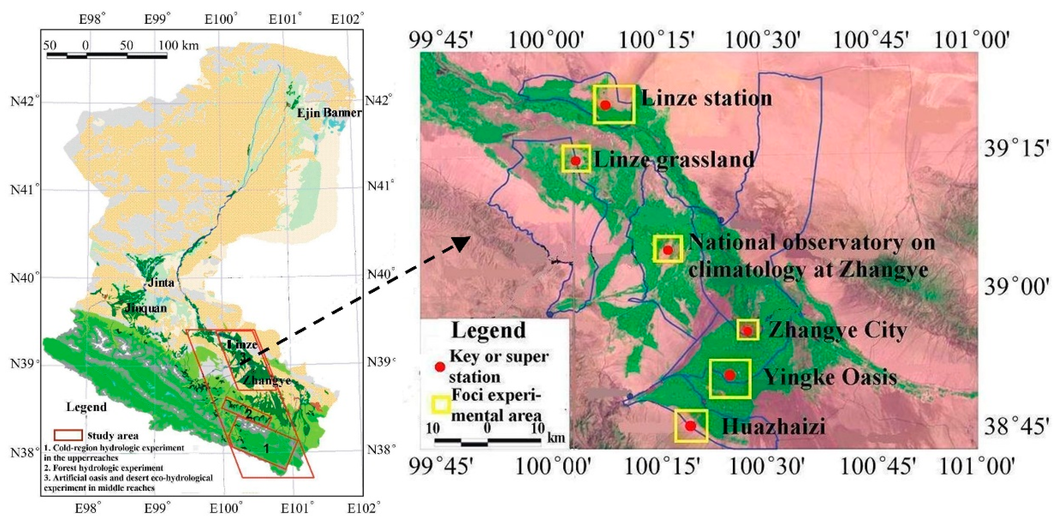
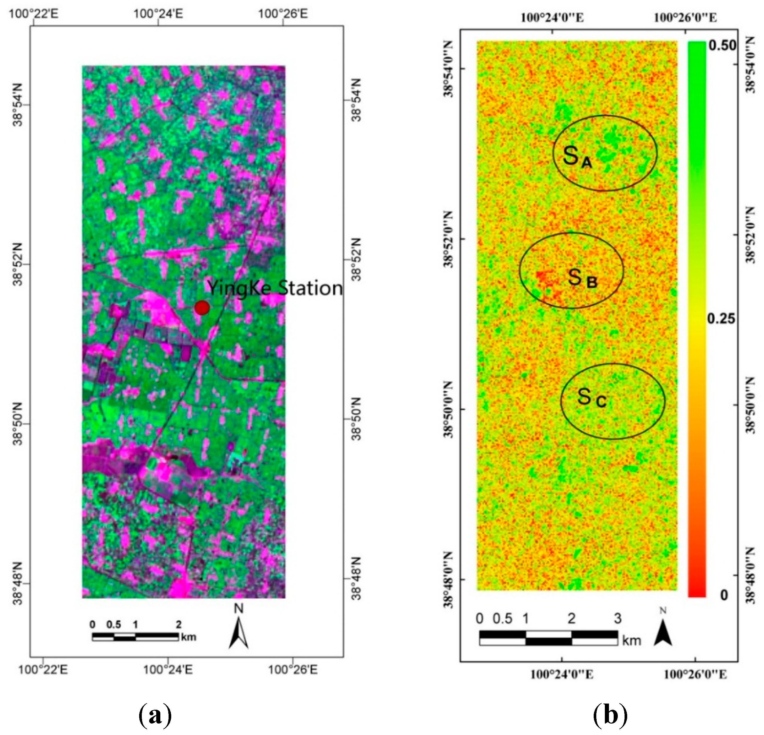
2.1. Study Area

Heihe River Basin is the second largest inland river basin in the arid region of northwest China. In the summer of 2008, an arid zone hydrology experiment was carried out in the Heihe River Basin [26,27]. The Yingke oasis foci experimental area was chosen as our study area (Figure 1). The experimental area belongs to an arid-emiarid, temperate continent climate. The mean annual precipitation is 121.5 mm and the annual mean air temperature is 6 °C. Total potential evaporation reaches 2340 mm per year—20 times more than the annual precipitation. Agriculture is typically referred to the oasis irrigated cultures, where corn (Zea mais, L.) and wheat (Triticum aestivum, L.) are the main plants in the area. The soil texture in study is homogeneous and composed by 16.7% sand, 74.8% silt, and 8.5% clay [21].
Figure 1. Heihe River Basin (left) and the locations of the Yingke oasis in the arid zone hydrology experiment area (right) (Referred to Li Xin et al. [26]).
Remotesensing 06 12055 g001

2.2. Satellite Data

The satellite data used in this study include Advanced Synthetic Aperture Radar (ASAR) dual-polarized data and Hyperion data. ASAR operates on the C band with a 5.6 cm wavelength. In this study, a VV/VH polarized Level 1B image (in the Alternating Polarization (AP) mode with a spatial resolution of 30 m) of the middle stream of the Heihe River Basin was selected. The image was captured on 11 July 2008 at 11:26. The Next ESA SAR Toolbox (NEST) was used to pre-process the data. NEST is an open source software, developed for ESA and made available via its website [28]. The Range-Doppler method was used to orthorectify the data with the SRTM 90 m void-filled Digital Elevation Model (DEM) downloaded from the Consortium for Spatial Information website [29,30]. Then, radiometric normalization and a 5 × 5 enhanced Lee filters was applied [31], and finally the backscatter values of study area were extracted. Hyperion has 242 bands with a spectrum ranging from 355 nm to 2577 nm, and the spatial resolution of Hyperion is 30 m [32,33]. The L1Gst data (Radiometrically corrected and resampled for geometric correction and registration to a geographic map projection. The data image is ortho-corrected using digital elevation models (DEM) to correct parallax error due to local topographic relief) in this paper was imaged on 15 July 2008. Atmospheric correction was made using the ENVI FLASSH (Fast Line-of-sight Atmospheric Analysis of Spectral Hypercubes) module [34,35]. The reflectance exhibited a high consistency when compared with the measured spectrum (determination coefficient more than 0.95) and met the requirements for retrieving vegetation biochemical parameters.

2.3. Field Data

From 13 June to 26 June 2008, measurements of the vegetation’s biochemical structure (namely: row spacing, leaf inclination angle, LAI, chlorophyll, canopy water content, and others are listed in the Branch and Leaf part of Table 1.) were conducted in the study area. In addition, on 29 June 2008, corn plants from every sample plot were taken back to the laboratory and dried to measure water content in the plant canopy. The water content of the corn canopy was obtained from 6 sample plots and ranged from 0.4 kg∙m−2 to 0.97 kg∙m−2 [36]. There were 16 days of delay between the remotely sensed observations and the canopy water content data. However, as the corn was at maturity, taking into account that no irrigation or rainfall occurred during this 16-day period, we have assumed that the water content changed little and that the fluctuation was acceptable [37]. Moreover, on 11 July 2008, soil moisture, from 12 cm deep in the Yingke 1–4 sample plots, was measured by time domain reflectometry (TDR) simultaneously with the ASAR transit over the study area. In each sample plot, soil moisture was measured three times and at last we get the mean values of the measurements. All the sample plots are representative.
Table 1. Input Parameters of michigan microwave canopy scattering (MIMICS).
TypeMIMICS Model Input ParametersRange
Soil surfaceSoil moisture0.2 cm3∙cm−3
Surface correlation length12 cm
RMS height1 cm
Surface temperature24°
Soil sand16.7%
Soil clay8.5%
BranchBranch length1.17 m
Branch diameter2.9 cm
Branch weight water0.6
Branch dry matter density0.1 g∙cm−2
Branch density15.0 N∙m−3
leafLeaf weight water0.78
Leaf dry matter density0.005 g·cm−2
Leaf thickness0.024 cm
Leaf width6 cm
Leaf length60 cm
Leaf diameter9 cm
Leaf density20, 30, ..., 400 N∙m3
Leaf angle distributionPlagiophile
SensorAngle of incidence31.5°
Frequency1.4, 3.0, 5.33 GHz

3. Methodology

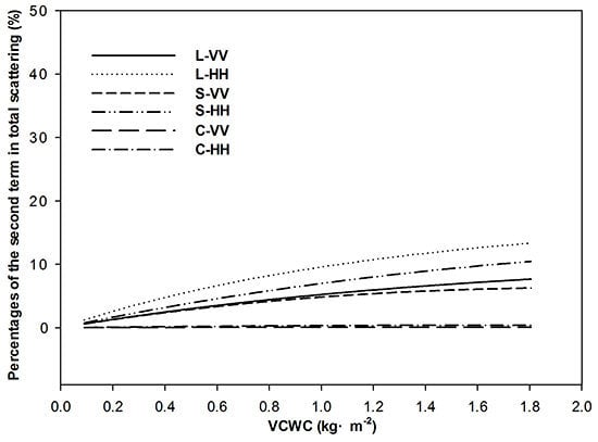
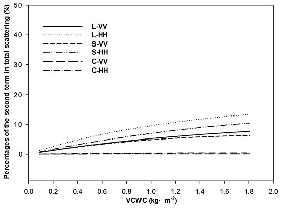
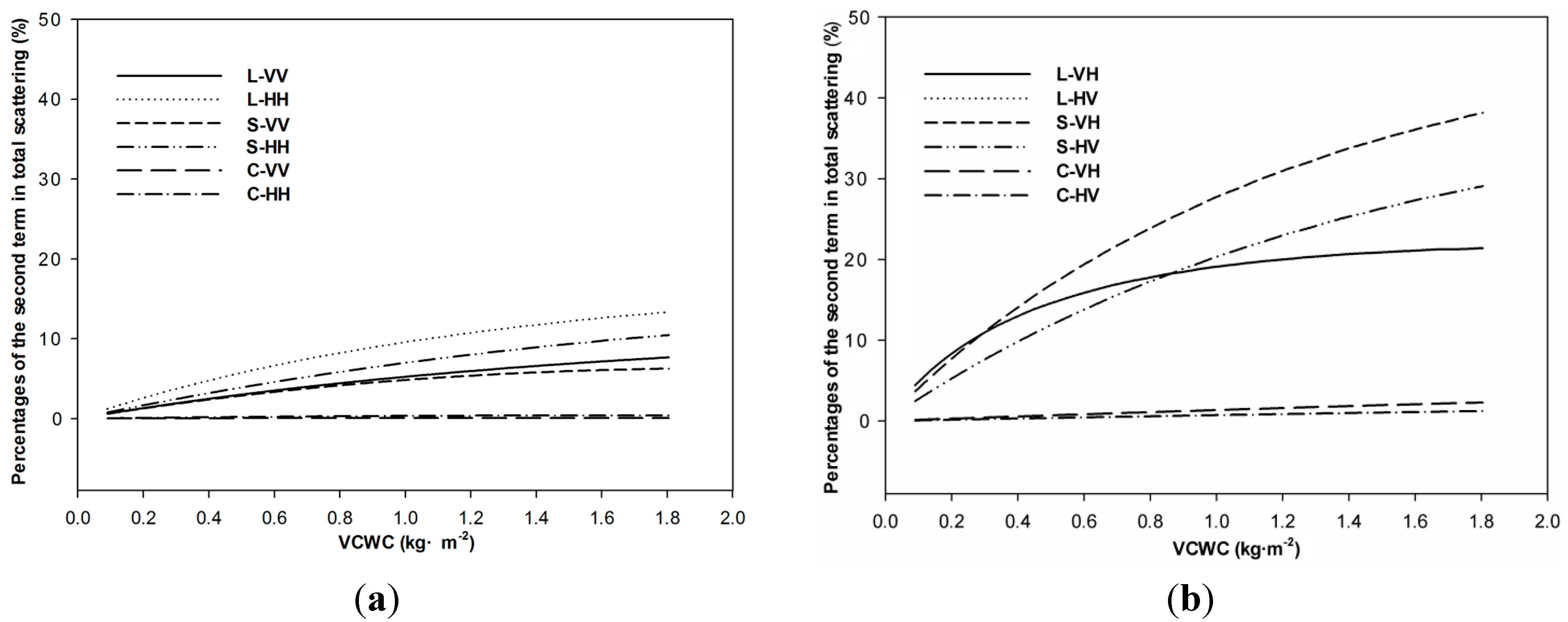
3.1. Scattering Characteristics in Agricultural Regions

For agricultural regions, tree trunk scattering in the MIMICS model can be ignored [38]. In addition, the third term scattering (i.e., ground-canopy-ground interaction) can also be ignored because it contributes little to the total scattering [39]. Distinct from these two, the calculated percentages for the second term scattering (i.e., crown ground interaction) in total scattering varies from study to study due to the diverse study methods [40,41]. Using the data in Table 1 as the input parameters, we simulated features of vegetation backscattering and calculated the percentages of the second term in total scattering under different frequency and canopy water contents.
Figure 2 uses corn as the research subject and simulates the percentages of the second term scattering in total scattering under different polarizations and wavelengths. Figure 2 shows that the percentages of the second term scattering, in different polarizations and wavelengths, gradually increased with increasing canopy water content. For band L, second term scattering possesses some percentage under four polarizations. Cross-polarization has at most 20%, while co-polarizations possess at most 15%. HH polarization possesses a higher percentage compared with VV. For band S, second term scattering possesses some percentages under four polarizations as well. VH has at most 40%, while HV possesses at most 30%. In general, co-polarization is at most 10%. For band C, second term scattering from four polarizations account for little in total scattering. VH possesses at most 2% and HV accounts for 1.2%. The second term scattering from co-polarization, VV and HH, are both less than 1%. For SAR band L and band S data, ignoring the second term scattering for the crown-ground interaction cannot be adopted simply when taking into account the vegetation scattering. However, for band C, especially for co-polarization data, the crown-ground interaction can be ignored.
Figure 2. Percentage of the second term scattering with different bands and different polarization in total scattering (L, S, C represent the different bands, and VV, HH, VH, and HV represent the different polarizations). (a) Co-polarization (Plots from top to bottom are L-HH, S-HH, L-VV, S-VV, C-HH, C-VV); (b) Cross-polarization (Plots from top to bottom are S-VH, S-HV, (L-VH, L-HV), C-VH, C-HV).
Remotesensing 06 12055 g002

3.2. Scattering Model in Agricultural Regions

Considering the theories mentioned above, we improved the Water-Cloud model by adding the second term for crown-ground interactions and address the canopy layer as a single layer in crop areas. The total backscattering σ p q   0 consists of three parts: the direct reflection by vegetation backscattering σ p q 1 0 , the second term scattering for the crown-ground interaction σ p q 2 0 and σ p q 3 0 , and the direct reflection decayed by the land surface [41]:
σ p q 0 = σ p q 1 0 + σ p q 2 0 + σ p q 3 0 = A m v e g cos (θ) (1- L p q 2 ) +2 C ( R p + R q ) L p q 2 + σ soil 0 L p q 2
where p is polarization of transmission; q is polarization of reception; R p   and R q are Fresnel reflection coefficients; L p q 2 = exp ( θ 2 B m v e g sec ( θ ) ) is a two-way extinction coefficient and σ s o i l 0 is soil direct backscattering calculated by a simplified model [42], m v e g is the vegetation canopy water content. The final expression of the model is as follows:
σ p q 0 = σ p q 1 0 + σ p q 2 0 + σ p q 3 0 = A m v e g cos (θ) (1 - exp( - 2 B m v e g sec(θ ) ) ) + 2C( R p + R q )exp(-2 B m v e g sec(θ ) ) + 10 [ D v v ( θ ) log 10 ( M v ) + E v v ( θ ) log 10 ( Z s ) + F v v ( θ ) ] / 10 exp(-2 B m v e g sec(θ ) )         
In the model, A, B and C are parameters dependent on the types of vegetation, the frequency, and the polarization, which can be simulated by the MIMICS model, m v e g   can be calculated by optical data. Soil moisture retrieval model can be established using dual-polarized data by combining the model in different polarization.

3.3. Calculation of Vegetation Canopy Water Content

PROSAIL is a combination of the PROSPECT leaf RT model and the SAIL canopy RT model [43,44,45], which has been used extensively for a variety of applications [46]. At the leaf level, PROSAIL uses leaf chlorophyll content (Cab), equivalent leaf water thickness (EWT), leaf structure parameter (N) and leaf dry matter (Cm) as inputs. At the canopy level, input parameters are LAI, leaf inclination angle distribution, soil brightness, ratio diffuse/direct irradiation, solar zenith angle, view zenith angle and Sun-view azimuth angle [47]. Based on this, we tried to obtain vegetation canopy water content using Hyperion data based on the PROSAIL and then calculated the contribution provided by the vegetation layer to backscattering.
There is a leaf water absorption band centered on 970 m, which results in the first-order derivative of the absorption curve being related to the canopy water content [47,48,49]. In addition, the Hyperion sensor can only provide hyperspectral data with a resolution of 10 nm, resulting in the failure of obtaining a more accurate spectral first-order derivative (1 nm level). Vegetation canopy water content index Derivative 980–1070 nm (D980–1070) can be used to retrieve vegetation canopy water content and can eliminate the influence of spectral resolution and imaging noises, making the results more precise. According to related research, the linear model of D980–1080 and m v e g   was established as follows [50]:
m v e g = 0.2912 D 980 1070 0.4693

4. Results and Analysis

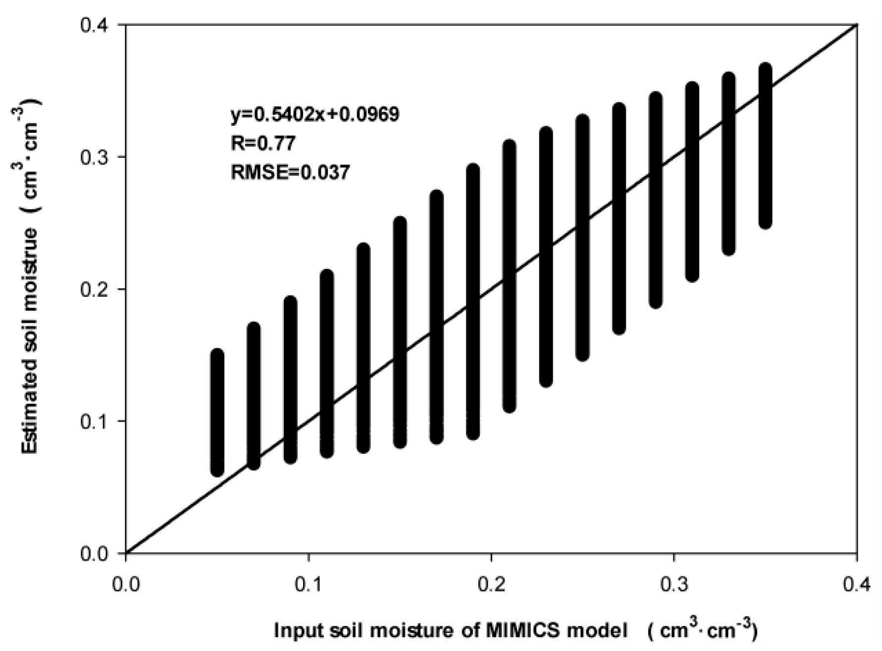
4.1. Soil Moisture Retrieval Model

The ASAR data acquired in this study are in the C band and are polarized in the VV/VH mode. Accordingly, the second term scattering is ignored. The percentage of the second term scattering is low, especially for VV polarization (only 0.2%). According to Equation (2) and the coefficients A and B in the VV and VH polarization calculated from the MIMICS model, the following parameters can be obtained:
A v v = 0.0968 m v e g 1 B v v = 0.4170 A v h = 0.0002 m v e g 1 B v h = 0.389
Combining the algorithms above, the retrieval model of soil moisture can be obtained:
M v = 10 G v v v h ( θ ) σ v v _ s o i l + H v v v h ( θ ) σ v h _ s o i l + I v v v h ( θ ) σ v v _ s o i l = ( σ v v 0 A v v m v e g cos (θ) (1- L v v 2 ) / L v v 2 σ v h _ s o i l = ( σ v h 0 A v h m v e g cos (θ) (1- L v h 2 ) / L v h 2 G v v v h ( θ ) = 0.3802 cos 2 ( θ ) 0.6043 cos ( θ ) + 0.2354 H v v v h ( θ ) = 1.7827 cos 2 ( θ ) 2.8678 cos ( θ ) + 1.1879 I v v v h ( θ ) = 34.087 cos 2 ( θ ) 54.922 cos ( θ ) + 22.279 L v v 2 = exp(-2 B v v m v e g sec(θ ) ) ) L v h 2 = exp(-2 B v h m v e g sec(θ ) ) )
where m v e g   is retrieved from Hyperion data and θ   can be read from the SAR image. Using the ASAR dual-polarized data, we removed combination roughness to acquire retrieved soil moisture. Thus, the retrieval model of soil moisture in vegetated areas, based on SAR and hyperspectral data, has been established. The scattering of VV and VH in C band on vegetated areas can be simulated according Table 1 (Frequency was fixed in 5.33 GHz). There are 37,440 pairs of simulated data in total, representing all types of land surfaces in the study area. According to model (5), soil moisture can be retrieved.
Figure 3 indicates that soil moisture from the retrieval model is well correlated with soil moisture from the MIMICS model. The correlation coefficient is 0.77 with a root mean square error of 0.037 cm3∙cm−3. This correlation coefficient indicates that the proposed soil moisture retrieval model is feasible.
Figure 3. Comparison between retrieval results from model (5) and soil moisture imported to the MIMICS model.
Remotesensing 06 12055 g003

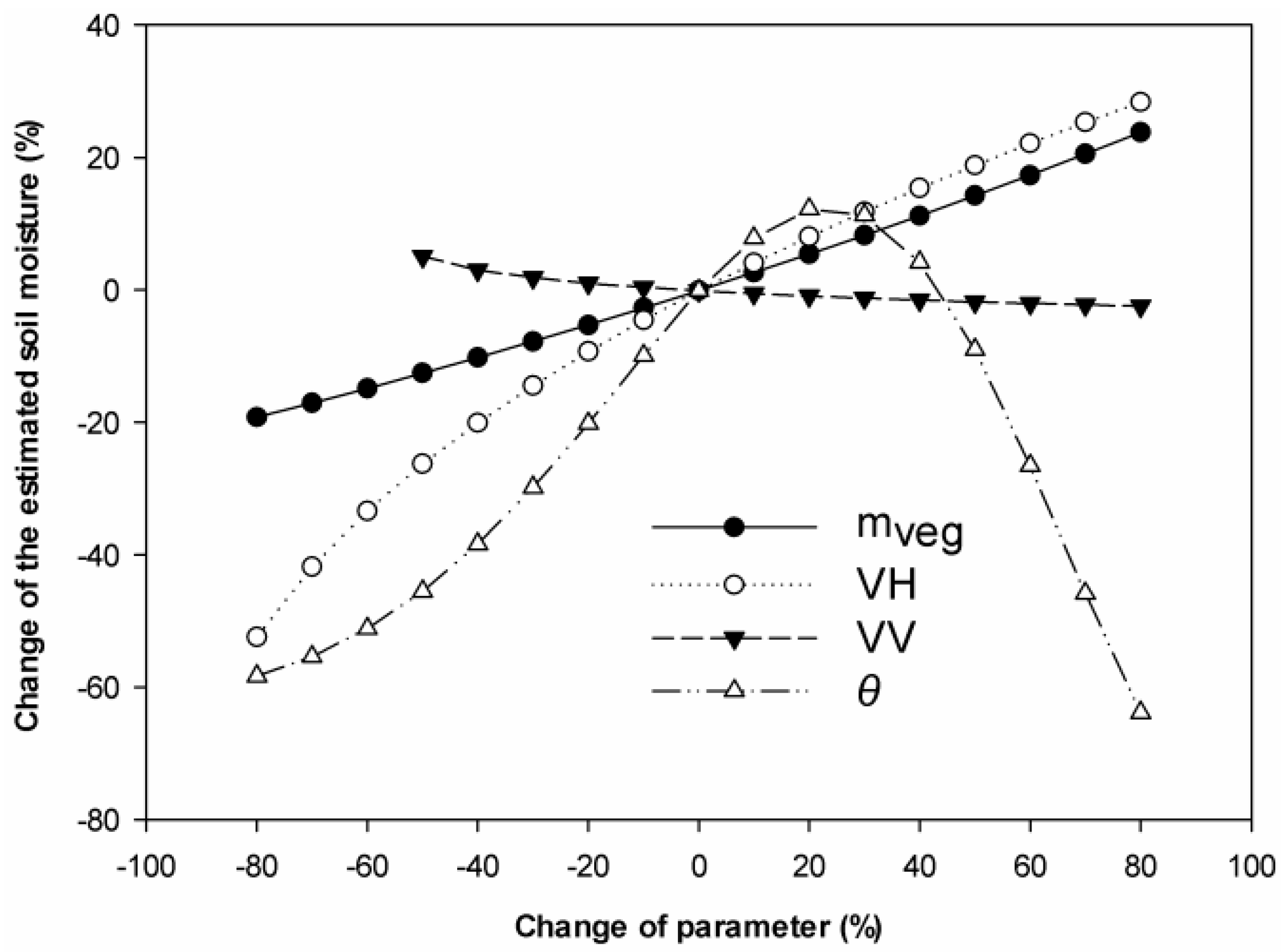
4.2. Sensitivity Analysis

The sensitivity of parameters in the model was analyzed (see Figure 4). It can be concluded that the model shows sensitivity towards angle, canopy water content and backscattering in VH polarization. With increased angles, the retrieved soil moisture initially increased and then subsequently decreased. With increasing canopy water content and VH polarized backscattering, the soil moisture is increasing. It indicated from Figure 3 that the result error of canopy water inversion would lead to 5% retrieval error of soil moisture. For backscattering of VV polarization, the model shows low sensitivity.
Figure 4. The analysis of sensitivity of parameters in model (5).
Remotesensing 06 12055 g004

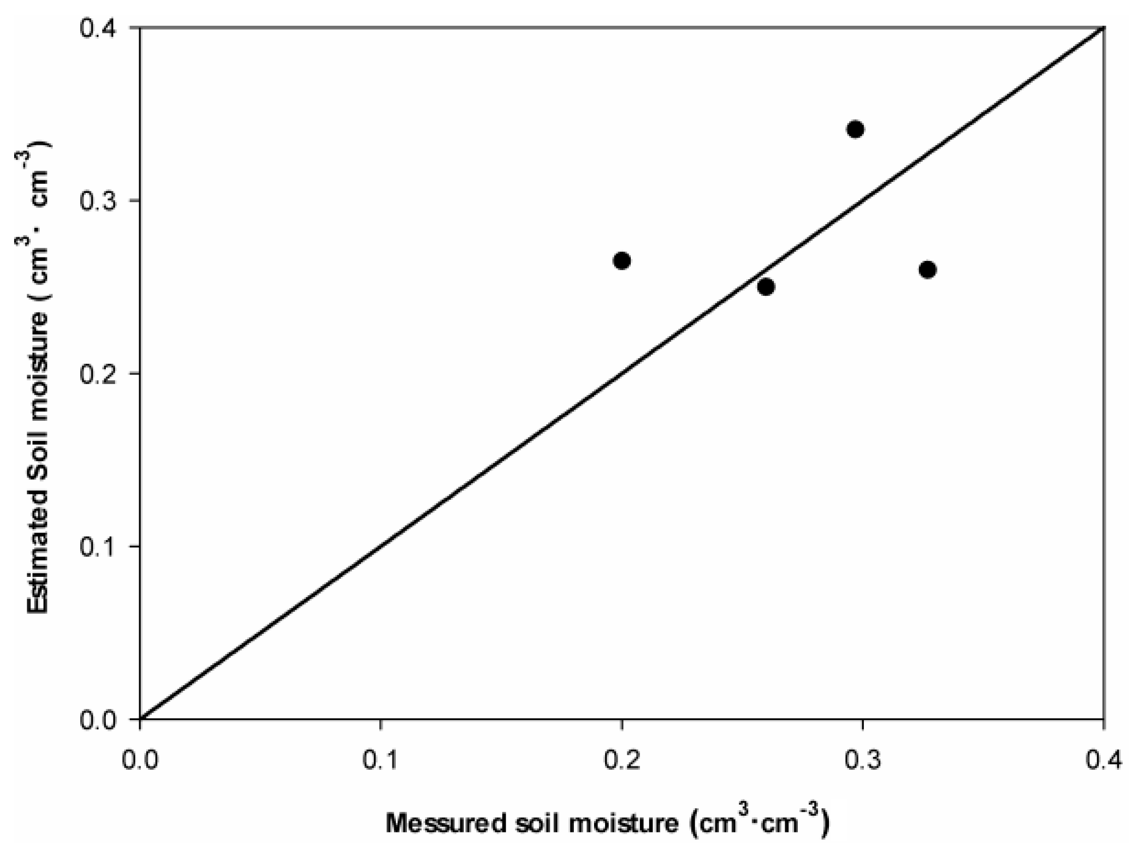
4.3. Soil Moisture Estimation

Firstly, the paper chose 9 spectral data from Hyperion to calculate D980–1070 and the central wavelengths from the data are 983,993, 1003, 1023, 1033, 1043, 1053, and 1063 nm. Retrieving the vegetation canopy water content in Yingke oasis region can be accomplished using Equation (3). Result indicated that RMSE was within 0.1 kg∙m−2, AARD was 12.5%, and the proposed model was practical and reliable. Then, using the model mentioned in Equation (5), we can estimate the soil moisture in the Yingke oasis. The retrieved result is displayed in Figure 5b. From the figure, it can be concluded that the spatial differences in soil moisture is evident. Some regions have higher soil water content (i.e., SA area), while the values in other regions appear to be lower (i.e., SB area). While the regions with the lower soil moisture values (i.e., SB area) had low vegetation coverage and a greater number of villages (Figure 5a). The soil moisture in most regions (i.e., SC area) ranged from 0.20 cm3∙cm−3 up to 0.35 cm3∙cm−3, which is sufficient to satisfy the needs of crop growth. The overall estimate of soil moisture is reasonable in spatial distribution.
On 11 July 2008, soil moisture from 12 cm deep in the Yingke 1–4 sample plots was measured simultaneously with the ASAR transit over the study area. The study uses these four points as experimental data to confirm the retrieved results, as shown in Figure 6. It can be observed that there is a significant linear relationship between the soil moisture derived from the estimation and the actual measurement results. Due to few data points, our research just calculated the absolute and relative error. The average absolute deviation (AAD) was 0.051 cm3∙cm−3, average absolute relative deviation of these four points is 19.7% (Figure 6). Besides, we calculated TVDI using MODIS data in the same day of measured data. Soil moisture data was resampled in 1km and compared with TVDI (see Figure 7). It showed good relationship between soil moisture and TVDI (R = 0.65). These indicated the reliability and applicability of the model proposed in this study.
Figure 5. Hyperion image in RGB color (a) and retrieval image of soil moisture (cm3∙cm−3) in study area (b).
Remotesensing 06 12055 g005
Figure 6. Comparison between soil moisture from the retrieval model and the measurements in the Yingke oasis area.
Remotesensing 06 12055 g006
Figure 7. Comparison between estimated soil moisture and MODIS-derived TVDI.
Remotesensing 06 12055 g007

5. Conclusions

In this study, a new approach was introduced to estimate surface soil moisture in vegetated areas. The soil moisture retrieval model for vegetated regions was developed by combining microwave and hyperspectral remote sensing. The percentages of second term scattering (i.e., crown ground interaction) in total scattering of different bands were discussed in detail. For band L, Cross-polarization has at most 20%, while co-polarizations possess at least 10%. For band S, VH has at most 40%, while HV possesses at most 30%. In general, co-polarization is at most 10%. For band C, second term scattering from four polarizations account for little in total scattering (no more than 3%). Hence, for SAR band L and band S data, ignoring the second term scattering cannot be adopted simply when taking into account the vegetation scattering. However, for band C, the crown-ground interaction can be ignored.
VCWC, one important parameter of the retrieval model, was obtained using a vegetation canopy water content index D980–1070 based on Hyperion data, and satisfactory result was achieved. It implies that hyperspectral data has an advantage of VCWC retrieval than multi-spectral remote sensing data, and more hyperspectral data should been used in the soil moisture inversion.
Alternating polarization data of ASAR and Hyperion hyperspectral data were used to measure soil moisture and to confirm the feasibility of the retrieval model. The results showed that the proposed model was suitable for vegetated areas. Generally, the accuracy of the model (AAD was 0.051 cm3∙cm−3, AARD was 19.7%) meets the demand for the soil moisture retrieval of vegetated areas at a regional scale. Future works should use more field measurements to validate the method and extend the application of the proposed method over other study regions.

Acknowledgments

This work was supported by the CAS Action Plan for West Development Program under Grant KZCX2-XB3-15 and National Natural Science Foundation of China under Grant 41271379. The authors are indebted to the Cold and Arid Regions Science Data Center for providing the ASAR data and ground data that were used in this manuscript. Thanks are also given to the Geospatial Data Cloud for providing the Hyperion data.

Author Contributions

Xiaoning Song drafted the manuscript and was responsible for the research design, experiment and analysis. Jianwei Ma reviewed the manuscript and was responsible for the research design and analysis. Pei Leng and Xiaotao Li supported the data preparation and the interpretation of the results. Fangcheng Zhou and Shuang Li provided some of the data and gave relevant technical support. All of the authors contributed to editing and reviewing the manuscript.

Conflicts of Interest

The authors declare no conflict of interest.

References

  1. Baghdadi, N.; Holah, N.; Zribi, M. Soil moisture estimation using multi-incidence and multi-polarization ASAR data. Int. J. Remote Sens. 2006, 10, 1907–1920. [Google Scholar] [CrossRef]
  2. Baghdadi, N.; Zribi, M. Evaluation of radar backscatter models IEM, OH and Dubois using experimental observations. Int. J. Remote Sens. 2006, 27, 3831–3852. [Google Scholar] [CrossRef]
  3. Wagner, W.; Lemoine, G.; Rott, H. A method for estimating soil moisture from ERS scatterometer and soil data. Remote Sens. Environ. 1999, 70, 191–207. [Google Scholar] [CrossRef]
  4. Baudena, M.; Bevilacqua, I.; Canone, D.; Ferraris, S.; Previati, M.; Provenzale, A. Soil water dynamics at a midlatitude test site: Field measurements and box modeling approaches. J. Hydrol. 2012, 414–415, 329–340. [Google Scholar] [CrossRef]
  5. Kornelsen, K.C.; Coulibaly, P. Advances in soil moisture retrieval from synthetic aperture radar and hydrological applications. J. Hydrol. 2013, 476, 460–489. [Google Scholar] [CrossRef]
  6. Seneviratne, S.I.; Corti, T.; Davin, E.L.; Hirschi, M.; Jaeger, E.B.; Lehner, I.; Orlowski, B.; Teuling, A.J. Investigating soil moisture-climate interactions in a changing climate: A review. Earth-Sci. Rev. 2010, 99, 125–161. [Google Scholar]
  7. Brocca, L.; Tarpanelli, A.; Melone, F.; Moramarco, T.; Caudaro, M.; Ratto, S.; Ferraris, S.; Berni, N.; Ponziani, F.; Wagner, W.; et al. Soil moisture estimation in alpine catchments through modelling and satellite observations. Vadose Zone J. 2013, 12. [Google Scholar] [CrossRef]
  8. Zribi, M.; Baghdadi, N.; Guerin, C. Analysis of surface roughness heterogeneity and scattering behavior for radar measurements. IEEE Trans. Geosci. Remote Sens. 2006, 44, 2438–2444. [Google Scholar] [CrossRef]
  9. Wang, S.G.; Li, X.; Han, X.J.; Jin, R. Estimation of surface soil moisture and roughness from multi-angular ASAR imagery in the watershed allied telemetry experimental research (WATER). Hydrol. Earth Syst. Sci. 2011, 15, 1415–1426. [Google Scholar] [CrossRef]
  10. Dobson, M.C.; Ulaby, F.T.; Hallikainen, M.T.; Elrayes, M.A. Microwave dielectric behavior of wet soil 2: Dielectric mixing models. IEEE Trans. Geosci. Remote Sens. 1985, 23, 35–46. [Google Scholar]
  11. Oh, Y.; Sarabandi, K.; Ulaby, F.T. An empirical model and an inversion technique for radar scattering from bare soil surfaces. IEEE Trans. Geosci. Remote Sens. 1992, 30, 370–381. [Google Scholar] [CrossRef]
  12. Svoray, T.; Shoshany, M. Multi-scale analysis of intrinsic soil factors from SAR-based mapping of drying rates. Remote Sens. Environ. 2004, 92, 233–246. [Google Scholar] [CrossRef]
  13. Zribi, M.; Saux-Picart, S.; Andre, C.; Descroix, L.; Ottle, C.; Kallel, A. Soil moisture mapping based on ASAR/ENVISAT radar data over a Sahelian region. Int. J. Remote Sens. 2007, 28, 3547–3565. [Google Scholar] [CrossRef]
  14. Merzouki, A.; McNairn, H.; Pacheco, A. Mapping soil moisture using RADARSAT-2 data and local autocorrelation statistics. IEEE J. Sel. Top. Appl. Earth Obs. Remote Sens. 2011, 4, 128–137. [Google Scholar] [CrossRef]
  15. Lievens, H.; Verhoest, N.E.C. Spatial and temporal soil moisture estimation from RADARSAT-2 imagery over Flevoland, The Netherlands. J. Hydrol. 2012, s456–s457, 44–56. [Google Scholar] [CrossRef]
  16. Liu, W. Study on Soil Moisture Inversion and Application with Polarization Radar in Vegetated Area. Ph.D. Thesis, Chinese Academy of Science, Beijing, China, 2005. [Google Scholar]
  17. Attema, E.P.W.; Ulaby, F.T. Vegetation modeled as a water cloud. Radio Sci. 1978, 13, 357–364. [Google Scholar] [CrossRef]
  18. Ulaby, F.T.; Sarabandi, K.; McDonald, K.; Whitt, M.; Dobson, M.C. Michigan microwave canopy scattering model. Int. J. Remote Sens. 1990, 11, 1223–1253. [Google Scholar] [CrossRef]
  19. Zhou, P.; Ding, J.L.; Wang, F.; Guljamal, U.; Zhang, Z.G. Retrieval methods of soil water content in vegetation covering areas based on multi-source remote sensing data. J. Remote Sens. 2010, 14, 966–972. (In Chinese) [Google Scholar]
  20. Wang, C.; Qi, J.; Moran, S.; Marsett, R. Soil moisture estimation in a semiarid rangeland using ERS-2 and TM imagery. Remote Sens. Environ. 2004, 90, 178–189. [Google Scholar] [CrossRef]
  21. Yu, F.; Zhao, Y.S. A new semi-empirical model for soil moisture content retrieval by ASAR and TM data in vegetation-covered areas. Sci. China: Earth Sci. 2011, 41, 532–540. (In Chinese) [Google Scholar]
  22. Saradjian, M.R.; Hosseini, M. Soil moisture estimation by using multipolarization SAR image. Adv. Space Res. 2011, 2, 278–286. [Google Scholar] [CrossRef]
  23. Cheng, Y.B.; Zarco-Tejada, P.J.; Riaño, D.; Rueda, C.A.; Ustin, S.L. Estimating vegetation water content with hyperspectral data for different canopy scenarios: Relationships between AVIRIS and MODIS indexes. Remote Sens. Environ. 2006, 105, 354–366. [Google Scholar] [CrossRef]
  24. Fung, A.K.; Li, Z.; Chen, K.S. Backscattering from a randomly rough dielectric surface. IEEE Trans. Geosci. Remote Sens. 1992, 30, 356–369. [Google Scholar] [CrossRef]
  25. Wu, T.D.; Chen, K.S. A reappraisal of the validity of the IEM model for backscattering from rough surface. IEEE Trans. Geosci. Remote Sens. 2004, 42, 743–753. [Google Scholar] [CrossRef]
  26. Li, X.; Li, X.W.; Li, Z.Y.; Ma, M.G.; Wang, J.; Xiao, Q. Watershed allied telemetry experimental research. J. Geophys. Res. 2009, D22103, 1–19. [Google Scholar]
  27. Li, X.; Li, X.W.; Roth, K.; Menenti, M.; Wagner, W. Preface “observing and modeling the catchment scale water cycle”. Hydrol. Earth Syst. Sci. 2011, 2, 597–601. [Google Scholar] [CrossRef]
  28. NEST. Next ESA SAR toolbox Website. European Space Agency 2013. Available online: http://nest.array.ca/web/nest (accessed on 20 May 2014).
  29. Small, D.; Schubert, A. Guide to ASAR Geocoding; RSL-ASAR-GC-AD (1.01). University of Zürich: Zürich, Switzerland, 2008. Available online: http://www.geo.unizh.ch/microsite/rsl-documents/research/publications/other-sci-communications/2008_RSL-ASAR-GC-AD-v101-0335607552/2008_RSL-ASAR-GC-AD-v101.pdf (accessed on 20 May 2014).
  30. Jarvis, A.; Reuter, H.; Nelson, A.; Guevara, E. Hole-filled SRTM for the Globe Version 4, Available from the CGIAR-CSI SRTM 90 m Database 2008. Available online: http://srtm.csi.cgiar.org (accessed on 22 May 2014).
  31. Kellndorfer, J.M.; Pierce, L.E.; Dobson, M.C.; Member, S.; Ulaby, F.T. Toward consistent regional-to-global-scale vegetation characterization using orbital SAR systems. IEEE Trans. Geosci. Remote Sens. 1998, 36, 1396–1411. [Google Scholar] [CrossRef]
  32. Pearlman, J.S.; Barry, P.S.; Segal, C.C.; Shepanski, J.; Beiso, D.; Carman, S.L. Hyperion, a space-based imaging spectrometer. IEEE Trans. Geosci. Remote Sens. 2003, 41, 1160–1173. [Google Scholar] [CrossRef]
  33. Ungar, S.G.; Pearlman, J.S.; Mendenhall, J.A.; Reuter, D. Overview of the Earth Observing One (EO-1) mission. IEEE Trans. Geosci. Remote Sens. 2003, 41, 1149–1159. [Google Scholar] [CrossRef]
  34. Jafari, R.; Lewisb, M.M. Arid land characterisation with EO-1 Hyperion hyperspectral data. IEEE J. Sel. Top. Appl. Earth Obs. Remote Sens. 2012, 19, 298–307. [Google Scholar]
  35. Yuan, J.G.; Niu, Z.; Wang, X.P. Atmospheric correction of Hyperion hyperspectral image based on FLAASH. Spectrosc. Spectr. Anal. 2009, 29, 1181–1185. (In Chinese) [Google Scholar]
  36. Wu, C.Y.; Gao, S.; Dong, J.J. WATER: Dataset of Crop Biochemical Parameter Measurements in the Yingke Oasis Foci Experimental Area. Available online: http://westdc.westgis.ac.cn/data/e347aef0-5c3b-40cd-9a08-7c0e89470898 (accessed on 12 October 2012).
  37. Zhu, X.H.; Feng, X.M.; Zhao, Y.S.; Song, X.N. Scale effect and error analysis of crop LAI inversion. J. Remote Sens. 2010, 14, 586–592. (In Chinese) [Google Scholar]
  38. De Roo, R.D.; Du, Y.; Ulaby, F.T.; Dobson, M.C. A semi-empirical backscattering model at L-band and C-band for a soybean canopy with soil moisture inversion. IEEE Trans. Geosci. Remote Sens. 2001, 39, 864–872. [Google Scholar] [CrossRef]
  39. Bao, Y.S.; Liu, L.; Wang, J.H. Soil moisture estimation based on optical and microwave remote sensing data. J. Beijing Norm. Univ. Nat. Sci. 2007, 43, 228–233. (In Chinese) [Google Scholar]
  40. Shi, J.C.; Li, Z.; Li, X.W. Evaluate usage of decomposition technique in estimation of soil moisture with vegetated surface by multi-temporal measurements data. J. Remote Sens. 2002, 6, 412–415. (In Chinese) [Google Scholar]
  41. Liu, W.; Shi, J.C. Applying the radar technology to estimate relative change of soil moisture in vegetated area. Adv. Water Sci. 2005, 16, 596–601. (In Chinese) [Google Scholar]
  42. Ma, J.W.; Song, X.N.; Li, X.T.; Leng, P.; Li, S.; Zhou, F.C. Estimation of surface soil moisture from ASAR dual-polarized data in the middle stream of the Heihe River Basin. Wuhan Univ. J. Nat. Sci. 2013, 02, 163–170. [Google Scholar] [CrossRef]
  43. Verhoef, W. Light scattering by leaf layers with application to canopy reflectance modeling: The SAIL model. Remote Sens. Environ. 1984, 16, 125–141. [Google Scholar] [CrossRef]
  44. Jacquemoud, S.; Baret, F. Prospect-a model of leaf optical properties spectra. Remote Sens. Environ. 1990, 34, 75–91. [Google Scholar] [CrossRef]
  45. Jacquemoud, S.; Baret, F.; Andrieu, B.; Danson, F.M.; Jaggard, K. Extraction of vegetation biophysical parameters by inversion of the PROSPECT+SAIL models on sugar beet canopy reflectance data-Application to TM and AVIRIS sensors. Remote Sens. Environ. 1995, 52, 163–172. [Google Scholar] [CrossRef]
  46. Jacquemoud, S.; Verhoef, W.; Baret, F.; Bacour, C.; Zarco-Tejada, P.J.; Asner, G.P.; Francois, C.; Ustin, S.L. PROSPECT+SAIL models: A review of use for vegetation characterization. Remote Sens. Environ. 2009, 113, S56–S66. [Google Scholar] [CrossRef]
  47. Clevers, J.G.P.W.; Kooistra, L.; Schaepman, M.E. Estimating canopy water content using hyperspectral remote sensing data. IEEE J. Sel. Top. Appl. Earth Obs. 2010, 12, 119–125. [Google Scholar] [CrossRef]
  48. Penuelas, J.; Filella, I.; Biel, C.; Serrano, L.; Save, R. The reflectance at the 950–970 mm region as an indicator of plant water status. Int. J. Remote. Sens. 1993, 14, 1887–1905. [Google Scholar] [CrossRef]
  49. Tucker, C.J. Remote sensing of leaf water content in the near infrared. Remote Sens. Environ. 1980, 10, 23–32. [Google Scholar] [CrossRef]
  50. Song, X.N.; Ma, J.W.; Li, X.T.; Leng, P.; Zhou, F.C.; Li, S. Estimation of vegetation canopy water content using Hyperion hyperspectral data. Spectrosc. Spectr. Anal. 2013, 10, 2833–2837. (In Chinese) [Google Scholar]

