Canopy Height Estimation in French Guiana with LiDAR ICESat/GLAS Data Using Principal Component Analysis and Random Forest Regressions

 , , ,
, , ,
Abstract
:
1. Introduction
2. Dataset Description
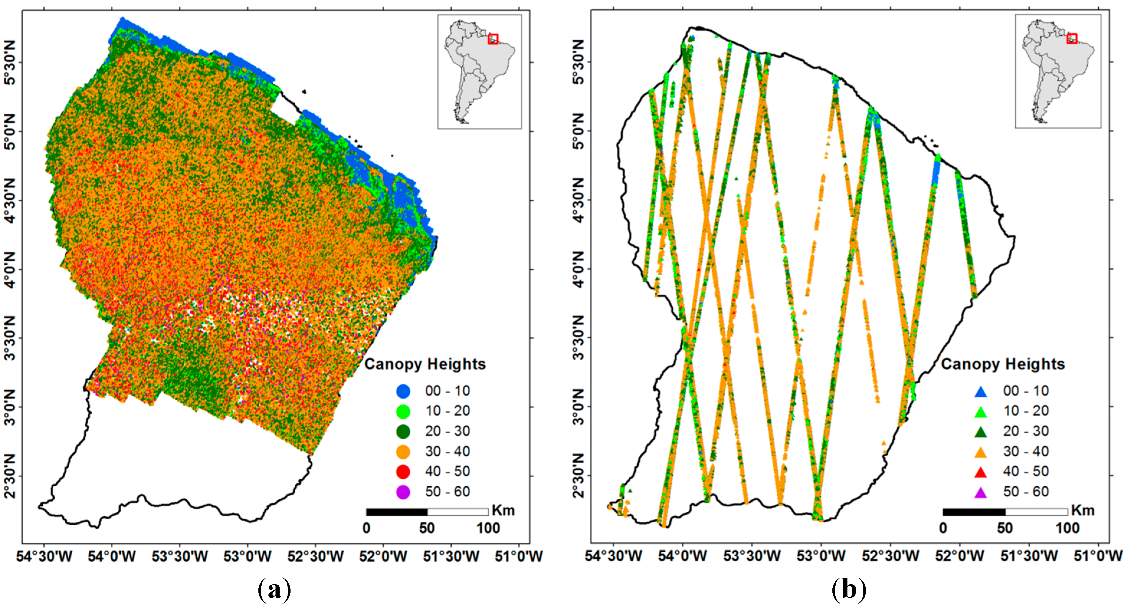
2.1. Study Area
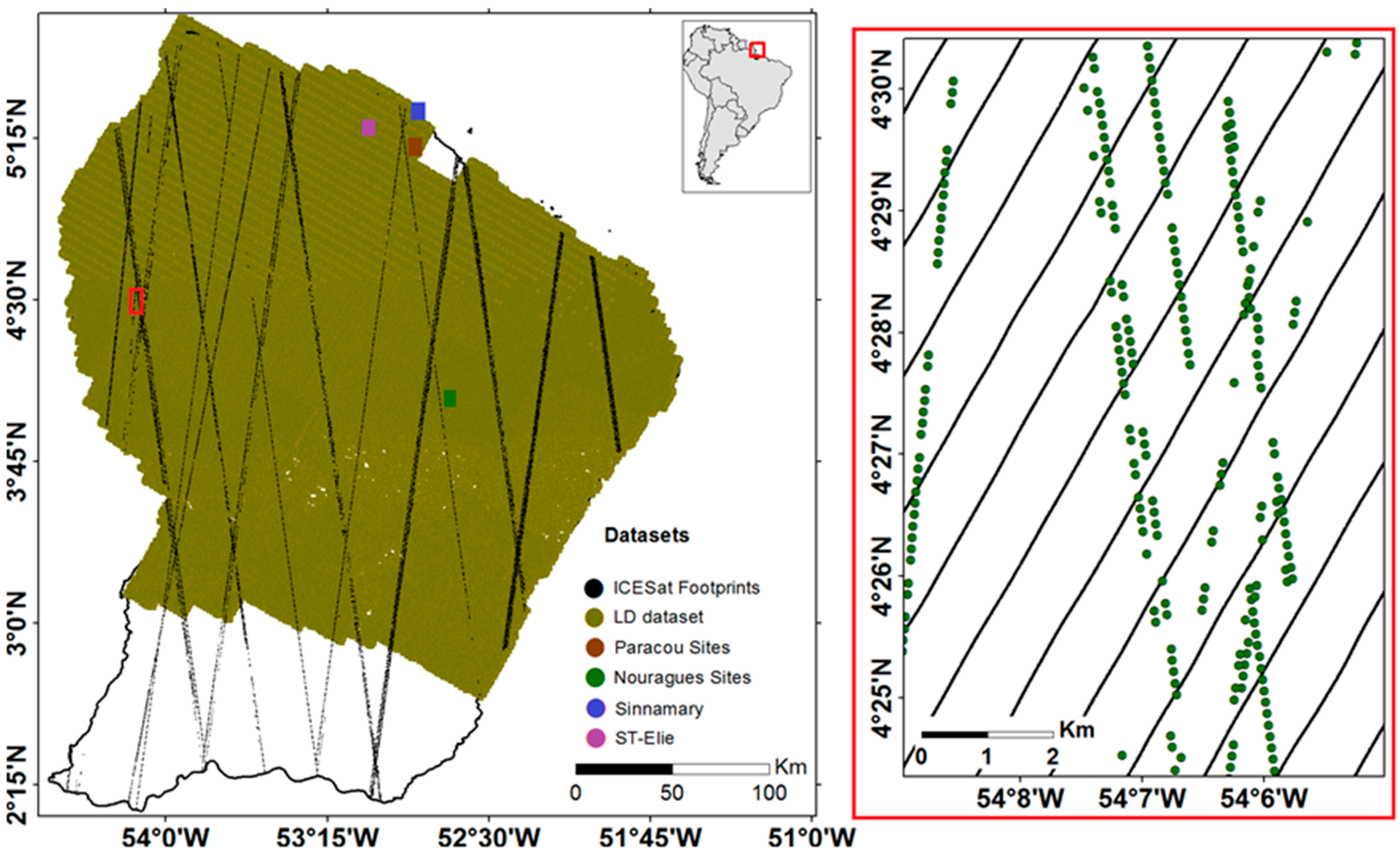
2.2. Airborne LiDAR Dataset
2.2.1. Small-Footprint Low-Density LiDAR Dataset (LD)
2.2.2. Small-Footprint High-Density LiDAR Dataset (HD)

| Site | Acquisition Date | Location | Area (km2) | Point Density (points/m2) |
|---|---|---|---|---|
| Paracou_2004 | 2004 | 5°15.9ʹN 52°55.9ʹW | 5.35 | 0.9 |
| Sinnamary | 2004 | 5°24.7ʹN 52°56ʹW | 6.52 | 0.9 |
| St-Elie | 2007 | 5°18.2ʹN 53°3.3ʹW | 4.40 | 5.3 |
| Nouragues07A | 2007 | 4°5.3ʹN 52°40.7ʹW | 7.24 | 3.2 |
| Nouragues07B | 2007 | 4°2.4ʹN 52°40.6ʹW | 2.42 | 3.8 |
| Nouragues08A | 2008 | 4°5.1ʹN 52°41.2ʹW | 1.96 | 4.5 |
| Nouragues08B | 2008 | 4°3.8ʹN 52°40.9ʹW | 7.82 | 3.8 |
| Nouragues08C | 2008 | 4°2.5ʹN 52°40ʹW | 2.89 | 4.2 |
| Nouragues08D | 2008 | 4°2.5ʹN 52°41.0ʹW | 1.08 | 3.5 |
| Paracou_2009 | 2009 | 5°16.1ʹN 52°55.8ʹW | 12.08 | 5.6 |
2.3. Spaceborne LiDAR Dataset

3. Materials and Methods
3.1. LiDAR Data Processing and Canopy Height Estimation
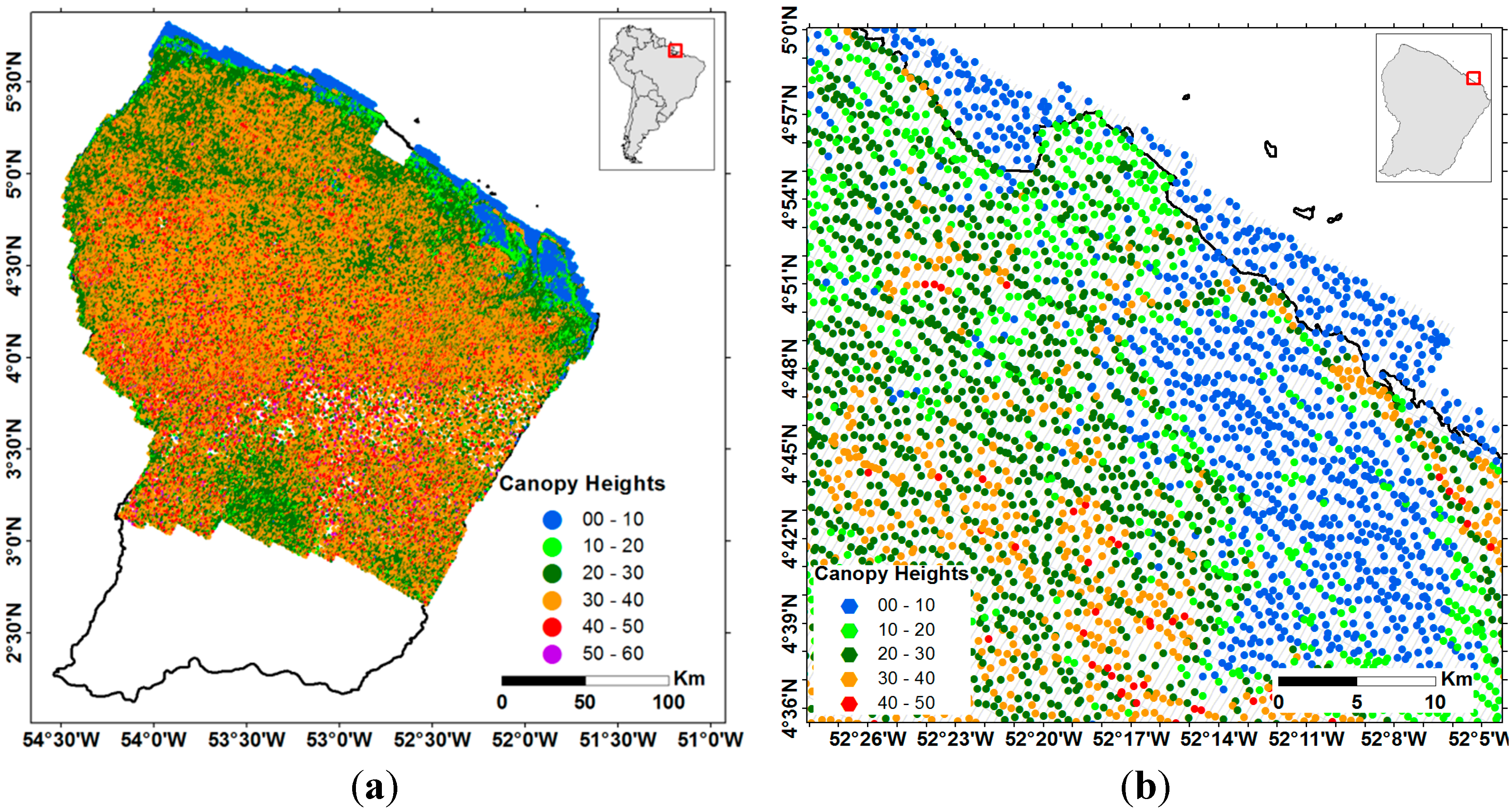
3.1.1. Processing the LD Dataset
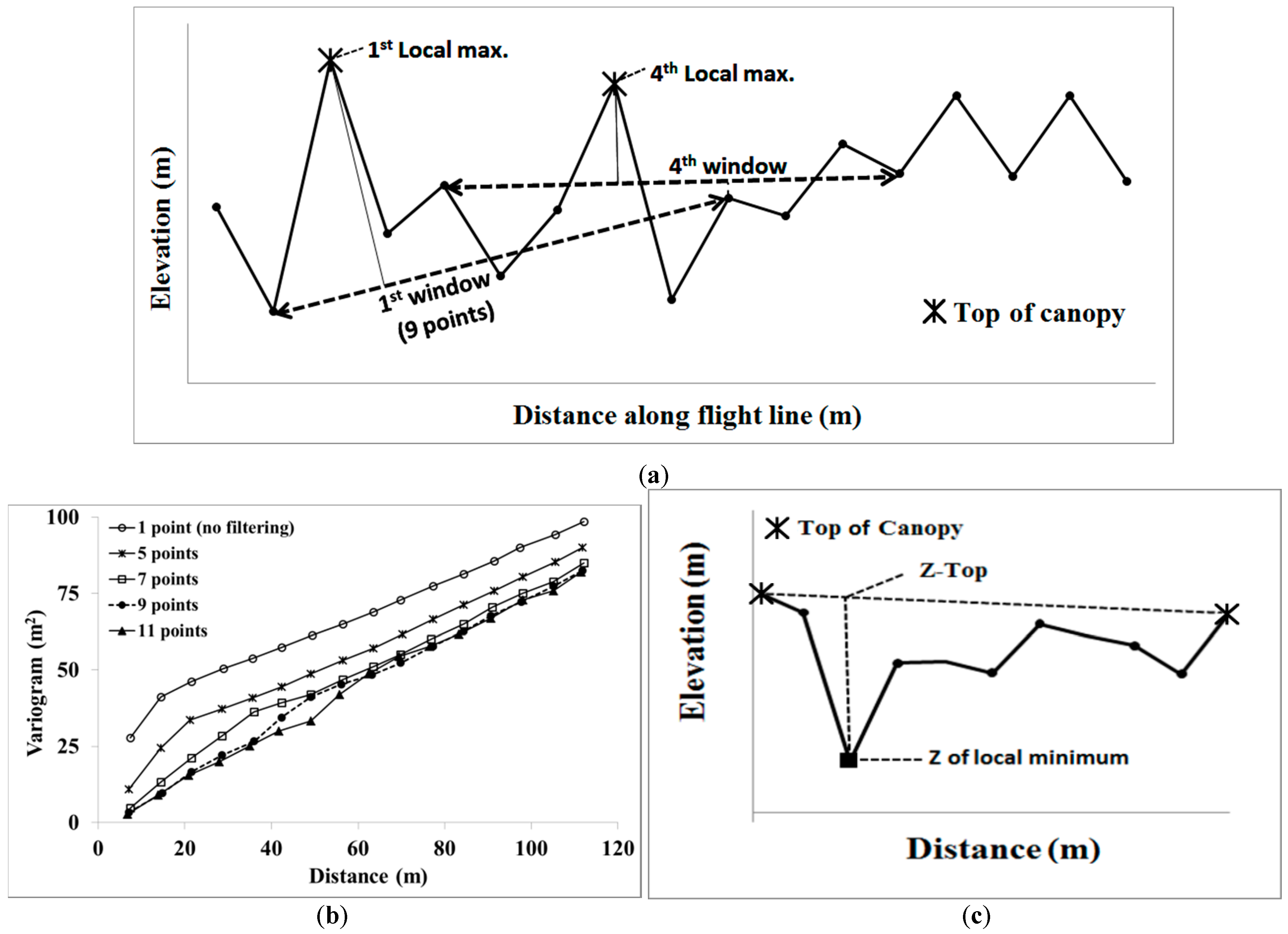
Data Filtering
Canopy Top Identification

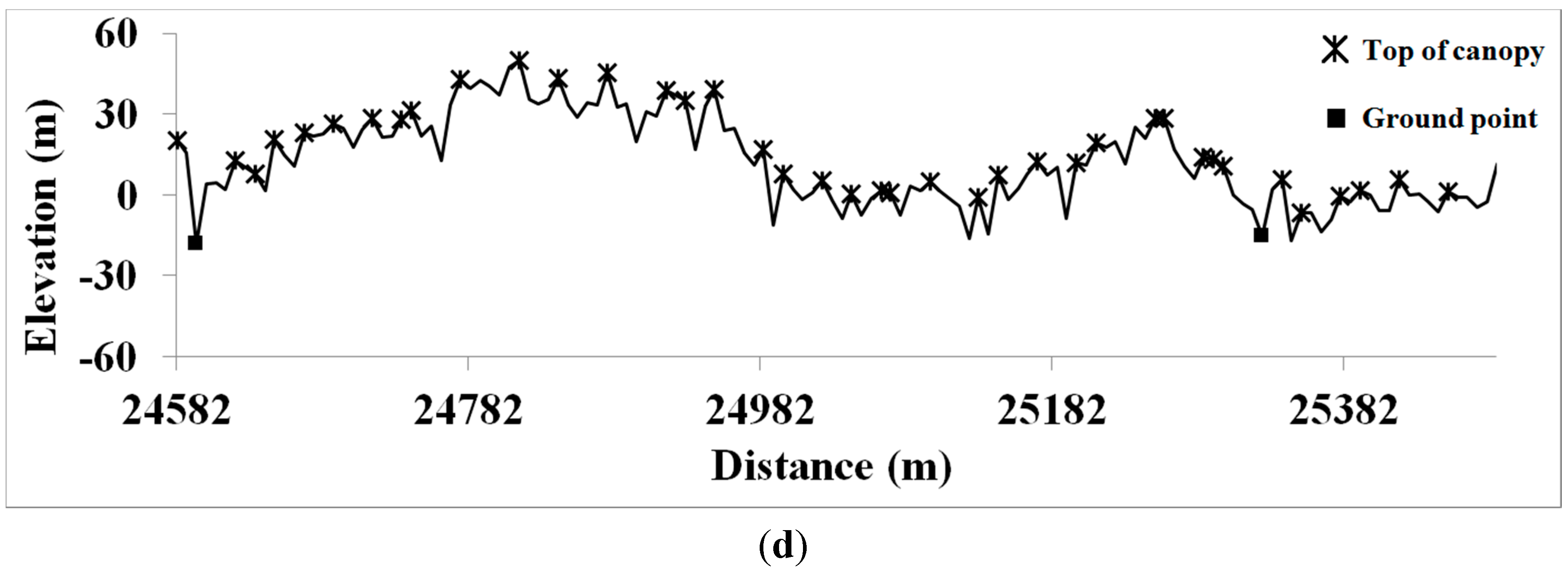
Identification of Ground Points
Canopy Height Estimation
3.1.2. Processing the HD Dataset
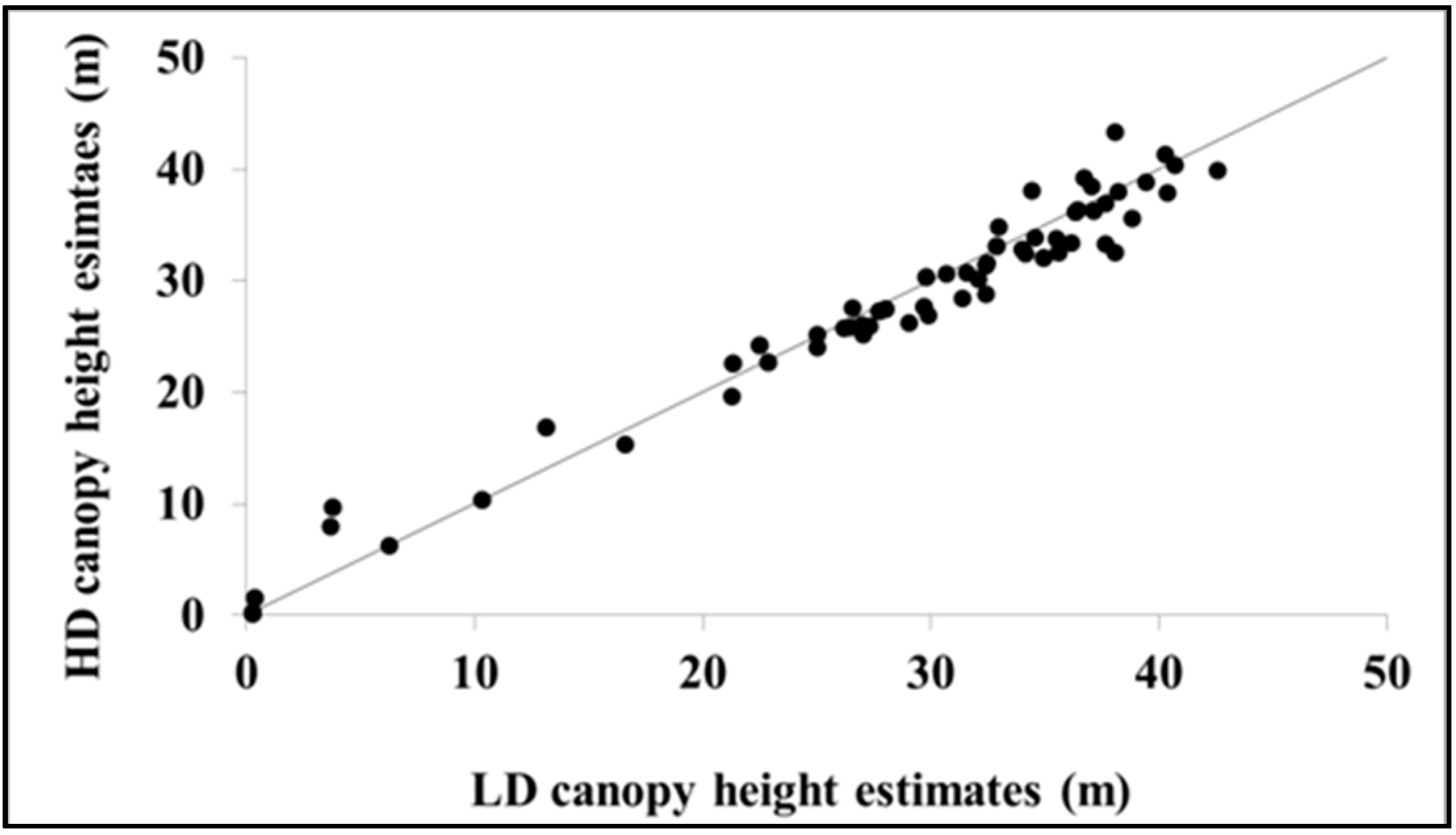
3.1.3. Comparison of Canopy Height Estimates from the LD and HD Datasets
3.2. GLAS Data Processing
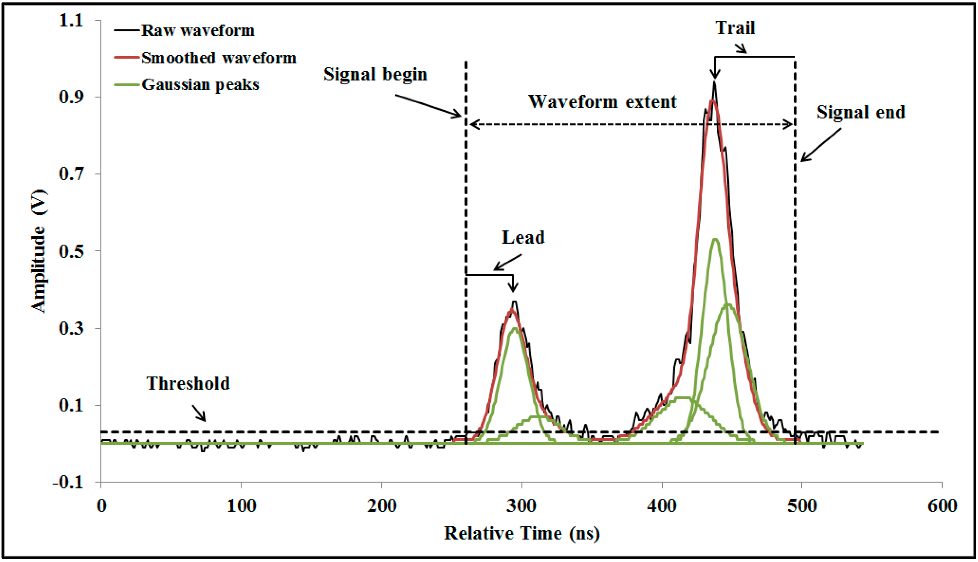
3.2.1. GLAS Waveform Metrics Extraction
3.2.2. Principal Component Analysis of GLAS Waveforms
3.3. Background on GLAS Canopy Height Estimation
3.3.1. Direct Method
3.3.2. Multiple Regression Models Using GLAS and DEM Metrics
| Model | ID | R2 | RMSE (m) | AIC |
|---|---|---|---|---|
| Hmax = Hb − Hg | 1 | 0.50 | 7.9 | 3126 |
| 2 | 0.72 | 4.9 | 2221 | |
| 2bis | 0.73 | 4.4 | 2185 | |
| 3 | 0.73 | 4.7 | 2223 | |
| 3bis | 0.73 | 4.6 | 2187 | |
| 4 | 0.80 | 3.9 | 2084 | |
| 4bis | 0.80 | 3.9 | 2081 | |
| 5 | 0.79 | 3.9 | 2096 | |
| 5bis | 0.79 | 3.9 | 2083 | |
| 6 | 0.85 | 4.0 | 2064 | |
| 6bis | 0.85 | 3.9 | 2056 | |
| 7 | 0.81 | 3.8 | 2063 | |
| 7bis | 0.81 | 3.7 | 2051 | |
| 8 | 0.81 | 3.8 | 2064 | |
| 8bis | 0.81 | 3.8 | 2056 | |
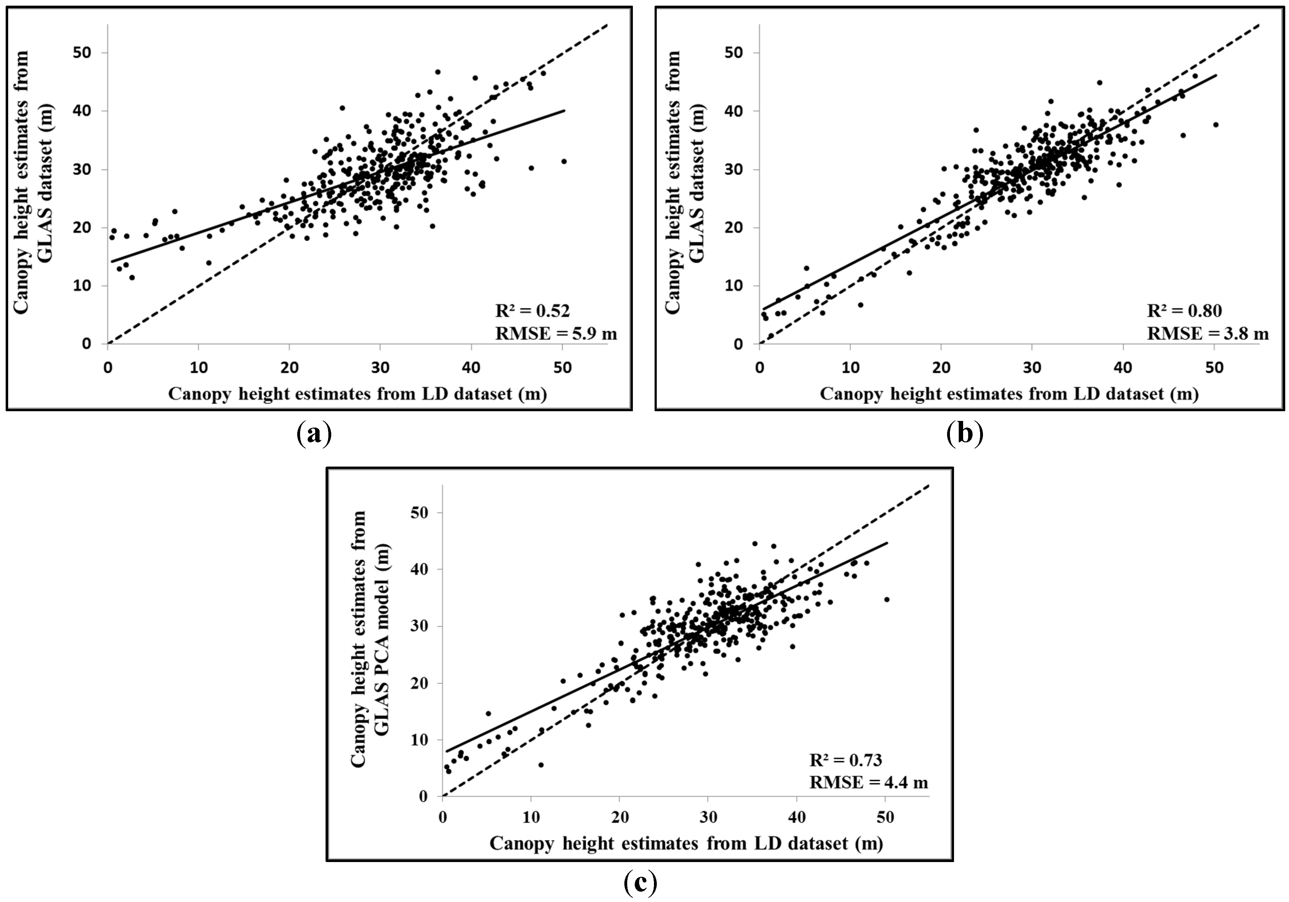
| 9 | 0.52 | 5.9 | 2373 | |
| Most important PCs (PC1, PC2, PC4, PC11) from ID 9 | 9bis | 0.47 | 6.2 | 2478 |
| 10 | 0.80 | 3.8 | 2047 | |
| Most important PCs (PC1, PC2, PC4, PC11) from ID 10 | 10bis | 0.79 | 3.9 | 2075 |
| 11 | 0.73 | 4.4 | 2174 | |
| 12 | 0.78 | 4.0 | 2064 | |
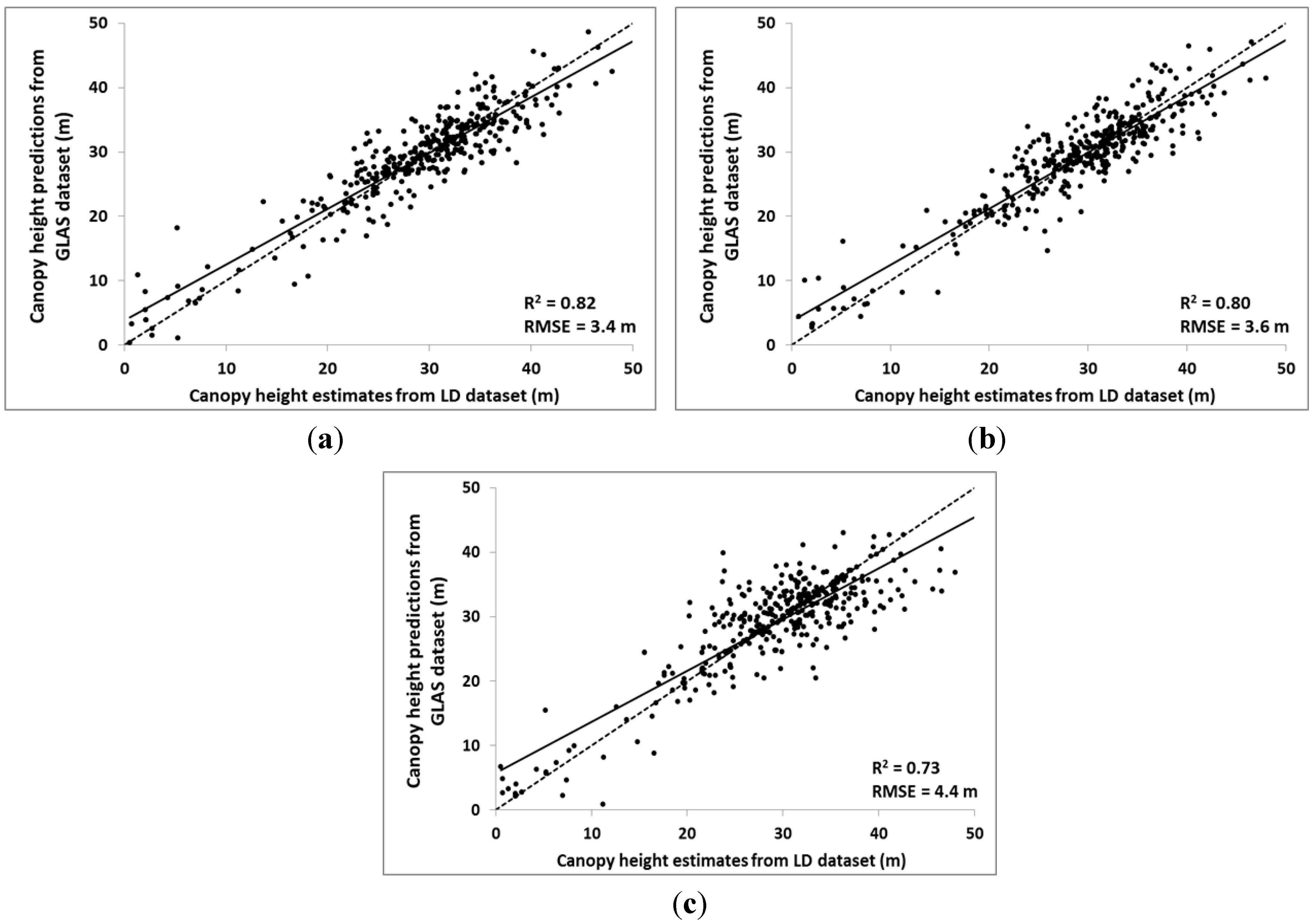
| Random Forest using: Wext + Lead + Trail + TI | 13 | 0.82 | 3.4 | - |
| Random Forest using: Wext + Lead + TI | 14 | 0.80 | 3.6 | - |
| Random Forest using: Wext + Lead | 15 | 0.80 | 3.6 | - |
| Random Forest using: Wext + TI | 16 | 0.82 | 3.6 | - |
| Random Forest using: Wext | 17 | 0.73 | 4.4 | - |
| Random Forest using: First 13 PC | 18 | 0.70 | 4.7 | - |
| Random Forest using: PC1 + PC2 + PC4 + PC11 | 18bis | 0.69 | 4.8 | - |
| Random Forest using: Wext and the first 13 PC | 19 | 0.83 | 3.6 | - |
| Random Forest using: Wext +PC1 + PC2 + PC4 + PC11 | 19bis | 0.82 | 3.6 | - |
| Random Forest using: WC and the first 13 PC | 20 | 0.81 | 3.7 | - |
| Random Forest using: WC +PC1 + PC2 + PC4 + PC11 | 20bis | 0.81 | 3.7 | - |
3.4. Proposed Techniques for Canopy Height Estimation
3.4.1. Multiple Regression Models Using Principal Components
3.4.2. Random Forest Regressions Using GLAS and DEM Metrics
3.4.3. Random Forest Regressions Using Principal Components
4. Results
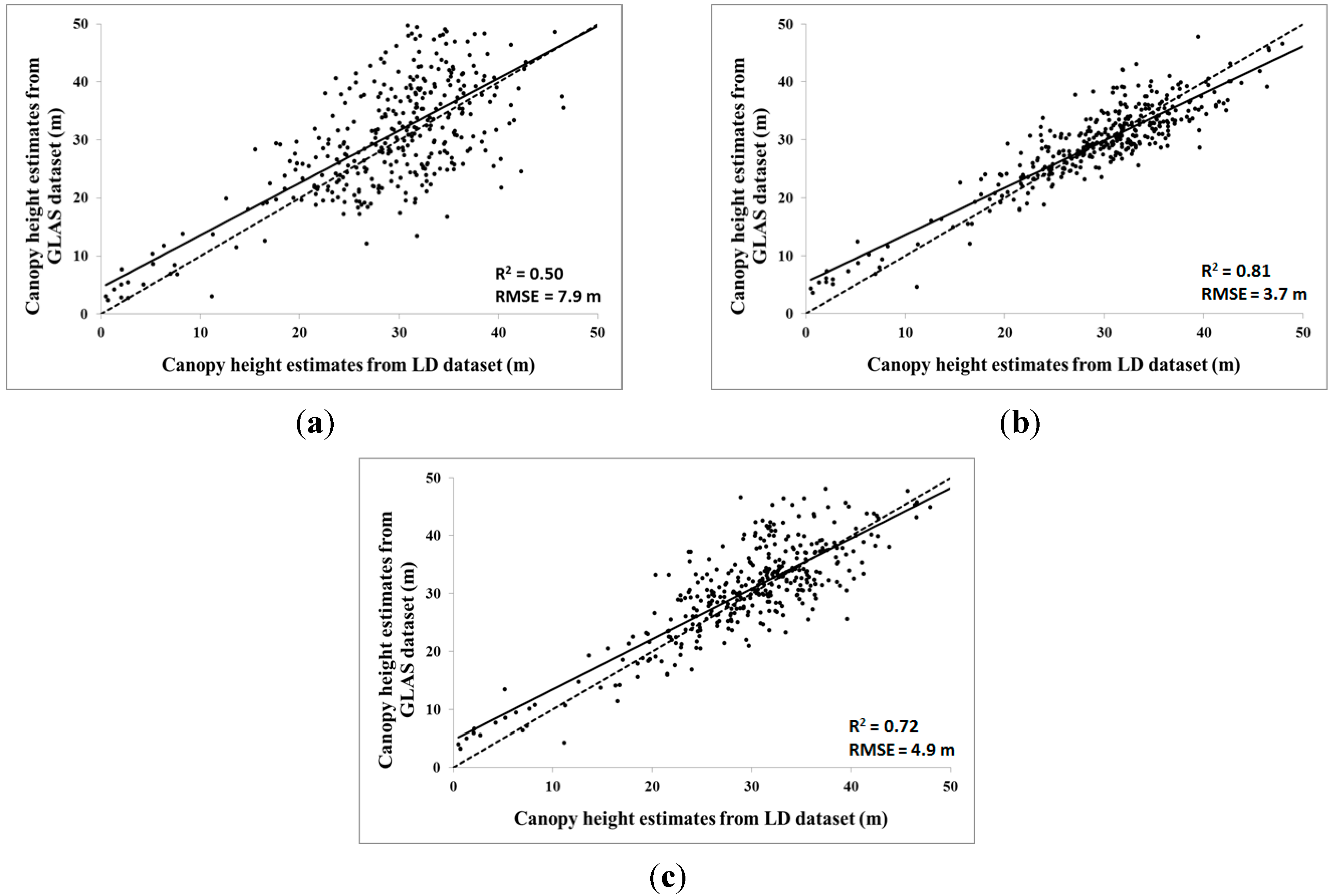
4.1. Direct Method
4.2. Multiple Regression Models
4.2.1. Using GLAS and DEM Metrics
4.2.2. Using Principal Components

4.3. Random Forest Regressions
4.3.1. Using GLAS and DEM Metrics

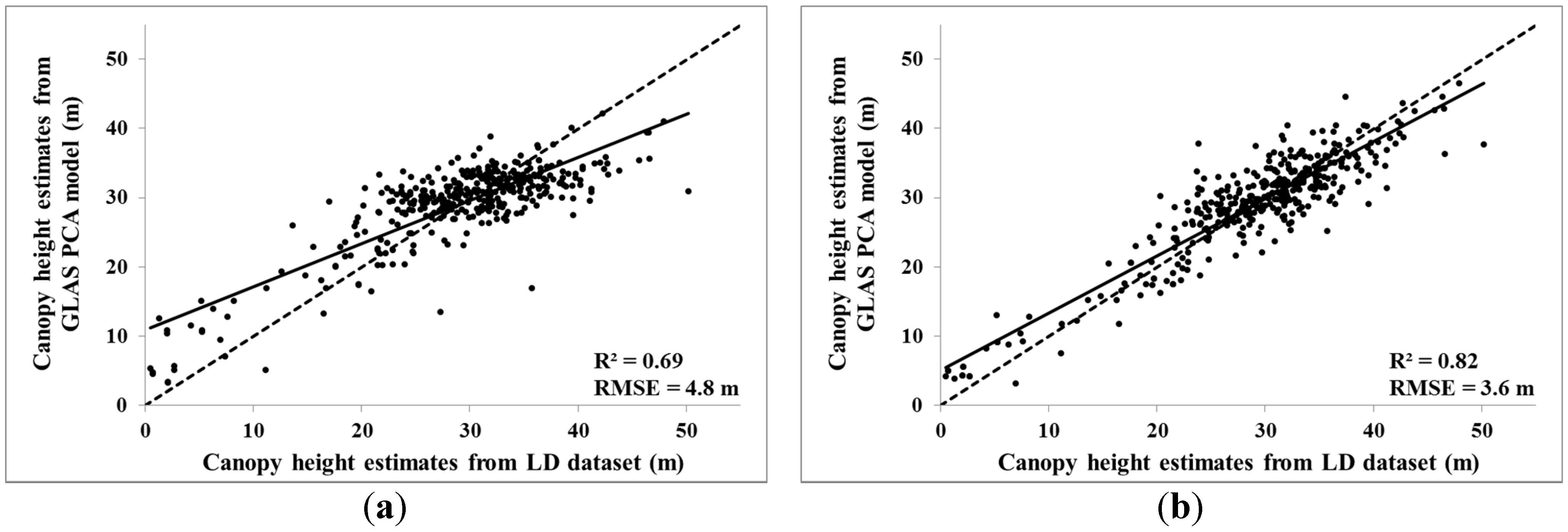
4.3.2. Using Principal Components
4.4. Model Performance in Different Forest Conditions
- -
- LT1 represents dense, closed-canopy forest with small crowns of the same canopy height and small gaps mixed with regular canopies with well-developed crowns of almost the same canopy height without large gaps interlaced with flooded savannas (10%).
- -
- LT2 is a closed canopy forest dominated by well-developed crowns of almost the same canopy height without large gaps.
- -
- LT3 is an irregular- and disrupted-canopy forest where the trees have very different heights and different crown diameters with large gaps mixed with closed-canopy forest dominated by well-developed crowns at almost the same elevation without large gaps. LT3 is also interlaced with liana forests.
- -
- LT4 is similar to LT3 with more liana forest and non-forest land covers.
- -
- LT5 is an open forest associated with wetlands and bamboo thickets. However, no GLAS footprints available over this LT.
4.5. Error on the Estimation of Biomass
5. Discussion
6. Conclusion
Acknowledgments
Author Contributions
Conflicts of Interest
References
- Pan, Y.; Birdsey, R.A.; Fang, J.; Houghton, R.; Kauppi, P.E.; Kurz, W.A.; Phillips, O.L.; Shvidenko, A.; Lewis, S.L.; Canadell, J.G.; et al. A large and persistent carbon sink in the world’s forests. Science 2011, 333, 988–993. [Google Scholar] [PubMed]
- Beer, C.; Reichstein, M.; Tomelleri, E.; Ciais, P.; Jung, M.; Carvalhais, N.; Rödenbeck, C.; Arain, M.A.; Baldocchi, D.; Bonan, G.B.; et al. Terrestrial gross carbon dioxide uptake: Global distribution and covariation with climate. Science 2010, 329, 834–838. [Google Scholar] [CrossRef] [PubMed]
- Chave, J.; Andalo, C.; Brown, S.; Cairns, M.A.; Chambers, J.Q.; Eamus, D.; Fölster, H.; Fromard, F.; Higuchi, N.; Kira, T.; et al. Tree allometry and improved estimation of carbon stocks and balance in tropical forests. Oecologia 2005, 145, 87–99. [Google Scholar] [CrossRef] [PubMed]
- Asner, G.P.; Mascaro, J. Mapping tropical forest carbon: Calibrating plot estimates to a simple LiDAR metric. Remote Sens. Environ. 2014, 140, 614–624. [Google Scholar] [CrossRef]
- Drake, J.B.; Knox, R.G.; Dubayah, R.O.; Clark, D.B.; Condit, R.; Blair, J.B.; Hofton, M. Above-ground biomass estimation in closed canopy neotropical forests using lidar remote sensing: Factors affecting the generality of relationships. Global Ecol. Biogeogr. 2003, 12, 147–159. [Google Scholar] [CrossRef]
- Feldpaush, T.R.; Lloyd, J.; Lewis, S.L.; Brienen, R.J.W.; Gloor, M.; Mendoza, A.M.; Lopez-Gonzalez, G.; Banin, L.; Salim, K.A.; Affum-Baffoe, K.; et al. Tree height integrated into pantropical forest biomass estimates. Biogeosciences 2012, 9, 3381–3403. [Google Scholar] [CrossRef] [Green Version]
- Lima, A.J.N.; Suwa, R.; de Mello Ribeiro, G.H.P.; Kajimoto, T.; dos Santos, J.; da Silva, R.P.; de Souza, C.A.S.; de Barros, P.C.; Noguchi, H.; Ishizuka, M.; et al. Allometric models for estimating above- and below-ground biomass in Amazonian forests at São Gabriel da Cachoeira in the upper Rio Negro, Brazil. Forest Ecol. Manag. 2012, 277, 163–172. [Google Scholar] [CrossRef]
- Maia Araújo, T.; Higuchi, N.; de Carvalho Júnior, J.A. Comparison of formulae for biomass content determination in a tropical rain forest site in the state of Pará, Brazil. Forest Ecol. Manag. 1999, 17, 43–52. [Google Scholar]
- Vieira, S.; de Camarago, P.B.; Selhorst, D.; da Silva, R.; Hutyra, L.; Chambers, J.Q.; Brown, I.F.; Higuchi, N.; dos Santos, J.; Wofsy, S.C.; et al. Forest structure and carbon dynamics in Amazonian tropical rain forests. Oecologia 2004, 140, 468–479. [Google Scholar] [CrossRef] [PubMed]
- Lefsky, M.A.; Harding, D.J.; Keller, M.; Cohen, W.B.; Carabajal, C.C.; Del Bom Espirito-Santo, F.; Hunter, M.O.; de Oliveira, R., Jr. Estimates of forest canopy height and aboveground biomass using ICESat. Geophys. Res. Lett. 2005, 32. [Google Scholar] [CrossRef]
- Mitchard, E.T.A.; Saatchi, S.S.; White, L.J.T.; Abernethy, K.A.; Jeffery, K.J.; Lewis, S.L.; Collins, M.; Lefsky, M.A.; Leal, M.E.; Woodhouse, I.H.; et al. Mapping tropical forest biomass with radar and spaceborne LiDAR in Lopé National Park, Gabon: Overcoming problems of high biomass and persistent cloud. Biogeosciences 2012, 9, 179–191. [Google Scholar] [CrossRef]
- Santoro, M.; Askne, J.; Dammert, P.B.G. Tree height estimation from multi-temporal ERS SAR interferometric phase omography. In Proceedings of FRINGE 2003 Workshop, Frascati, Italy, 1–5 December 2003.
- Praks, J.; Hallikainen, M.; Antropov, O.; Molina, D. Boreal forest tree height estimation from interferometric TanDEM-X images. In Proceedings of 2012 IEEE International Geoscience and Remote Sensing Symposium (IGARSS), Munich, Germany, 22–27 July 2012; pp. 1262–1265.
- Reigber, A.; Moreira, A. First demonstration of airborne SAR tomography using multibaseline L-band data. IEEE Trans. Geosci. Remote Sens. 2000, 38, 2142–2152. [Google Scholar] [CrossRef]
- Castel, T.; Beaudoin, A.; Trouche, G. Analysis of SAR interferometry for tree height estimation over hilly forested area. Agricultura 2002, 1, 15–23. [Google Scholar]
- Neumann, M.; Hensley, S.; Lavalle, M.; Ahmed, R. Forest Structure Characterization Using JPL’s UAVSAR Multi-Baseline polarimetric SAR interferometry and tomography. In Proceedings of The 4th Asia-Pacific Conference on Synthetic Aperture Radar, Tsukuba, Japan, 23–27 September 2013.
- Garestier, F.; Dubois-Fernandez, P.C.; Champion, I. Forest height inversion using high-resolution P-Band Pol-InSAR data. IEEE Trans. Geosci. Remote Sens. 2008, 46, 3544–3559. [Google Scholar] [CrossRef]
- Huang, Y.; Ferro-Famil, L.; Reigber, A. Under-foliage object imaging using SAR tomography and polarimetric spectral estimators. IEEE, Trans. Geosci. Remote Sens. 2011, 50, 2213–2225. [Google Scholar] [CrossRef]
- Guillaso, S.; Reigber, A. Scatterer characterisation using polarimetric SAR tomography. In Proceedings of 2005 IEEE International Geoscience and Remote Sensing Symposium, Seoul, Korea, 25–29 July 2005; pp. 2685–2688.
- Lefsky, M.A. A global forest canopy height map from the moderate resolution imaging spectroradiometer and the geoscience laser altimeter system. Geophys. Res. Lett. 2010, 37. [Google Scholar] [CrossRef]
- Wulder, M.A.; Seeman, D. Forest inventory height update through the integration of LIDAR data with segmented Landsat imagery. Can. J. Remote Sens. 2003, 29, 536–543. [Google Scholar] [CrossRef]
- Boudreau, J.; Nelson, R.F.; Margolis, H.A.; Beaudoin, A.; Guindon, L.; Kimes, D.S. Regional aboveground forest biomass using airborne and spaceborne LiDAR in Québec. Remote Sens. Environ. 2008, 112, 3876–3890. [Google Scholar] [CrossRef]
- Saatchi, S.S.; Harris, N.L.; Brown, S.; Lefsky, M.; Mitchard, E.T.A.; Salas, W.; Zutta, B.R.; Buermann, W.; Lewis, S.L.; Hagen, S.; et al. Benchmark map of forest carbon stocks in tropical regions across three continents. Proc. Natl. Acad. Sci. 2011, 108, 9899–9904. [Google Scholar] [CrossRef] [PubMed]
- Hilbert, C.; Schmullius, C. Influence of surface topography on ICESat/GLAS forest height estimation and waveform shape. Remote Sens. 2012, 4, 2210–2235. [Google Scholar] [CrossRef]
- Lee, S.; Ni-Meister, W.; Yang, W.; Chen, Q. Physically based vertical vegetation structure retrieval from ICESat data: Validation using LVIS in White Mountain National Forest, New Hampshire, USA. Remote Sens. Environ. 2011, 115, 2776–2785. [Google Scholar] [CrossRef]
- Pang, Y.; Lefsky, M.; Andersen, H.-E.; Miller, M.E.; Sherrill, K. Validation of the ICEsat vegetation product using crown-area-weighted mean height derived using crown delineation with discrete return lidar data. Can. J. Remote Sens. 2008, 34, S471–S484. [Google Scholar] [CrossRef]
- Ploton, P.; Pélissier, R.; Barbier, N.; Proisy, C.; Ramesh, B.R.; Couteron, P. Canopy texture analysis for large-scale assessments of tropical forest stand structure and biomass. In Treetops at Risk; Lowman, M., Devy, S., Ganesh, T., Eds.; Springer New York: New York, NY, USA, 2013; pp. 237–245. [Google Scholar]
- Lu, D.; Chen, Q.; Wang, G.; Moran, E.; Batistella, M.; Zhang, M.; Laurin, G.V.; Saah, D. Aboveground forest biomass estimation with Landsat and lidar data and uncertainty analysis of the estimates. Int. J. For. Res. 2012, 2012, 1–16. [Google Scholar]
- Proisy, C.; Mougin, E.; Fromard, F.; Karam, M.A. Interpretation of polarimetric radar signatures of mangrove forests. Remote Sens. Environ. 2000, 71, 56–66. [Google Scholar] [CrossRef]
- Le Toan, T.; Quegan, S.; Davidson, M.W.J.; Balzter, H.; Paillou, P.; Papathanassiou, K.; Plummer, S.; Rocca, F.; Saatchi, S.; Shugart, H.; et al. The BIOMASS mission: Mapping global forest biomass to better understand the terrestrial carbon cycle. Remote Sens. Environ. 2011, 115, 2850–2860. [Google Scholar] [CrossRef]
- Sandberg, G.; Ulander, L.M.H.; Fransson, J.E.S.; Holmgren, J.; Le Toan, T. L- and P-band backscatter intensity for biomass retrieval in hemiboreal forest. Remote Sens. Environ. 2011, 115, 2874–2886. [Google Scholar] [CrossRef]
- Wu, S.-T. Potential application of multipolarization SAR for pine-plantation biomass estimation. IEEE Trans. Geosci. Remote Sens. 1987, GE-25, 403–409. [Google Scholar] [CrossRef]
- Dobson, M.C.; Ulaby, F.T.; LeToan, T.; Beaudoin, A.; Kasischke, E.S.; Christensen, N. Dependence of radar backscatter on coniferous forest biomass. IEEE Trans. Geosci. Remote Sens. 1992, 30, 412–415. [Google Scholar] [CrossRef]
- Imhoff, M.L. Radar backscatter and biomass saturation: Ramifications for global biomass inventory. IEEE Trans. Geosci. Remote Sens. 1995, 33, 511–518. [Google Scholar] [CrossRef]
- Luckman, A.; Baker, J.; Kuplich, T.M.; da Costa Freitas Yanasse, C.; Frery, A.C. A study of the relationship between radar backscatter and regenerating tropical forest biomass for spaceborne SAR instruments. Remote Sens. Environ. 1997, 60, 1–13. [Google Scholar] [CrossRef]
- Luckman, A.; Baker, J.; Honzák, M.; Lucas, R. Tropical forest biomass density estimation using JERS-1 SAR: Seasonal variation, confidence limits, and application to image mosaics. Remote Sens. Environ. 1998, 63, 126–139. [Google Scholar] [CrossRef]
- Minh, D.H.T.; Le Toan, T.; Rocca, F.; Tebaldini, S.; d’Alessandro, M.M.; Villard, L. Relating P-band synthetic aperture radar tomography to tropical forest biomass. IEEE Trans. Geosci. Remote Sens. 2014, 52, 967–979. [Google Scholar] [CrossRef]
- Nizalapur, V.; Sekhar Jha, C.; Madugundu, R. Estimation of above ground biomass in Indian tropical forested area using multifrequency DLRESAR data. Int. J. Geomat. Geosci. 2010, 1, 167–178. [Google Scholar]
- Zolkos, S.G.; Goetz, S.J.; Dubayah, R. A meta-analysis of terrestrial aboveground biomass estimation using lidar remote sensing. Remote Sens. Environ. 2013, 128, 289–298. [Google Scholar] [CrossRef]
- Chen, Q. Retrieving vegetation height of forests and woodlands over mountainous areas in the Pacific Coast region using satellite laser altimetry. Remote Sens. Environ. 2010, 114, 1610–1627. [Google Scholar] [CrossRef]
- Bourgine, B.; Baghdadi, N. Assessment of C-band SRTM DEM in a dense equatorial forest zone. Compt. Rendus Geosci. 2005, 337, 1225–1234. [Google Scholar] [CrossRef]
- Bourgine, B.; Baghdadi, N.; Hosford, S.; Daniels, P. Generation of a ground-level DEM in a dense equatorial forest zone by merging airborne laser data and a top-of-canopy DEM. Can. J. Remote Sens. 2004, 30, 913–926. [Google Scholar] [CrossRef]
- Vincent, G.; Caron, F.; Sabatier, D.; Blanc, L. LiDAR shows that higher forests have more slender trees. Bois. Forêts Tropiques 2012, 314, 51–56. [Google Scholar]
- Harding, D.J.; Carabajal, C.C. ICESat waveform measurements of within-footprint topographic relief and vegetation vertical structure. Geophys. Res. Lett. 2005, 32. [Google Scholar] [CrossRef]
- Baghdadi, N.; Le Maire, G.; Fayad, I.; Bailly, J.S.; Nouvellon, Y.; Lemos, C.; Hakamada, R. Testing different methods of forest height and aboveground biomass estimations from ICESat/GLAS data in Eucalyptus plantations in Brazil. IEEE J. Sel. Top. Appl. Earth Obs. Remote Sens. 2014, 7, 290–299. [Google Scholar] [CrossRef]
- Baghdadi, N.; Cavelier, S.; Chiles, J.-P.; Bourgine, B.; Toutin, T.; King, C.; Daniels, P.; Perrin, J.; Truffert, C. Merging of airborne elevation data and Radarsat data to develop a Digital Elevation Model. Int. J. Remote Sens. 2005, 26, 139–163. [Google Scholar] [CrossRef]
- Rosette, J.A.B.; North, P.R.J.; Suarez, J.C. Vegetation height estimates for a mixed temperate forest using satellite laser altimetry. Int. J. Remote Sens. 2008, 29, 1475–1493. [Google Scholar] [CrossRef]
- Lefsky, M.A.; Keller, M.; Pang, Y.; De Camargo, P.B.; Hunter, M.O. Revised method for forest canopy height estimation from Geoscience Laser Altimeter System waveforms. J. Appl. Remote Sens. 2007, 1. [Google Scholar] [CrossRef]
- Sun, G.; Ranson, K.J.; Kimes, D.S.; Blair, J.B.; Kovacs, K. Forest vertical structure from GLAS: An evaluation using LVIS and SRTM data. Remote Sens. Environ. 2008, 112, 107–117. [Google Scholar] [CrossRef]
- Duong, H.; Lindenbergh, R.; Pfeifer, N.; Vosselman, G. ICESat full-waveform altimetry compared to airborne LASER scanning altimetry over The Netherlands. IEEE Trans. Geosci. Remote Sens. 2009, 47, 3365–3378. [Google Scholar] [CrossRef]
- Allouis, T.; Bailly, J.-S.; Pastol, Y.; Le Roux, C. Comparison of LiDAR waveform processing methods for very shallow water bathymetry using Raman, near-infrared and green signals. Earth Surf. Process. Landf. 2010, 35, 640–650. [Google Scholar]
- Karlis, D.; Saporta, G.; Spinakis, A. A simple rule for the selection of principal components. Commun. Stat.—Theory Methods 2003, 32, 643–666. [Google Scholar] [CrossRef]
- Neuenschwander, A.L.; Magruder, L.A.; Tyler, M. Landcover classification of small-footprint, full-waveform lidar data. J. Appl. Remote Sens. 2009, 3. [Google Scholar] [CrossRef]
- Carabajal, C.C.; Harding, D.J. SRTM C-band and ICESat laser altimetry elevation comparisons as a function of tree cover and relief. Photogramm. Eng. Remote Sens. 2006, 72, 287–298. [Google Scholar] [CrossRef]
- Duncanson, L.I.; Niemann, K.O.; Wulder, M.A. Estimating forest canopy height and terrain relief from GLAS waveform metrics. Remote Sens. Environ. 2010, 114, 138–154. [Google Scholar] [CrossRef]
- Akaike, H. Information theory and an extension of the maximum likelihood principle. In Selected Papers of Hirotugu Akaike; Parzen, E., Tanabe, K., Kitagawa, G., Eds.; Springer New York: New York, NY, USA, 1998; pp. 199–213. [Google Scholar]
- Houghton, R.A.; Butman, D.; Bunn, A.G.; Krankina, O.N.; Schlesinger, P.; Stone, T.A. Mapping Russian forest biomass with data from satellites and forest inventories. Environ. Res. Lett. 2007, 2. [Google Scholar] [CrossRef]
- Kankare, V.; Vastaranta, M.; Holopainen, M.; Räty, M.; Yu, X.; Hyyppä, J.; Hyyppä, H.; Alho, P.; Viitala, R. Retrieval of forest aboveground biomass and stem volume with airborne scanning LiDAR. Remote Sens. 2013, 5, 2257–2274. [Google Scholar] [CrossRef] [Green Version]
- Le Maire, G.; Marsden, C.; Nouvellon, Y.; Grinand, C.; Hakamada, R.; Stape, J.-L.; Laclau, J.-P. MODIS NDVI time-series allow the monitoring of Eucalyptus plantation biomass. Remote Sens. Environ. 2011, 115, 2613–2625. [Google Scholar] [CrossRef]
- Mutanga, O.; Adam, E.; Cho, M.A. High density biomass estimation for wetland vegetation using WorldView-2 imagery and random forest regression algorithm. Int. J. Appl. Earth Obs. Geoinf. 2012, 18, 399–406. [Google Scholar] [CrossRef]
- Breiman, L. Random forests. Mach. Learn. 2001, 45, 5–32. [Google Scholar] [CrossRef]
- Gond, V.; Freycon, V.; Molino, J.-F.; Brunaux, O.; Ingrassia, F.; Joubert, P.; Pekel, J.-F.; Prévost, M.-F.; Thierron, V.; Trombe, P.-J.; et al. Broad-scale spatial pattern of forest landscape types in the Guiana Shield. Int. J. Appl. Earth Obs. Geoinf. 2011, 13, 357–367. [Google Scholar] [CrossRef]
- Asner, G.P.; Mascaro, J.; Muller-Landau, H.C.; Vieilledent, G.; Vaudry, R.; Rasamoelina, M.; Hall, J.S.; van Breugel, M. A universal airborne LiDAR approach for tropical forest carbon mapping. Oecologia 2012, 168, 1147–1160. [Google Scholar] [CrossRef] [PubMed]
- Houghton, R.A.; Hall, F.; Goetz, S.J. Importance of biomass in the global carbon cycle. J. Geophys. Res. 2009, 114. [Google Scholar] [CrossRef]
- Hall, F.G.; Bergen, K.; Blair, J.B.; Dubayah, R.; Houghton, R.; Hurtt, G.; Kellndorfer, J.; Lefsky, M.; Ranson, J.; Saatchi, S.; et al. Characterizing 3D vegetation structure from space: Mission requirements. Remote Sens. Environ. 2011, 115, 2753–2775. [Google Scholar] [CrossRef]
© 2014 by the authors; licensee MDPI, Basel, Switzerland. This article is an open access article distributed under the terms and conditions of the Creative Commons Attribution license (http://creativecommons.org/licenses/by/4.0/).
Share and Cite
Fayad, I.; Baghdadi, N.; Bailly, J.-S.; Barbier, N.; Gond, V.; Hajj, M.E.; Fabre, F.; Bourgine, B. Canopy Height Estimation in French Guiana with LiDAR ICESat/GLAS Data Using Principal Component Analysis and Random Forest Regressions. Remote Sens. 2014, 6, 11883-11914. https://doi.org/10.3390/rs61211883
Fayad I, Baghdadi N, Bailly J-S, Barbier N, Gond V, Hajj ME, Fabre F, Bourgine B. Canopy Height Estimation in French Guiana with LiDAR ICESat/GLAS Data Using Principal Component Analysis and Random Forest Regressions. Remote Sensing. 2014; 6(12):11883-11914. https://doi.org/10.3390/rs61211883
Chicago/Turabian StyleFayad, Ibrahim, Nicolas Baghdadi, Jean-Stéphane Bailly, Nicolas Barbier, Valéry Gond, Mahmoud El Hajj, Frédéric Fabre, and Bernard Bourgine. 2014. "Canopy Height Estimation in French Guiana with LiDAR ICESat/GLAS Data Using Principal Component Analysis and Random Forest Regressions" Remote Sensing 6, no. 12: 11883-11914. https://doi.org/10.3390/rs61211883