Classifier Directed Data Hybridization for Geographic Sample Supervised Segment Generation

Abstract

Quality segment generation is a well-known challenge and research objective within Geographic Object-based Image Analysis (GEOBIA). Although methodological avenues within GEOBIA are diverse, segmentation commonly plays a central role in most approaches, influencing and being influenced by surrounding processes. A general approach using supervised quality measures, specifically user provided reference segments, suggest casting the parameters of a given segmentation algorithm as a multidimensional search problem. In such a sample supervised segment generation approach, spatial metrics observing the user provided reference segments may drive the search process. The search is commonly performed by metaheuristics. A novel sample supervised segment generation approach is presented in this work, where the spectral content of provided reference segments is queried. A one-class classification process using spectral information from inside the provided reference segments is used to generate a probability image, which in turn is employed to direct a hybridization of the original input imagery. Segmentation is performed on such a hybrid image. These processes are adjustable, interdependent and form a part of the search problem. Results are presented detailing the performances of four method variants compared to the generic sample supervised segment generation approach, under various conditions in terms of resultant segment quality, required computing time and search process characteristics. Multiple metrics, metaheuristics and segmentation algorithms are tested with this approach. Using the spectral data contained within user provided reference segments to tailor the output generally improves the results in the investigated problem contexts, but at the expense of additional required computing time.

1. Introduction

Remotely sensed satellite imagery has unique characteristics and derived information products compared to imagery encountered in many other image analysis disciplines. Various sub-elements in such imagery may need to be recognized and their attributes quantified. Land-cover mapping is a common task in this context, where it is attempted to generate a partial or full description of a given area from Earth observation imagery, with an emphasis on element geometric and thematic accuracies. Geographic Object-Based Image Analysis (GEOBIA) has emerged as a viable avenue of approaches, or paradigm, to tackle such remote sensing image analysis tasks [1,2,3,4] due to the common spectral-textural-geometric and thematic correlations of elements of interest in satellite imagery [5,6,7].

Incorporating a segmentation algorithm, which is central in many GEOBIA approaches, either for semantic object segmentation and description [8], or for only allowing for the generation of richer attributes for classification, have been shown to be efficient in many real world applications [2]. This is partly due to the h-res phenomenon [9] encountered commonly when concerned with Very High Resolution (VHR) optical imagery, where the spatial resolution of captured imagery is finer than the geometry of the elements of interest and pixel-based discriminative methods are limited to produce adequate results (due to the so called salt-and-pepper effect [10]). Also, such fidelity in resolution may be needed to identify elements, but intra element spectral variability may additionally cause problems in this process [11]. Segmentation algorithms allowing for spatial aggregation in addition to observing spectral characteristics have been shown to be efficient in working towards identifying elements [7,11,12,13,14]. Based on the characteristics of the desired information products and the nature of the data, the availability of commercial and freeware GEOBIA software [2,15,16,17] and the extent of the literature [1,2,4], it is shown that GEOBIA is a promising paradigm [1].

Although thematically accurate segments are commonly aimed for in a GEOBIA workflow, adequate segmentation is problematic to attain for single or multiclass elements using only a single pass of a given segmentation algorithm. This may be due to the complexity of the scene, especially when thematic and spectral correlations start to diverge, and limitations of the given segmentation algorithm. Various general approaches have been proposed to address the challenge of thematically accurate image segmentation and classification (semantic segmentation), including advocating rule-set or expert system’s approaches within GEOBIA [1,14], the development of new domain specific segmentation algorithms [18], multi-scale image analysis [6,19,20], using context information or spatial relationships among segments [14,21,22], and hybridizing or interleaving classification and segmentation processes [23,24,25]. Another general approach addressing the problem of segmentation within GEOBIA casts the creation of thematically accurate image segments as a search or optimization problem [26,27,28,29]. In such an approach the parameters of a given segmentation algorithm is automatically tuned based on the provision of a limited amount of user provided reference segments. The geometric aspects of provided reference segments are matched with generated segments in the iterative search process via spatial metrics.

In this work a novel variant of such a sample supervised segment generation approach is presented and quantitatively evaluated. The initial concept was presented in abstract from in [30]. An enlarged search space is defined to include pixel-based classification processes. Derived probability images are used to direct a change in the original input imagery, such that the given segmentation algorithm may perform better on the given problem. The proposed method is compared with the generic formulation of sample supervised segment generation and results are demonstrated via the task of accurately segmenting structures in towns, villages and refugee camps on VHR optical remote sensing data. This contribution thus falls within the context of enlarged search spaces first presented in [29], but proposes a methodology that uses spectral content contained within reference segments as opposed to adding data transformation or mapping functions.

Section 2 gives an overview of sample supervised segment generation and reviews related work. In Section 3 a new variant of sample supervised segment generation is presented, incorporating classification in the segment generation process. In Section 4 the data used is briefly described, with the comparative experimental methodologies outlined in Section 5. In Section 6 results are presented and discussed. Prospects and limitations are highlighted in Section 7.

2. Background and Related Work

Sample supervised segment generation, or more generally sample supervised image processing/analysis, denotes the process of automatically tuning the parameters of a given segmentation algorithm or constructing image processing operators for segment generation based on the provision of exemplar output segments. A user typically needs to digitize or provide examples of desired segmentation results. Such an approach has attracted research attention in the imaging disciplines in general [26,28,31,32,33,34,35] and also more specifically in the context of remote sensing image analysis [27,29,36]. It is a feasible strategy if a scene contains numerous “similar” elements that are of interest, common in many mapping tasks. Unsupervised strategies, not requiring reference segments but using scene wide image statistics, are also pursued [19]. It should be noted that the uses of efficient search methods are diverse in the imaging disciplines, with attribute selection and feature creation other common applications [37,38].

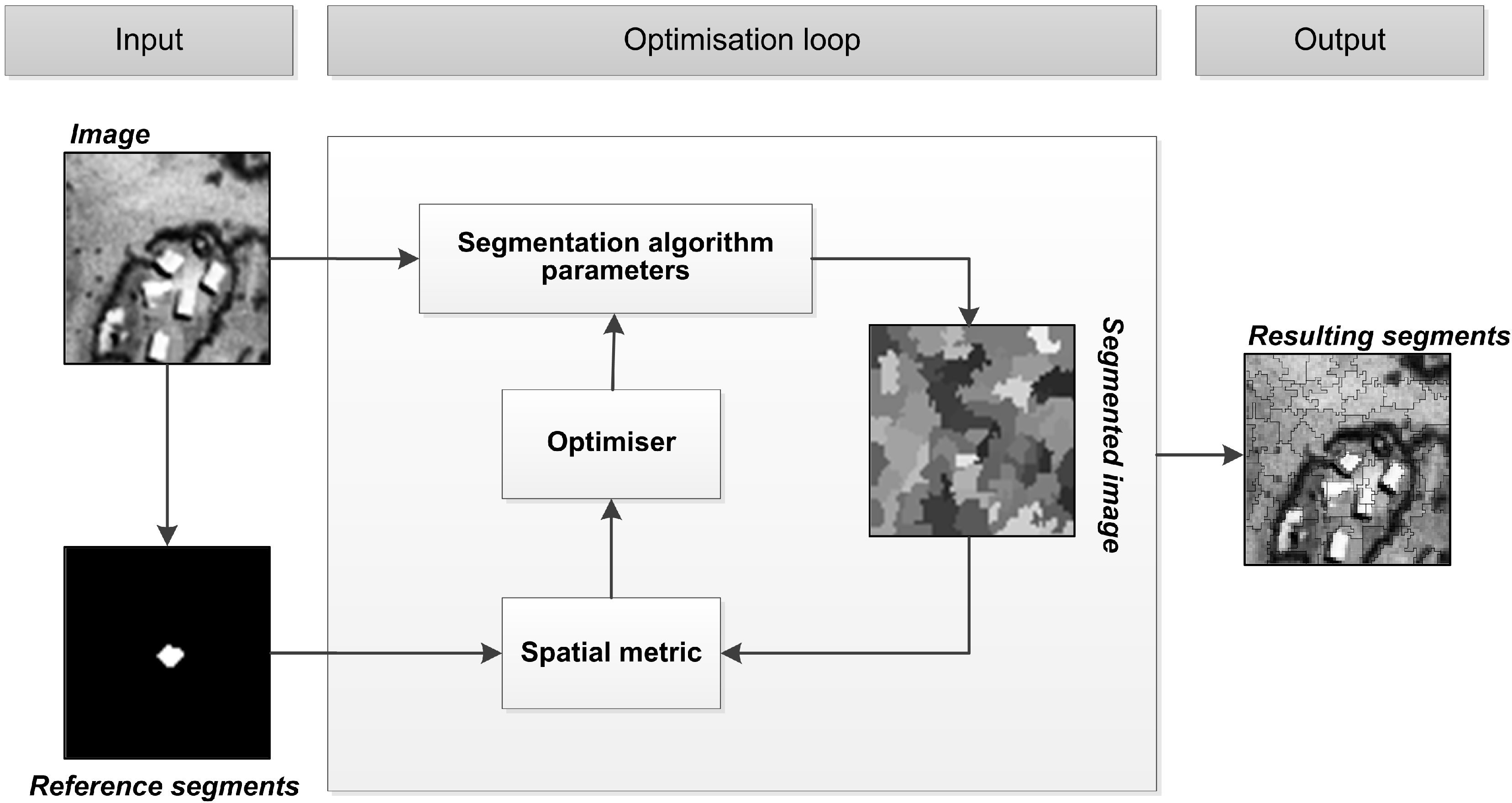
Figure 1 [39] illustrates the generic formulation of such an approach. A user provides a selection of reference segments or objects, typically digitized or extracted with other tools [40]. An iterative search process is invoked, where the parameter space of a given segmentation algorithm is searched. At iterations of the search process a specific parameter set is passed onto the segmentation algorithm from the optimizer. The tuned segmentation algorithm is executed on the image, typically subsets of the image covering areas around the provided reference segments. Empirical discrepancy, or spatial metrics [41] are employed to match the generated segments to that of the user provided reference segments. This process is commonly referred to as the fitness evaluation. The optimizer uses the quality score generated by the metrics to direct the next iteration of the search. The method terminates when a certain number of search iterations have passed or a certain quality threshold has been reached, although various other stopping criteria may be considered. The parameter set resulting in the best metric score is given as the output. Subsequently, the entire scene may be segmented with the segmentation algorithm tuned with the output parameter set.

Figure 1. Architecture of the generic formulation of sample supervised segment generation [39].

Figure 1. Architecture of the generic formulation of sample supervised segment generation [39].

A sample supervised segment generation method typically advocates an interactive, user driven image analysis process. Segmentation is, generally computationally expensive, resulting in computationally expensive fitness evaluations. Searching the parameter space efficiently was a major driver for the development of this method [26]. Metaheuristics, which are stochastic population based search methods, are well suited and studied in the context of this general approach [26,29,42,43], commonly leading to higher quality fitness scores in less search time compared to more general search strategies. Such a general approach may also be used to compare segmentation algorithms for a given task, or purely to test the general feasibility of a given algorithm for a given task. Also, this approach may find use alongside other, more encompassing, image analysis strategies. It could be used to work towards a final product in complex scene scenarios or used alongside traditional GEOBIA approaches such as rule set development [14].

Research on this general method typically aims for generating better quality results in less time. Specific aspects investigated include the evaluation of the performances of different search methods [29,42,43,44], the applicability of various empirical discrepancy metrics (fitness functions) [29,36], the performances of various segmentation algorithms in such an approach [29,42,45,46,47] and the extension of the concept to more modular image processing methods [24,45,46,47,48,49,50]. Uncertainties remain surrounding the generalizability of such a method, its sampling size requirements and whether strong correlations exist between classification results and segmentation [27,29]. Research and freeware software in this vein are available [29,42,51]. Having some a priori knowledge on the capability of the segmentation algorithm seems necessary [27].

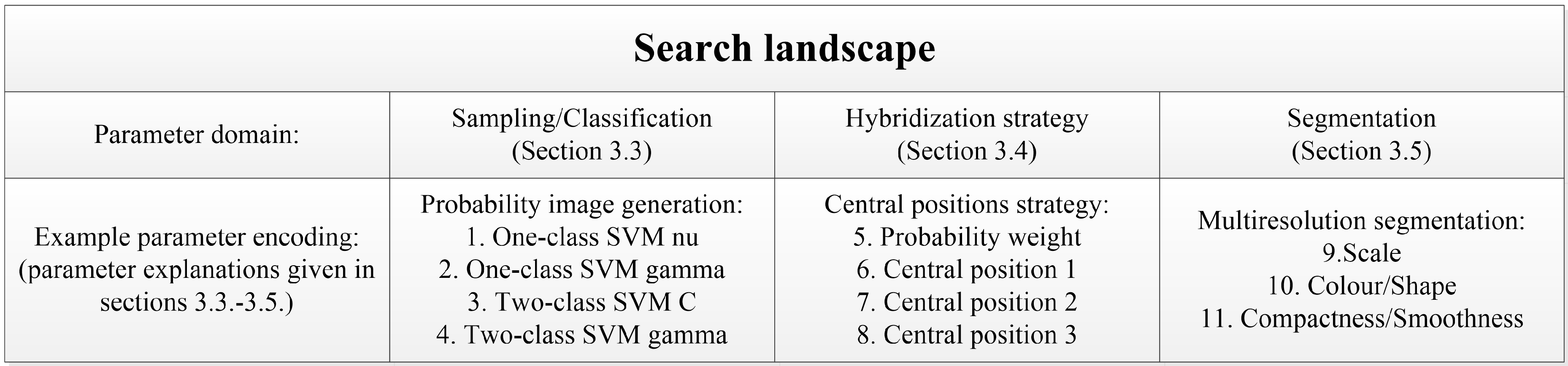
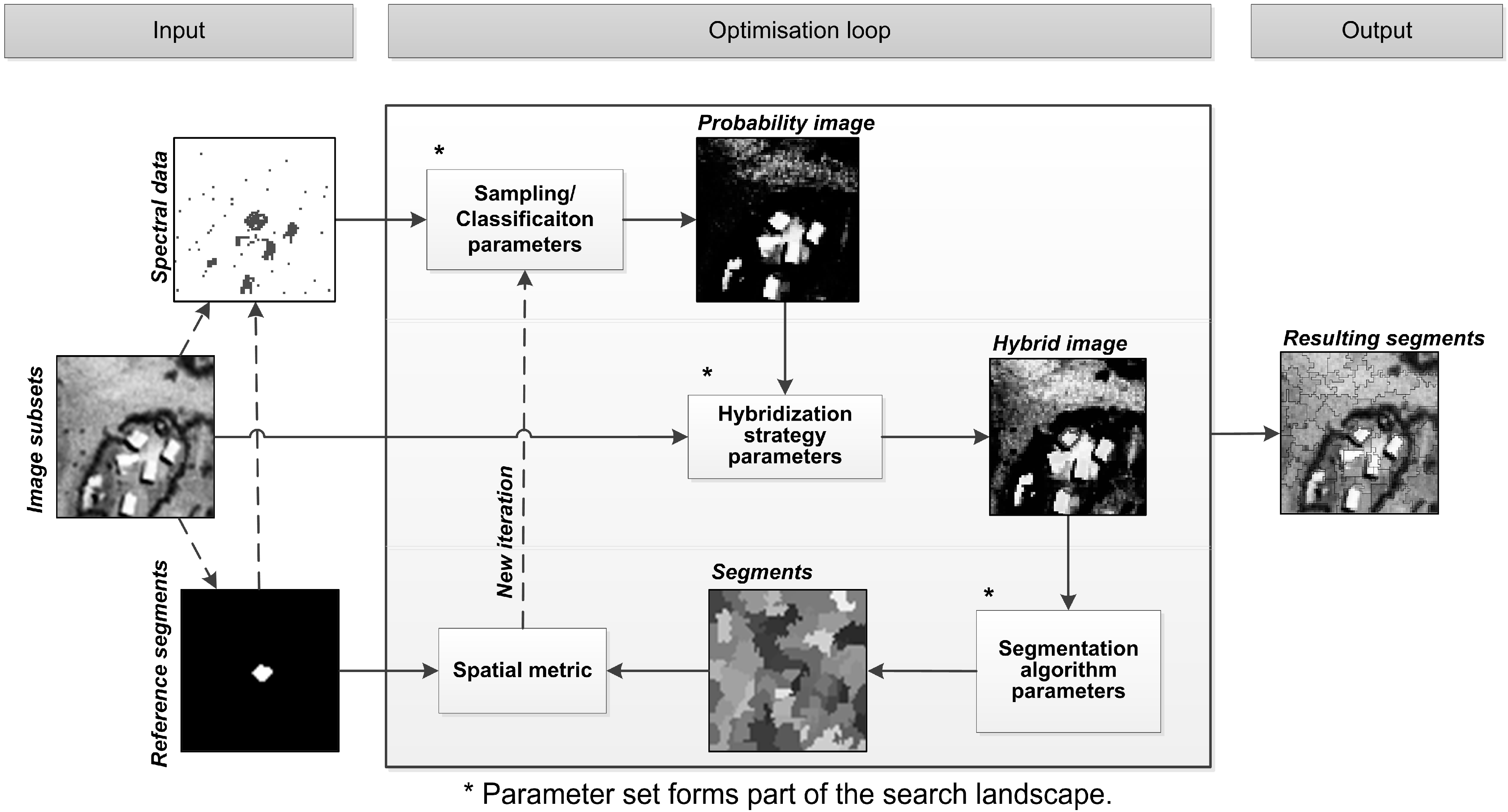
The search landscape may also be extended to include processes surrounding the core segmentation that may lead to better quality segments or classification results [29,45,48]. A search landscape defines the n-dimensional surface of discrepancy metric results for all parameter value combinations, where n is the number of parameters in the method. Additional processes may tailor the data to allow a given segmentation algorithm to perform better, for example by adding extra data transformation functions [29], or by automatically performing post segmentation processes to further improve results. Such processes may be interdependent [52] with segment generation and should subsequently be optimized simultaneously or interdependently with the segmentation algorithm parameters.

3. Classifier Directed Data Hybridization

3.1. Exploiting Spectral Data Contained within Provided Reference Segments for Segment Generation

Reference segment geometric properties are most commonly queried to drive the search process in sample supervised segment generation approaches [26,27,28]. Such reference segments also contain or encapsulate spectral data, which is implicitly provided. Figure 2 illustrates the two basic properties or aspects derived from provided reference segments. The question is raised and explored how the spectral data contained within the provided reference segments (Figure 2. Arrow B) may contribute to generating more accurate image segments (Figure 2. Arrow A) via data modification processes (Figure 2. Arrow C).

Figure 2. The rationale behind the proposed method. Segment geometry is commonly provided via digitizing and used to drive a parameter search process (Arrow A) for segment generation. Reference segment spectral content (Arrow B), which is implicitly provided, is queried to influence a data transformation (Arrow C) affecting segment generation.

Figure 2. The rationale behind the proposed method. Segment geometry is commonly provided via digitizing and used to drive a parameter search process (Arrow A) for segment generation. Reference segment spectral content (Arrow B), which is implicitly provided, is queried to influence a data transformation (Arrow C) affecting segment generation.

It is suggested that pixel based classification methods, although having their limitations compared to object-based image analysis approaches [1], provide useful information in clustering thematic elements in imagery in many instances. Classification in this context is used to assist in segmentation and not for thematic element identification. It is proposed to interleave classification and segmentation processes via an expanded search landscape in the context of sample supervised segment generation. This proposition is inspired by methods that interleave classification and segmentation for thematic element identification purposes [23,53,54,55] and methods defining expanded search landscapes in sample supervised segment generation [29,45]. The spatial/spectral aggregation of segmentation is complimented with the discriminative power of a classification process. Classification is used to tailor the data, so that the given segmentation algorithm performs better. One-class classifiers or novelty detectors having strong discriminative power such as a one-class Support Vector Machine (SVM) [56]/support vector domain descriptor [57] and others [58], may be employed to generate a preliminary classification or probability image (with additional processes, described below) of pixel membership based on the spectral content encapsulated within provided reference segments. Such an initial classification may provide useful information in describing thematic and spectral similarities that may assist in segmentation. On the other hand, it is possible that such information may be detrimental to subsequent segmentation processes, a scenario that may be found in the context of VHR optical data. An example could be accurately segmenting all cars in a parking lot, with the large variation in spectral content causing problems for such a method. Many method variants are possible based on this basic idea. A specific formulation is presented below.

3.2. Method Overview

Figure 3 (source: illustrated abstract, [30]) illustrates the architecture of the proposed method variant. As with the generic formulation of such an approach (Figure 1), a user provides a set of reference segments as input (multiple reference segments). In this variant, the spectral data of the provided reference segments are also collected. This variant requires the same amount of user interaction, and from a user’s perspective requires no additional operations compared to the generic formulation.

Figure 3. Architecture of the variant of sample supervised segment generation incorporating classifier directed data hybridization [30].

Figure 3. Architecture of the variant of sample supervised segment generation incorporating classifier directed data hybridization [30].

The optimization loop contains three sub-components controlled by three real-valued parameter sets. Firstly the provided spectral data are used in a synthetic sample generation and classification process to generate a probability image, detailed in Section 3.3. In this implementation this sub-component is controlled with four real valued parameters. Secondly, the generated probability image is fused or hybridized with the original input image. Four strategies are investigated, detailed in Section 3.4, including only using the probability image for segmentation purposes. This sub-component is controlled by a variable number of parameters, depending on the implementation details (between zero and four). In the third sub-component in the search process, the hybridized image is segmented with a given segmentation algorithm (algorithms detailed in Section 3.5). The segmentation results are evaluated with spatial metrics against the user provided reference segments (detailed in Section 3.6), with the evaluation result passed on to the optimizer (optimizers detailed in Section 3.6), which subsequently initiates a new iteration of the search process. In this implementation the method terminates when 2000 search iterations have passed, which was found a sufficient number of runs in preliminary experimentation and in related work [29,43]. Other termination conditions may be considered.

Figure 4 illustrates an example encoding of a search landscape defined in the method. The optimizer considers probability sampling and classification parameters for probability image generation, image hybridization process control parameters and segmentation algorithm parameters. This results in search landscape dimensions ranging from six to eleven, depending on implementation details. Integer/discrete parameters are converted to real. Example parameter encodings are also illustrated for each sub-component (detailed in following sections). Parameter domain interdependencies are demonstrated in the results section, necessitating the creation of such enlarged search spaces.

Figure 4. An example parameter set, forming the search landscape with interdependent real-valued parameter domains [30].

Figure 4. An example parameter set, forming the search landscape with interdependent real-valued parameter domains [30].

The method was implemented as a graphical user interface driven application programmed in C++, making use of various open source libraries (in acknowledgements). Examining the progress of the automatic parameter tuning process and manually overriding proceedings are possible. Due to the envisaged usage scenario of such an approach, the method is embedded in an exemplary larger workflow containing basic scene wide segmentation and one-class classification functionality.

3.3. Search Landscape: Sampling/Classification Sub-Component

The sampling and classification sub-component entails the parameterization of the process of probability image generation. This can be implemented in various ways, with varying number of parameters and resultant search landscape characteristics. Parameter controlled variation in output is conjectured be most useful. This process is implemented here as follows:

A one-class SVM [56] with a Radial Basis Function (RBF) kernel is run on the spectral samples (normalized) collected from within all provided reference segments. Figure 5a illustrates a subset of a three-band VHR optical image where the aim would be to accurately segment all bright sink roofed structures. The sloped roofs appear spectrally diverse due to the different light reflectance angles. The red polyline in Figure 5a illustrates one of the digitized reference segments or objects provided by a user. This classification process is controlled by two real valued parameters (nu and gamma, see [56] for details).

Figure 5. Image processing conducted to derive a probability image. (a) Illustrates a subset with a delineated reference segment; (b) the masking and synthetic sampling procedure and (c) the generated probability image.

Figure 5. Image processing conducted to derive a probability image. (a) Illustrates a subset with a delineated reference segment; (b) the masking and synthetic sampling procedure and (c) the generated probability image.

This initial classification is used as a mask to prevent the automatic selection or querying of pixels, representing a synthetic secondary class. Figure 5b illustrates blue shaded pixels, which constitute the classification result of the one-class classification process that acts as a mask. The red pixels represent samples taken from a linked list of random samples (generated only once). The red samples match the quantity of pixels found within the reference segments. As the nature of the mask changes (via tuning the parameters of the one-class SVM), some samples selected for the synthetic secondary class may be masked out and new samples are placed, taken from samples in the linked list. In other words, the parameters of the one-class SVM control the pixel sampling (red pixels) of a synthetic secondary class via the creation of a mask (blue pixels).

Subsequently the two sample groups with identical number of pixels are used in a two-class SVM [59] classification process to generate a probability image, illustrated in Figure 5c. The two controlling parameters (C and gamma) are not as sensitive or do not result in significant changes in results compared to the effect of the masking/sampling process. Thus, four parameters control the nature of the probability image, with an optional additional parameter controlling the weight of the interaction in the subsequent process. These parameters encompass the probability image sub-component as illustrated in Figure 3. The parameter range for nu is set to [0, 0.2] and for C and gamma to [0, 100]. Optionally, additional parameters may control the sampling of a synthetic secondary class to create more diversity in the generated probability output. It should be noted that the quality or accuracy of the generated probability imagery is not measured or quantified. Various other implementations are possible.

3.4. Search Landscape: Hybridization Sub-Component

Within the image hybridization sub-component the original input image is modified, guided or directed by the classification results of the probability image. The search process can control the nature and degree of the interaction. This allows for useful aspects to be used from both the imagery. After image segments are generated, the original image should be queried for further image processing and classification processes and not the hybridized image. Three variants of image hybridization are presented and tested. In addition, the probability image itself may be considered for segmentation. Figure 6 illustrates arbitrary results generated by the three variants detailed below. Other variants are possible.

Figure 6. The three variants of data hybridization investigated. (a) Illustrates a hybrid image generated via the (a) band replacement strategy (Section 3.4.1); the (b) move to average strategy (Section 3.4.2) and (c) the move to central positions strategy (Section 3.4.3).

Figure 6. The three variants of data hybridization investigated. (a) Illustrates a hybrid image generated via the (a) band replacement strategy (Section 3.4.1); the (b) move to average strategy (Section 3.4.2) and (c) the move to central positions strategy (Section 3.4.3).

3.4.1. Hybrid:EB (Exchange Band)

The simple Hybrid:EB (Exchange Band) hybridization strategy replaces band x of the input image with the generated probability image (Figure 6a). For experimental conformity all used imagery in this work has three bands, with band two exchanged for the probability image. Simply adding the probability image to the image stack is also possible.

3.4.2. Hybrid:MA (Move to Average)

The Hybrid:MA (Move to Average) strategy (Figure 6b) determines the average spectral value contained in all reference segments. Pixels in the original image (I) are moved towards this position based on the following equation:

$$Hybrid:MA=I-abs\left(I-Avg\right)\times Mag\times Prob-abs\left(I-Avg\right)$$

(1)

where Prob denotes the probability image and Avg the average spectal value, Mag is a user defined value influencing the magnitude of the move (set to two in all experiments) and abs the absolute value. An additional weighting parameter, which forms part of the optimization problem influences the intensities within Prob. Hybrid:MA is thus also a weighted function within the optimization problem. This strategy also allows for pixels to be shifted away from the calculated spectral average. Simply designating the average spectral value of the reference segments as the target spectral position to move pixels towards may be problematic in various problem instances.

3.4.3. Hybrid:CP (Central Positions)

With the Hybrid:CP (Central Positions) hybridization strategy, pixels in the original image are moved towards a parameter controlled new spectral value. The distance of this move (in percentage) is equal to the intensities in the probability image. For each band in the image a parameter is added, thus in this implementation the Hybrid:CP strategy adds an additional three parameters to the optimization problem. When concerned with 8-bit imagery, the parameter range is set to [0, 255]. The intensity of the move is also regulated by a weighting parameter, as with the Hybrid:MA strategy. Hybrid:CP is written as:

$$Hybrid:CP=I-\left(I-CP\right)\times Prob$$

(2)

where I indicates the original input image, CP the parameter controlled spectral position and Prob the probability image as a percentage (when concerned with 8-bit data it would be Prob/255). Figure 6c illustrates an arbitrary hybridized image generated with this strategy. This strategy allows for more flexibility in the hybridization, by allowing the optimizer to define the position where to pixel spectral values should be shifted (at the expense of added search landscape dimensionalities).

3.5. Search Landscape: Segmentation Sub-Component

The hybridized image is passed on to a given segmentation algorithm (Figure 3), where the optimizer also search the parameter space of said algorithm, due to parameter domain interdependencies [29,60]. In this work two segmentation algorithms are tested, namely Multiresolution Segmentation (MS) [12] and Simple Linear Iterative Clustering (SLIC) [61]. The MS algorithm adds an additional three parameters to the search landscape, with a sensitive “scale” parameter majorly responsible for the relative sizes of segments (see [12] for a full formulation). Two other parameters control the influence (Color/Shape) and definition (Compactness/Smoothness) of shape in segment generation. The MS algorithm has been extensively used in the context of GEOBIA [1,2,19,27,46]. Figure 7 illustrates hand tuned results of the MS algorithm run on the original input image (Figure 7a) and on the Hybrid:CP image (Figure 7b) and the SLIC algorithm run on the probability image (Figure 7c).

Figure 7. Segmented subsets, generated with the MS algorithm using the (a) original image, and a (b) Hybrid:CP image and segments generated with SLIC using a (c) probability image.

Figure 7. Segmented subsets, generated with the MS algorithm using the (a) original image, and a (b) Hybrid:CP image and segments generated with SLIC using a (c) probability image.

SLIC, considered a superpixel algorithm, is commonly used in part-based models and non-thematic segmentation tasks (e.g., for purely allowing the extraction of rich attribute sets) [61]. SLIC adds two parameters to the search landscape. Similar to the MS algorithm, SLIC has a “scale” parameter controlling the relative size of generated segments [61]. Although not as efficient as the MS segmentation algorithm for creating thematically accurate segments in a remote sensing context [29], SLIC is computationally efficient allowing for more interactive segment generation in manual tuning processes.

3.6. Metrics and Optimizers

In each iteration of the method, after the image segmentation process, the generated segments are quantitatively compared with the user provided reference segments (Figure 3). Four spatial empirical discrepancy metrics [41] are utilized in experimentation in this work to prevent bias based on the details of any given implementation (segmentation is an ill posed problem [62] due to the variation in possible solutions). Table 1 summarizes the used spatial metrics, with their formulations given using set theory notation. The Reference Bounded Segments Booster (RBSB) [27] compares area offsets between the reference (R) and a generated segment (S). The Larger Segments Booster (LSB) [63] performs similarly, but considers all segments (S_h) having a majority overlap with the reference segment and holds a penalization factor in the form of counting border (b) pixels intersecting the reference segment.

The Partial and Directed Object-Level Consistency Error (PD_OCE) [29,64] and the Reference Weighted Jaccard (RWJ) [29] metrics quantifies quality based on all generated segments intersecting the reference segment, but have a difference based on the importance (area overlap) of generated segments to the problem. The optimal result for all metrics is zero, with the effective range being [0, 1] (with few exceptions). The symbol n denotes the number of generated segments intersecting the given reference segment, while i and j are iterators running through these segments.

Table 1. The four spatial empirical discrepancy metrics used for segment evaluation, written using set theory notation.

Metric	Formulation	Reference
RBSB	$\frac{\left|R{{\displaystyle \cup }}^{\text{}}S\right|-\left|R{{\displaystyle \cap }}^{\text{}}S\right|}{\left|R\right|}$	[27]
LSB	$\frac{\left|R{{\displaystyle \cup }}^{\text{}}{S}_h\right|-\left|R{{\displaystyle \cap }}^{\text{}}{S}_h\right|+b}{\left|R\right|}$	[63]
PD_OCE	${\displaystyle \sum _{i=1}^n}\frac{\left|R{{\displaystyle \cap }}^{\text{}}{S}_i\right|}{\left|R{{\displaystyle \cup }}^{\text{}}{S}_i\right|}\times \frac{\left|S_i\right|}{{{\displaystyle \sum }}_{j=1}^n\left|S_j\right|}$	[64]
RWJ	${\displaystyle \sum _{i=1}^n}\frac{\left|R{{\displaystyle \cap }}^{\text{}}{S}_i\right|}{\left|R{{\displaystyle \cup }}^{\text{}}{S}_i\right|}\times \frac{\left|R{{\displaystyle \cap }}^{\text{}}{S}_i\right|}{\left|R\right|}$	[29]

Table 1. The four spatial empirical discrepancy metrics used for segment evaluation, written using set theory notation.

Metric	Formulation	Reference
RBSB	$\frac{\left|R{{\displaystyle \cup }}^{\text{}}S\right|-\left|R{{\displaystyle \cap }}^{\text{}}S\right|}{\left|R\right|}$	[27]
LSB	$\frac{\left|R{{\displaystyle \cup }}^{\text{}}{S}_h\right|-\left|R{{\displaystyle \cap }}^{\text{}}{S}_h\right|+b}{\left|R\right|}$	[63]
PD_OCE	${\displaystyle \sum _{i=1}^n}\frac{\left|R{{\displaystyle \cap }}^{\text{}}{S}_i\right|}{\left|R{{\displaystyle \cup }}^{\text{}}{S}_i\right|}\times \frac{\left|S_i\right|}{{{\displaystyle \sum }}_{j=1}^n\left|S_j\right|}$	[64]
RWJ	${\displaystyle \sum _{i=1}^n}\frac{\left|R{{\displaystyle \cap }}^{\text{}}{S}_i\right|}{\left|R{{\displaystyle \cup }}^{\text{}}{S}_i\right|}\times \frac{\left|R{{\displaystyle \cap }}^{\text{}}{S}_i\right|}{\left|R\right|}$	[29]

Regarding the optimizers, the “DE/rand/1/bin” variant of the Differential Evolution (DE) [65] metaheuristic is used in this work, based on preliminary experimentation [66] evaluating performances and other published results [29,43] (30 Agents, F = 0.75, CR = 0.3, random positions for initialization). For evaluative purposes, Particle Swarm Optimization (PSO) [67] (30 Agents, Inertia Weight = 0.7, Best Own = 1.5, Best Swarm = 1.5), a Hill Climber (HC) (D = 30) and random sampling (RND) search are also considered [68] in some experiments.

4. Data

The proposed approach is demonstrated and evaluated by generating segments on three VHR optical images. The images depict towns and refugee camps in central and east Africa. The images all contain a single thematic class-of-interest with the elements having varying degrees of thematic and spectral similarities, thus presenting the method with a range of problems in terms of difficulty. The aim is to generate a single segment layer, thematically accurate with respect to the land cover elements of interest. Practically, if segment results are adequate, they may be used as is. Otherwise, it may be considered as an initial segmentation, where additional image processing may be needed (e.g., [14]).

The datasets are named after the settlement of interest in the image. The imagery was fully pre-processed (orthorectified, pansharpened), stretched to 8-bit quantization and subsets were extracted over parts of the settlements. For each site twenty elements are digitized, used as the reference segments. Table 2 lists the metadata and some usage considerations of the three datasets.

Table 2. Metadata of the datasets used.

Test Site	Target Elements	Sensor	Spatial Resolution	Reference Segments	Channels	Date Captured
Bokolmanyo 1	Tents	GeoEye-1	0.5 m	20	1, 2, 3	2011/08/24
Jowhaar 1	Structures	GeoEye-1	1 m *	20	1, 2, 3	2011/02/26
Hagadera 2	Structures	WorldView-2	0.75 m *	20	4, 6, 3	2010/10/07

* Resampled from a 0.5 m spatial resolution. ¹ © GeoEye, Inc. Herndon, VA, USA, 2011, provided by e-GEOS S.p.A. under GSC-DA, all rights reserved. ² © DigitalGlobe, Inc. Longmont, CO, USA, 2010, provided by EUSI under EC/ESA/GSC-DA, all rights reserved.

Table 2. Metadata of the datasets used.

Test Site	Target Elements	Sensor	Spatial Resolution	Reference Segments	Channels	Date Captured
Bokolmanyo 1	Tents	GeoEye-1	0.5 m	20	1, 2, 3	2011/08/24
Jowhaar 1	Structures	GeoEye-1	1 m *	20	1, 2, 3	2011/02/26
Hagadera 2	Structures	WorldView-2	0.75 m *	20	4, 6, 3	2010/10/07

* Resampled from a 0.5 m spatial resolution. ¹ © GeoEye, Inc. Herndon, VA, USA, 2011, provided by e-GEOS S.p.A. under GSC-DA, all rights reserved. ² © DigitalGlobe, Inc. Longmont, CO, USA, 2010, provided by EUSI under EC/ESA/GSC-DA, all rights reserved.

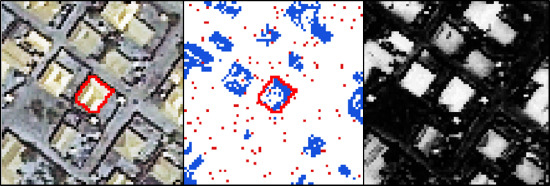
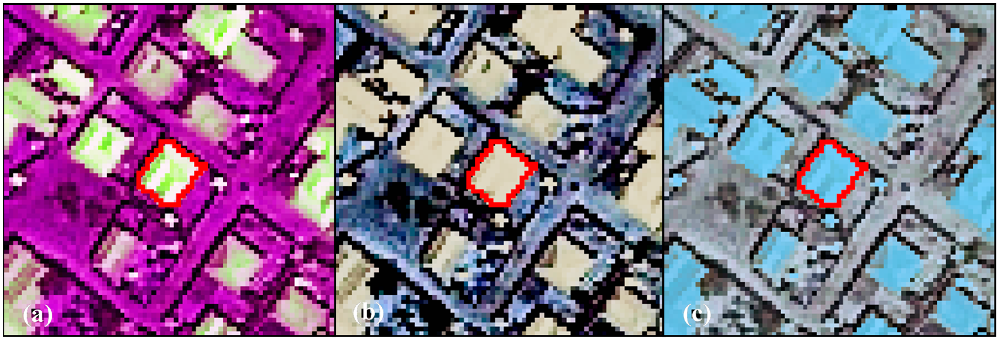
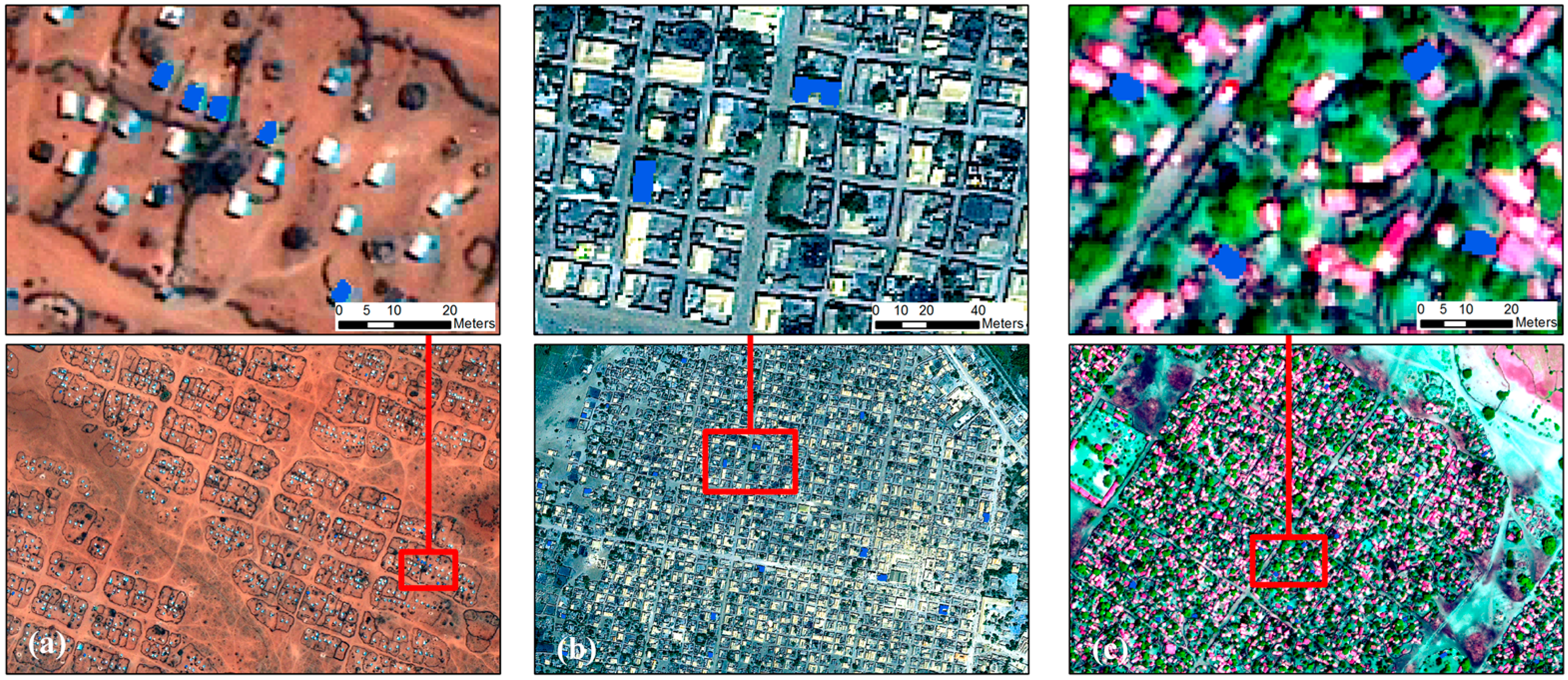
Figure 8. The datasets used for method evaluation, namely (a) Bokolmanyo; (b) Jowhaar and (c) Hagadera. The blue polygons in the enlarged subsets represent digitized reference segments.

Figure 8. The datasets used for method evaluation, namely (a) Bokolmanyo; (b) Jowhaar and (c) Hagadera. The blue polygons in the enlarged subsets represent digitized reference segments.

Figure 8 shows the three image datasets, or problem instances, along with an enlargement over a small area illustrating the characteristics of the elements of interest. The Bokolmanyo site (a) constitutes an easier problem, where the elements of interest are nylon tents in a refugee camp. A thematic segmentation using the SLIC algorithm would be the aim using this image. The other two datasets, Jowhaar (b) and Hagadera (c), contain more divergence in spectral and thematic correlations of the elements of interest. The MS algorithm is used on these datasets. The aim on these two datasets would be to correctly segment all corrugated iron/steel roofed buildings.

5. Experimental Design

The described method (Figure 3) variants are evaluated based on performances compared to the generic formulation (Figure 1) of sample supervised segment generation. Various behavioral characteristics of the method are also quantified, related to the search progression, the feasibility of using different search methods and parameter domain interdependencies. Thus, a comparative experimentalism [66,69] is performed on problem specific datasets.

Due to uncertainty or randomness in terms of sampling (randomly initiated linked list) and classification, metaheuristic progression (initialization, stochastic nature) and segmentation algorithm seeding, multiple runs for experiments are advocated. Results are not specific and have some variation. None the less, in initial experimentation the variance of distributions of results are similar to other work in the context of enlarged search landscapes [29], with statistically significantly different (student’s t-test and Friedman rank test with Nemenyi post hoc test) results observed on relatively small and large preliminary experimental test sets.

5.1. Segment Quality Comparison and Method Ranking

The generic formulation of sample supervised segment generation, the proposed variant using probability images for segmentation and three variants conducting image hybridization, namely Hybrid:EB, Hybrid:MA and Hybrid:CP, are quantitatively compared in terms of resultant segment quality. For each test site (Bokolmanyo, Jowhaar and Hagadera) all the method variants are run using the 20 provided reference segments and selected segmentation algorithm (SLIC for Bokolmanyo and MS for Jowhaar and Hagadera). Experimentation is conducted with the four metrics listed in Table 1. In total, results are reported with 60 different experimental instances (combinations of methods, problem instances and metrics).

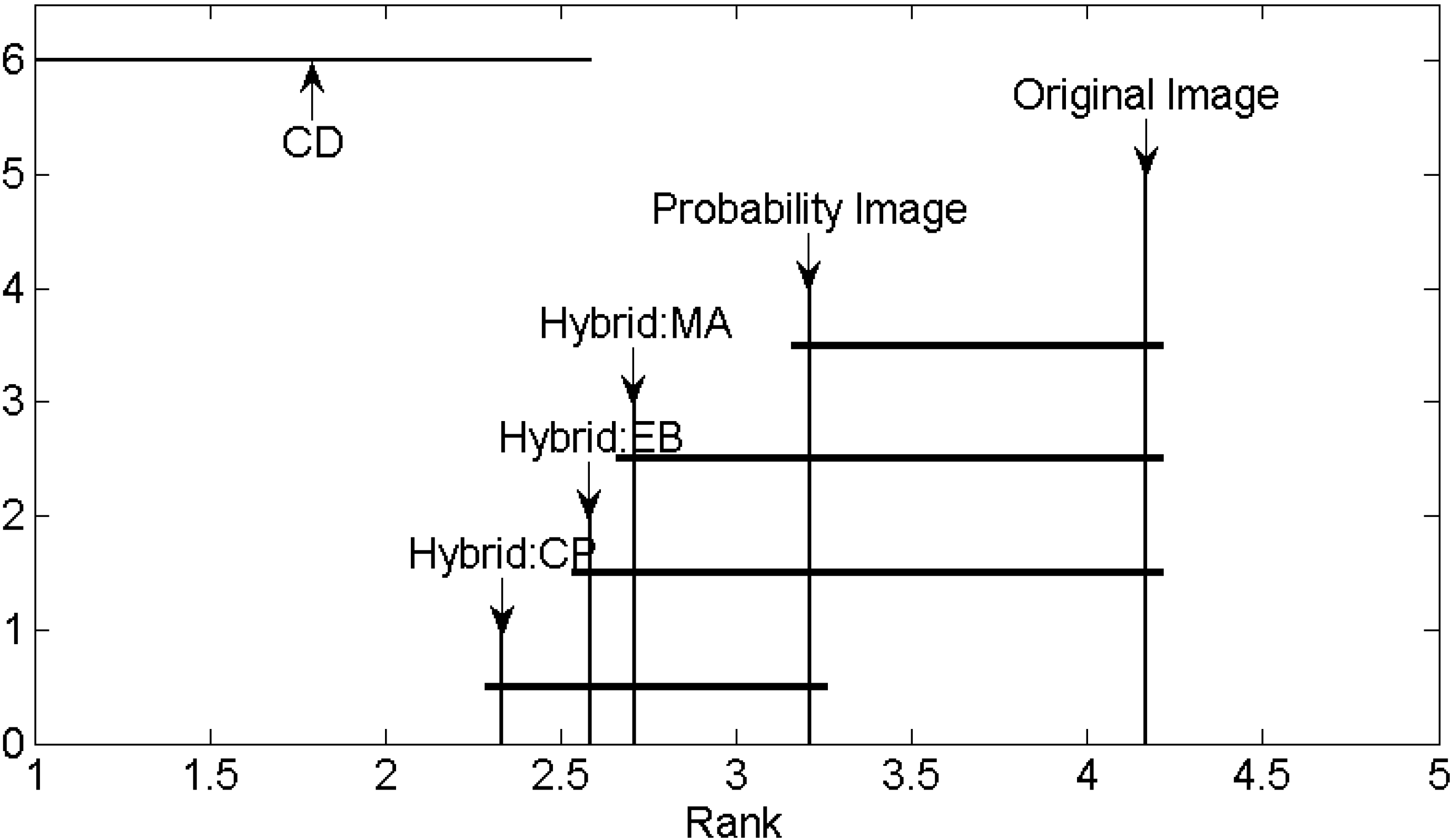
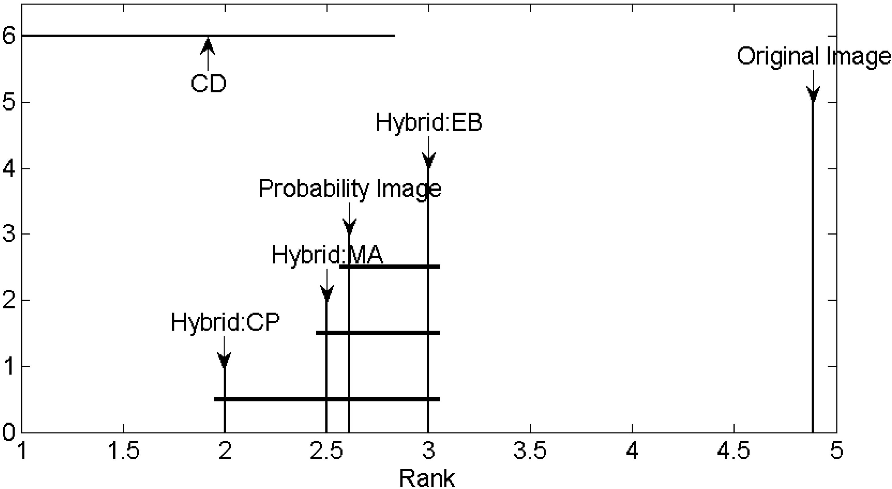
Experimental instances are repeated ten times with the averages, standard deviations and best results achieved reported. Each run consists of 2000 search method iterations using the DE metaheuristic, evaluating the 20 reference structures and taking the mean as the result. In total 24 million segmentation evaluations are performed over the 60 experimental instances. In addition to reporting and discussing the tabularized results, a Friedman test is conducted with a Nemenyi post hoc test [70] to rank the methods and describe their critical differences under all metric and problem type conditions. This is done to give some measure of generalizability [71,72] (commonly done when evaluating multiple classifiers over multiple problem instances), although problem instances and experimental variations are not exhaustive.

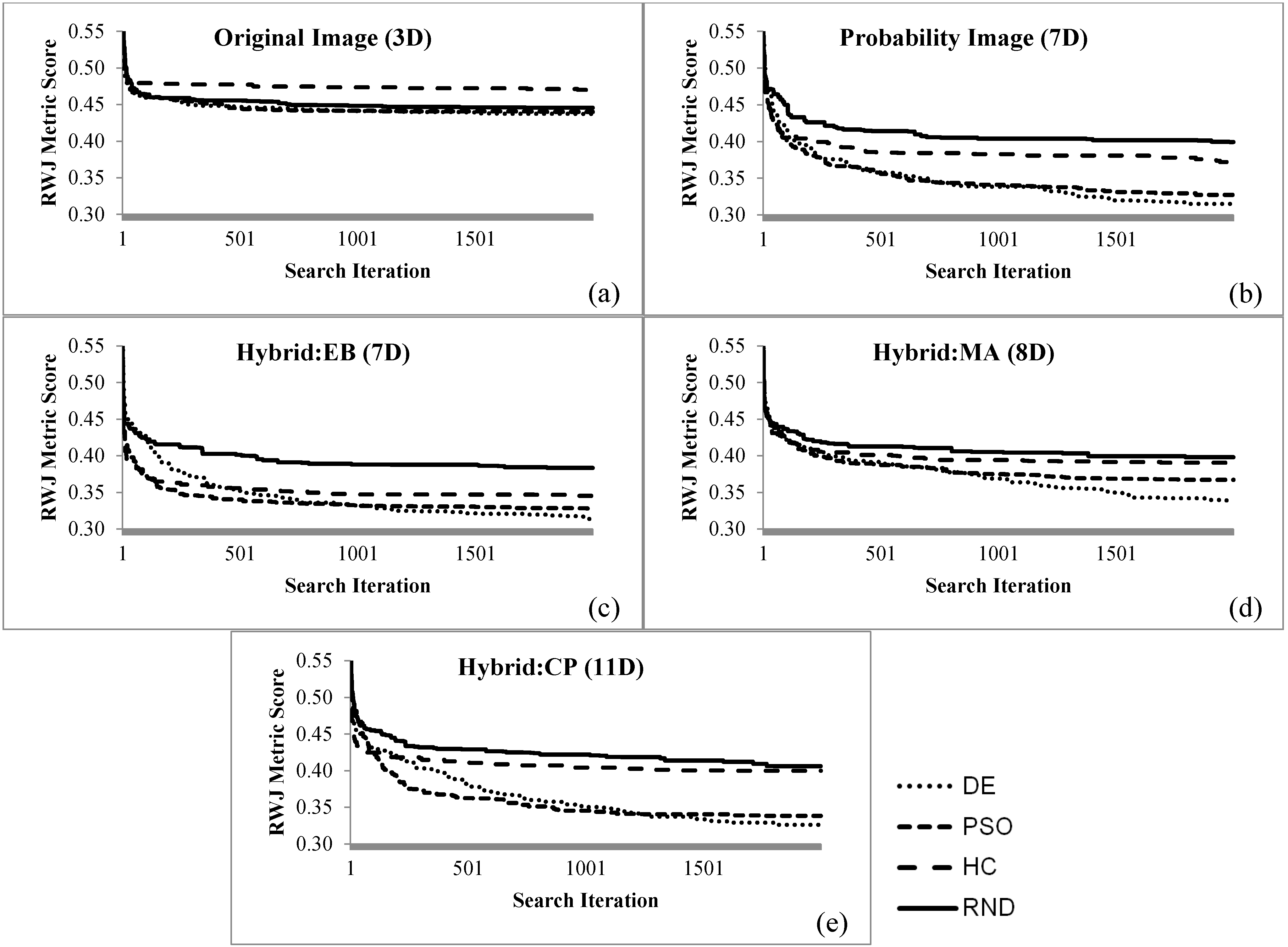
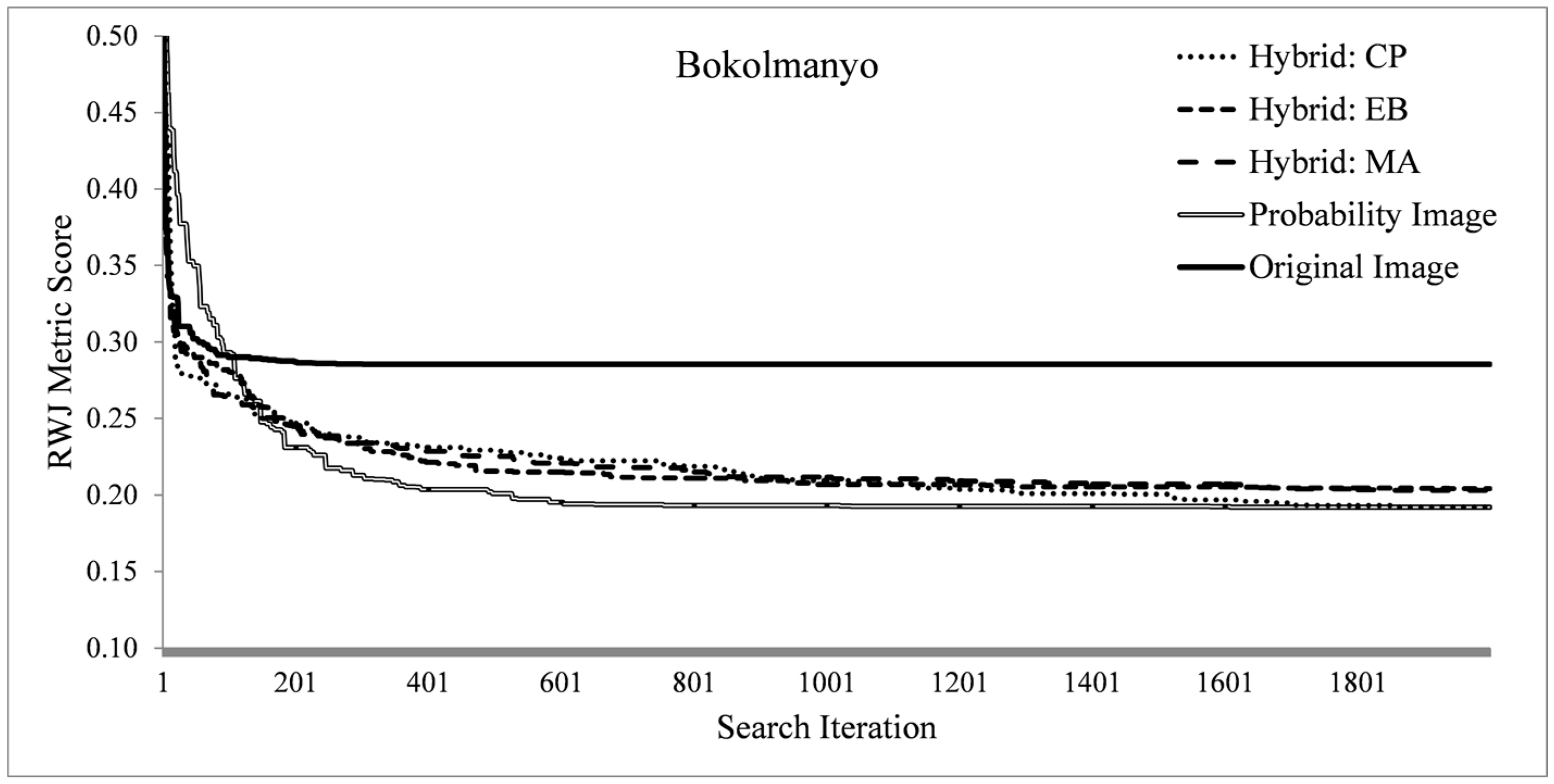
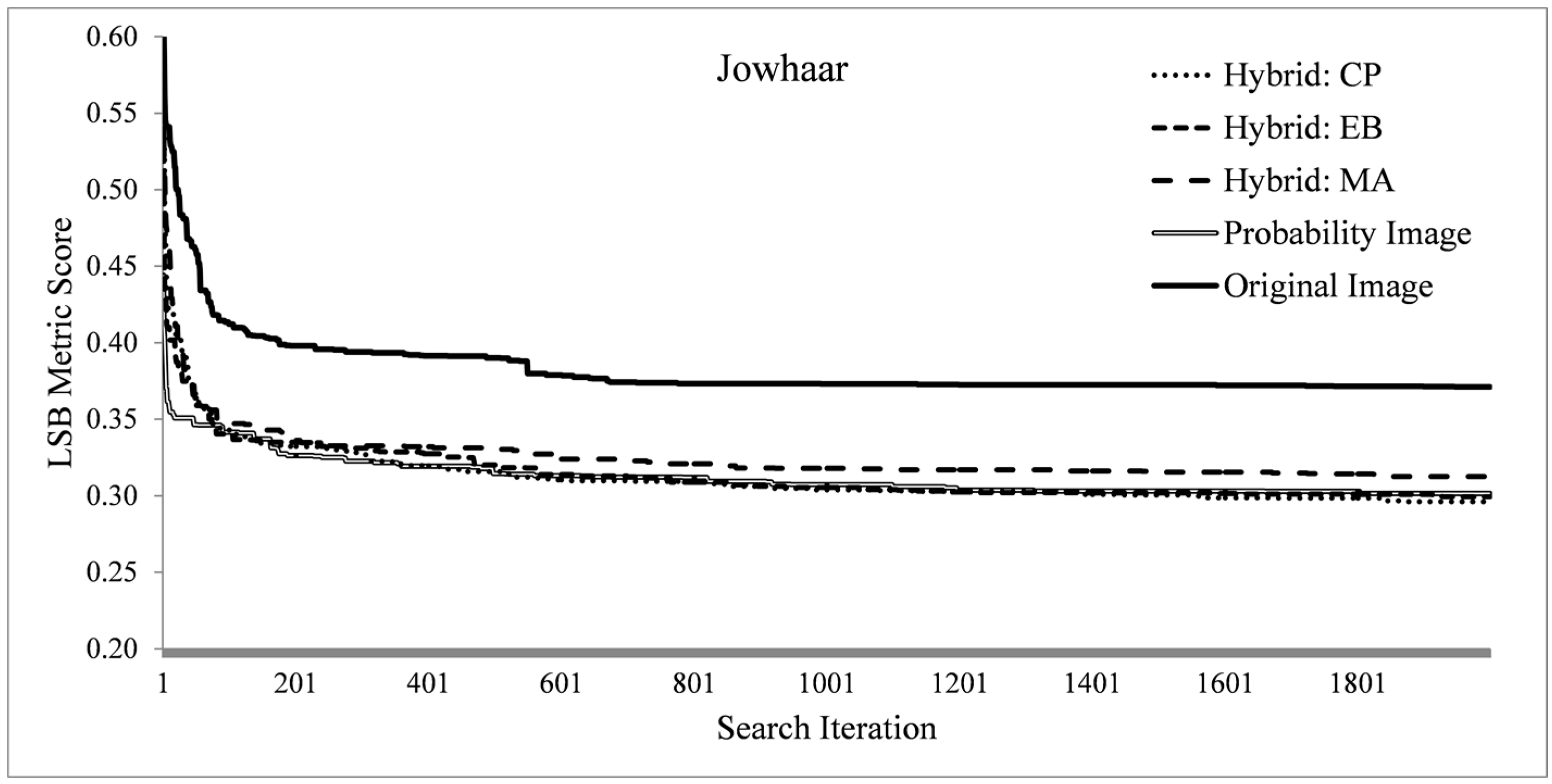
5.2. Search Process Characteristics

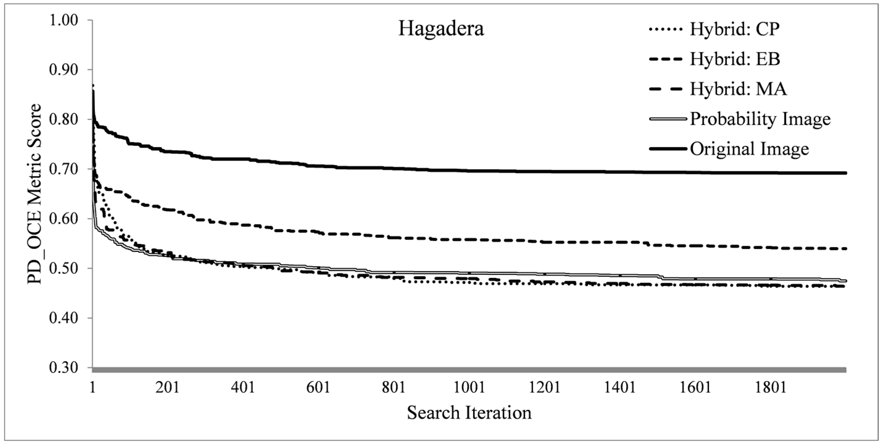
The search process is profiled over the three problem instances by recording the fitness traces over all method variants. It is investigated if the higher dimensional formulations of method variants have any significantly different search profiles. Such search-based methods should terminate as quickly as possible (computationally expensive), thus insight in the search progression is beneficial. For each problem instance a metric is selected, RWJ for Bokolmanyo, LSB for Jowhaar and PD_OCE for Hagadera, and the best metric scores (fitness) are plotted at each of the 2000 method iterations. This diversity in experimentation is introduced as a specific metric or segmentation algorithm (search landscape) might generate bias for a specific hybridization strategy.

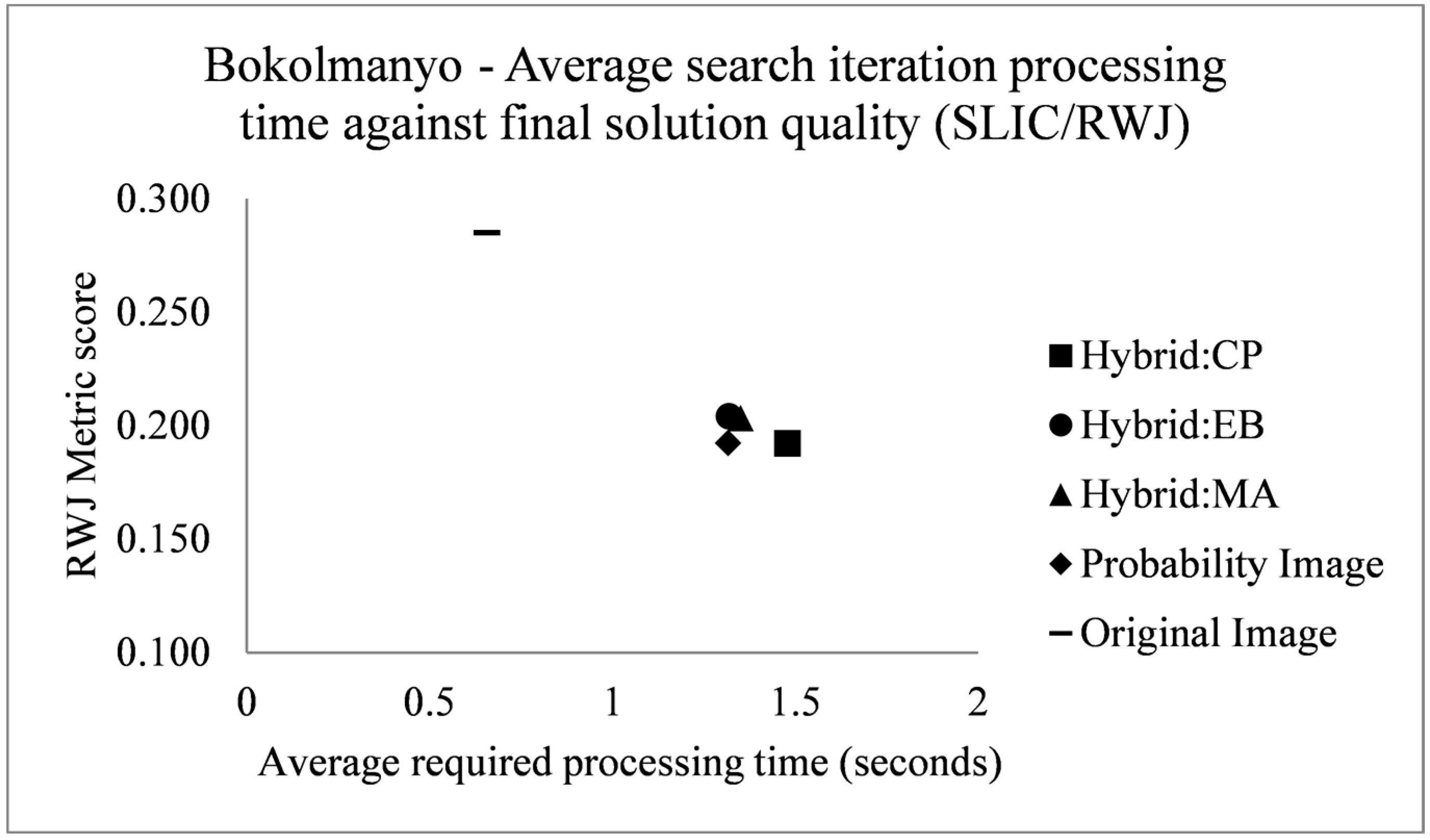
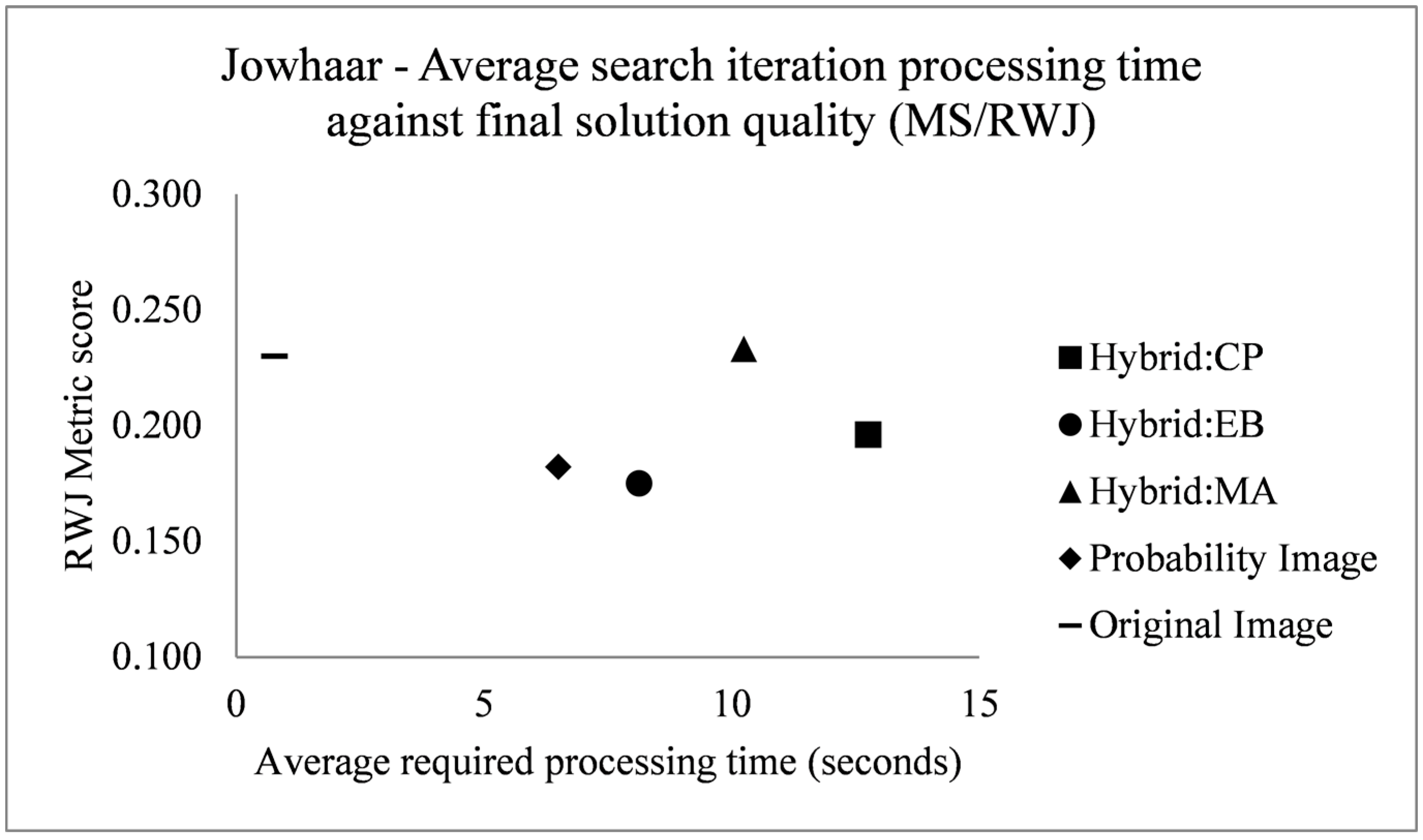
The fitness profiles are supplemented with a profiling of the required computing time of single fitness evaluations or iterations of the search process. This gives an indication, in the investigated problem contexts and utilized computer (Intel Xeon E5-2643 3.5 GHz processor with single core processing), of the required computing time to achieve optimal or near optimal results. For the Bokolmanyo and Jowhaar sites, average required computing time per evaluation is recorded and averaged over 100 iterations for all five method variants. Results are plotted against optimal achieved metric scores (2000 iterations) of the RWJ metric.

5.3. Parameter Interdependencies

It is investigated if parameter domain interdependencies exist between the segmentation and sampling/data hybridization components of the, probability, Hybrid:EB, Hybrid:MA and Hybrid:CP method variants. The utilized segmentation algorithms observe spectral aspects as merging criteria (strongly). Any process performing a modification of the spectral characteristics of the data on which the segmentation algorithms run, will inherently influence the optimal values of the segmentation algorithms’ parameters. Such interdependency requires the simultaneous optimization of data modification and segmentation algorithm parameters, thus leading to optimization problems with enlarged search spaces as opposed to separately solvable problems.

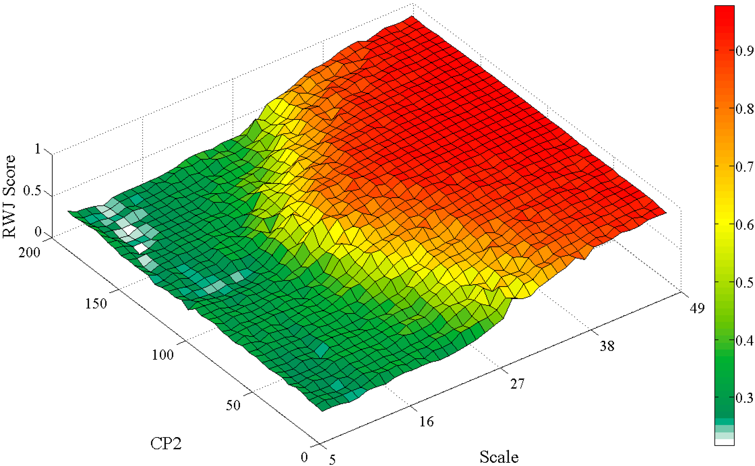
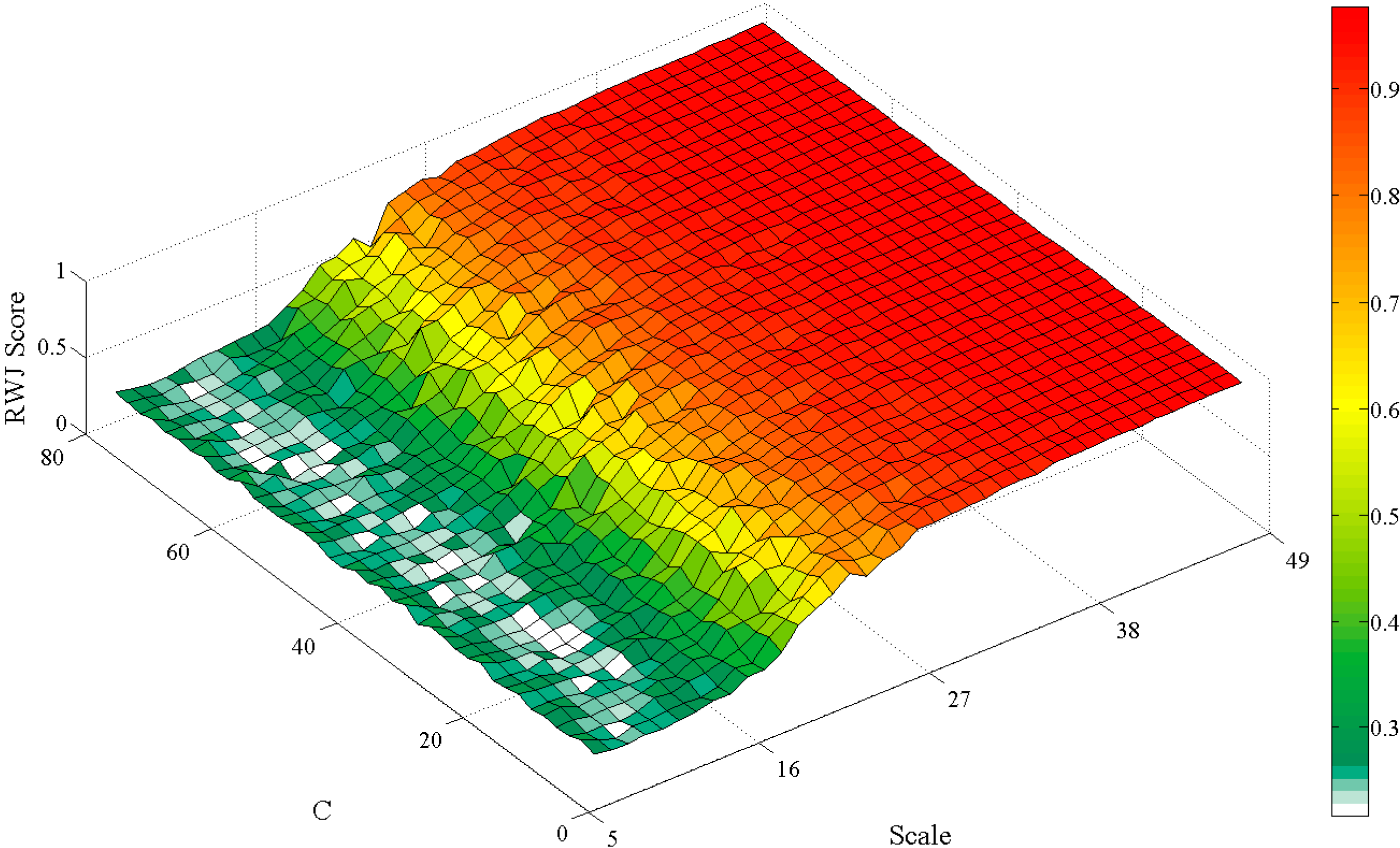
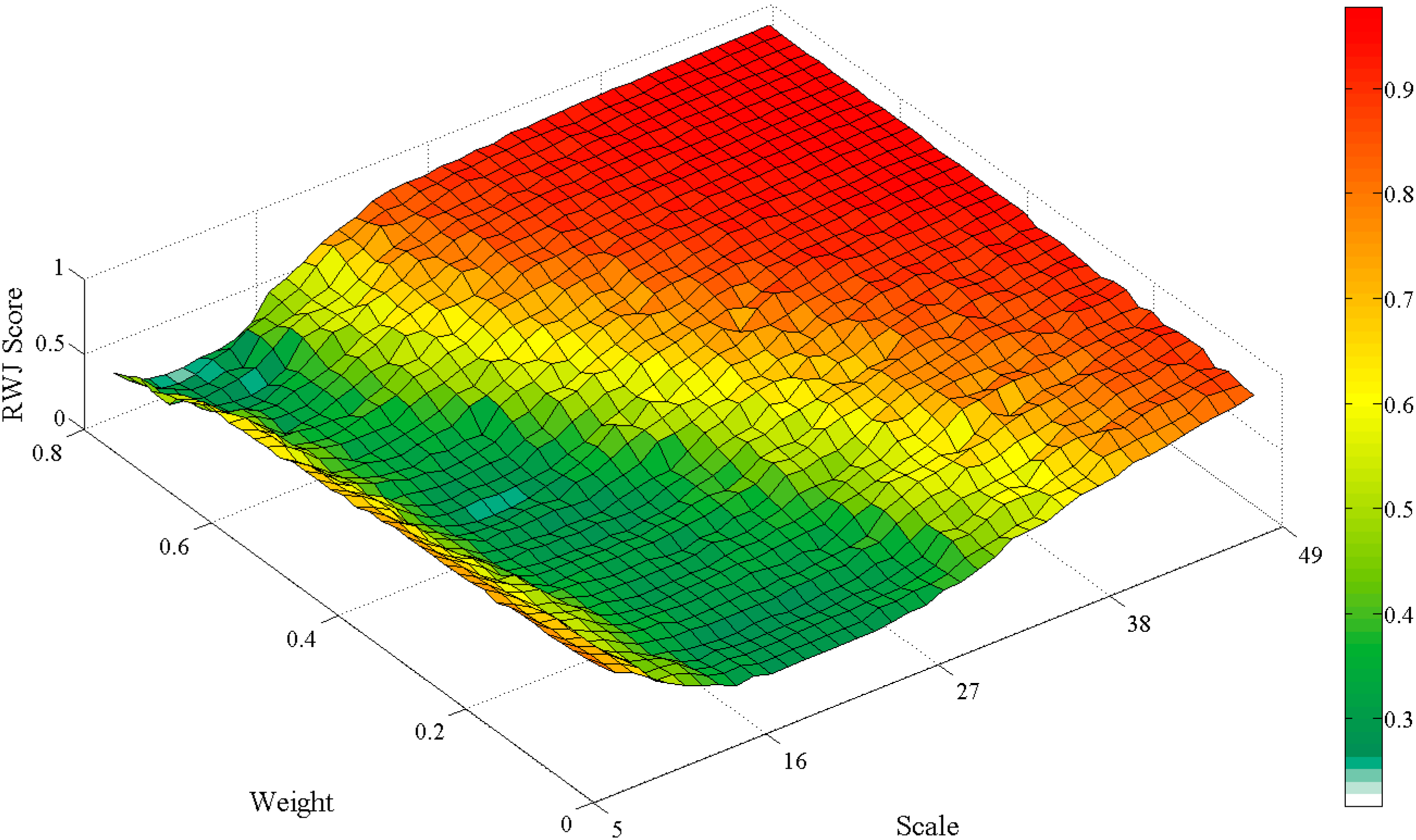
The optimally achieved segmentation algorithm parameters, sampling and classification parameters and the probability weighting parameter are recorded for experimental runs (2000 search iterations, averaged over ten runs) using the five method variants on the three problem instances considering the RWJ metric. The resultant sensitive “scale” parameters of the SLIC and MS segmentation algorithms, considering the proposed method variants, are specifically compared to the resultant parameters considering the generic variant of the method. A student’s t-test is performed to determine if differences are present. Three select two dimensional search surface combinations are also plotted (exhaustive fitness calculations) to visually check for, and demonstrate parameter interdependencies, specifically how the MS scale parameter interact with other parameters of the Hybrid:CP method variant in the Jowhaar problem instance.

5.4. Metaheuristic Viability

Finally the value of using metaheuristics, as opposed to simpler search strategies, is investigated. Simpler search strategies are easier to implement and requires less tuning and would be preferred if metaheuristics provide little performance benefit. It is also investigated how the problem dimensionality (different method variants) affects different search strategies. For one problem instance (Hagadera, MS, RWJ, 2000 iterations, averaged over ten runs) each method variant is run using four different search methods, namely DE, PSO, HC and RND under identical conditions (Section 3.6). The metaparameters for DE and PSO were hand-tuned (meta-optimization could be considered). Fitness traces are plotted to contrast search progress and general performances under these different search landscape conditions. Final optimal achieved metric scores are reported.

6. Results and Discussions

6.1. Segment Quality Comparison and Method Ranking

Table 3, Table 4 and Table 5 lists the results of the metric scores achieved for the three problem instances. The averages and standard deviations are listed. The columns depict method variants and the rows the utilized metrics. Shaded cells highlight the best performing method variants under each metric condition.

Table 3. Segmentation accuracies achieved in the Bokolmanyo problem instance. The shaded cells highlight the results of the best performing hybridization strategy.

Boko (SLIC)		Generic	Probability	Hybrid:EB	Hybrid:MA	Hybrid:CP
LSB	Average	0.544 ± 0.007	0.499 ± 0.036	0.518 ± 0.038	0.482 ± 0.032	0.500 ± 0.075
	Best	0.536	0.416	0.480	0.454	0.426
PD_OCE	Average	0.718 ± 0.000	0.445 ± 0.094	0.538 ± 0.029	0.358 ± 0.038	0.371 ± 0.038
	Best	0.718	0.367	0.486	0.309	0.318
RBSB	Average	0.177 ± 0.008	0.241 ± 0.101	0.189 ± 0.057	0.227 ± 0.044	0.193 ± 0.033
	Best	0.175	0.140	0.145	0.170	0.163
RWJ	Average	0.285 ± 0.006	0.192 ± 0.012	0.204 ± 0.019	0.203 ± 0.017	0.192 ± 0.012
	Best	0.280	0.181	0.190	0.183	0.171

Table 3. Segmentation accuracies achieved in the Bokolmanyo problem instance. The shaded cells highlight the results of the best performing hybridization strategy.

Boko (SLIC)		Generic	Probability	Hybrid:EB	Hybrid:MA	Hybrid:CP
LSB	Average	0.544 ± 0.007	0.499 ± 0.036	0.518 ± 0.038	0.482 ± 0.032	0.500 ± 0.075
	Best	0.536	0.416	0.480	0.454	0.426
PD_OCE	Average	0.718 ± 0.000	0.445 ± 0.094	0.538 ± 0.029	0.358 ± 0.038	0.371 ± 0.038
	Best	0.718	0.367	0.486	0.309	0.318
RBSB	Average	0.177 ± 0.008	0.241 ± 0.101	0.189 ± 0.057	0.227 ± 0.044	0.193 ± 0.033
	Best	0.175	0.140	0.145	0.170	0.163
RWJ	Average	0.285 ± 0.006	0.192 ± 0.012	0.204 ± 0.019	0.203 ± 0.017	0.192 ± 0.012
	Best	0.280	0.181	0.190	0.183	0.171

Table 4. Segmentation accuracies achieved in the Jowhaar problem instance. The shaded cells highlight the results of the best performing hybridization strategy.

Jowhaar (MS)		Generic	Probability	Hybrid:EB	Hybrid:MA	Hybrid:CP
LSB	Average	0.371 ± 0.006	0.302 ± 0.008	0.299 ± 0.007	0.313 ± 0.005	0.296 ± 0.014
	Best	0.361	0.295	0.285	0.307	0.281
PD_OCE	Average	0.581 ± 0.010	0.413 ± 0.034	0.434 ± 0.024	0.361 ± 0.034	0.315 ± 0.040
	Best	0.558	0.382	0.409	0.301	0.261
RBSB	Average	0.187 ± 0.008	0.223 ± 0.091	0.184 ± 0.045	0.207 ± 0.018	0.201 ± 0.030
	Best	0.180	0.118	0.141	0.182	0.170
RWJ	Average	0.230 ± 0.004	0.182 ± 0.032	0.175 ± 0.018	0.233 ± 0.037	0.196 ± 0.029
	Best	0.225	0.145	0.138	0.182	0.159

Table 4. Segmentation accuracies achieved in the Jowhaar problem instance. The shaded cells highlight the results of the best performing hybridization strategy.

Jowhaar (MS)		Generic	Probability	Hybrid:EB	Hybrid:MA	Hybrid:CP
LSB	Average	0.371 ± 0.006	0.302 ± 0.008	0.299 ± 0.007	0.313 ± 0.005	0.296 ± 0.014
	Best	0.361	0.295	0.285	0.307	0.281
PD_OCE	Average	0.581 ± 0.010	0.413 ± 0.034	0.434 ± 0.024	0.361 ± 0.034	0.315 ± 0.040
	Best	0.558	0.382	0.409	0.301	0.261
RBSB	Average	0.187 ± 0.008	0.223 ± 0.091	0.184 ± 0.045	0.207 ± 0.018	0.201 ± 0.030
	Best	0.180	0.118	0.141	0.182	0.170
RWJ	Average	0.230 ± 0.004	0.182 ± 0.032	0.175 ± 0.018	0.233 ± 0.037	0.196 ± 0.029
	Best	0.225	0.145	0.138	0.182	0.159

Table 5. Segmentation accuracies achieved in the Hagadera problem instance. The shaded cells highlight the results of the best performing hybridization strategy.

Hagadera (MS)		Generic	Probability	Hybrid:EB	Hybrid:MA	Hybrid:CP
LSB	Average	0.628 ± 0.005	0.564 ± 0.030	0.549 ± 0.019	0.525 ± 0.034	0.537 ± 0.018
	Best	0.622	0.532	0.513	0.488	0.512
PD_OCE	Average	0.692 ± 0.028	0.474 ± 0.009	0.540 ± 0.027	0.464 ± 0.014	0.464 ± 0.017
	Best	0.681	0.464	0.501	0.445	0.427
RBSB	Average	0.371 ± 0.010	0.406 ± 0.022	0.330 ± 0.029	0.340 ± 0.057	0.387 ± 0.079
	Best	0.350	0.383	0.276	0.274	0.272
RWJ	Average	0.437 ± 0.007	0.314 ± 0.019	0.313 ± 0.028	0.339 ± 0.029	0.326 ± 0.026
	Best	0.424	0.284	0.286	0.301	0.293

Table 5. Segmentation accuracies achieved in the Hagadera problem instance. The shaded cells highlight the results of the best performing hybridization strategy.

Hagadera (MS)		Generic	Probability	Hybrid:EB	Hybrid:MA	Hybrid:CP
LSB	Average	0.628 ± 0.005	0.564 ± 0.030	0.549 ± 0.019	0.525 ± 0.034	0.537 ± 0.018
	Best	0.622	0.532	0.513	0.488	0.512
PD_OCE	Average	0.692 ± 0.028	0.474 ± 0.009	0.540 ± 0.027	0.464 ± 0.014	0.464 ± 0.017
	Best	0.681	0.464	0.501	0.445	0.427
RBSB	Average	0.371 ± 0.010	0.406 ± 0.022	0.330 ± 0.029	0.340 ± 0.057	0.387 ± 0.079
	Best	0.350	0.383	0.276	0.274	0.272
RWJ	Average	0.437 ± 0.007	0.314 ± 0.019	0.313 ± 0.028	0.339 ± 0.029	0.326 ± 0.026
	Best	0.424	0.284	0.286	0.301	0.293

Firstly, variation is noted in which method variants perform best under different metric conditions, justifying an investigation using multiple metrics. The use of a single quality metric would create bias. The magnitude of differences also varies, depending on the metric used and the problem instance. Very small standard deviations in results are observed when considering the generic formulation of the method, with the variants consisting of enlarged search spaces and containing more stochastic processes displaying larger variation in optimally achieved results. The intensities of the variations are also metric dependent, with the RBSB metric showing the most variation in results. It is conjectured that the search surfaces resultant from the RBSB metric (Table 1) creates more irregularities/noise, due to its simpler formulation that only considers a generated segment with the largest overlap with a reference segment.

Considering Table 3, depicting the Bokolmanyo problem instance using the SLIC segmentation algorithm, the Hybrid:MA strategy provided the best segment results when considering the LSB and PD_OCE metrics. The Hybrid:CP strategy performed best when considering the RWJ metric and the generic method variant when considering the RBSB metric. Comparing the generic variant with the proposed variants, substantial improvements in quality is observed under LSB, PD_OCE and RWJ metric conditions.

For the Jowhaar problem instance (Table 4) using the MS segmentation algorithm, the Hybrid:CP (LSB and PD_OCE) and Hybrid:EB (RBSB and RWJ) strategies provided the best results. Again, significant improvements in results are achieved compared to the generic formulation of the method, with results with the RBSB metric the exception. Figure 9 illustrates segmentation results obtained, focused on a single reference structure chosen randomly, under the RWJ metric condition. Note that results are averaged over all provided reference segments, and that the illustrated RWJ scores are segment specific.

Similarly on the Hagadera test site (Table 5), constituting the most difficult problem, the Hybrid:EB, Hybrid:MA and Hybrid:CP method variants produced the best results. Results in this problem instance was generally worse than on the other two datasets, strongly suggesting the use of additional image processing to further process segments. Notwithstanding, significant improvements in results from the hybrid method variants are still useful (much closer to correct). Generally speaking, the proposed method variants have less specific results (more uncertainty) due to the addition of more free parameters and classification processes, but still perform much better than the generic variant in many instances.

Figure 10 illustrates a Nemenyi post hoc test conducted after a Friedman test, ranking the performances of the five investigated method variants based on the 12 experiments (three problem instances and four metrics) conducted with each. The Hybrid:CP strategy performed the best, followed by the other hybridization strategies. The generic formulation of the method (Original Image) is ranked the lowest. A critical difference exist between the Hybrid:CP and the generic method. If the RBSB metric (problematic) is omitted from the test, illustrated in Figure 11, all method variants perform better with a critical difference compared to the generic method. Thus, even with the variation introduced by the metaheuristic and classification, the methods are still useful. The Hybrid:CP strategy is still ranked first. Critical differences are not present among proposed method variants, suggesting a strong dependence on problem conditions and the nature of the metric and the optimal hybridization strategy. Interestingly, segmenting with the probability image is ranked better than the Hybrid:EB strategy. This could be different if a different band was replaced or if the probability image was merely added to the image stack.

Figure 9. Segmentation results achieved with the Jowhaar problem instance (MS) using the RWJ metric. The red polyline delineate one of the twenty reference segments (a) provided by a user; (b) Shows results with the generic formulation; (c) using the probability image and the (d) Hybrid:EB; (e) Hybrid:MA and (f) Hybrid:CP strategies. RWJ metric scores for this specific structure are also given.

Figure 9. Segmentation results achieved with the Jowhaar problem instance (MS) using the RWJ metric. The red polyline delineate one of the twenty reference segments (a) provided by a user; (b) Shows results with the generic formulation; (c) using the probability image and the (d) Hybrid:EB; (e) Hybrid:MA and (f) Hybrid:CP strategies. RWJ metric scores for this specific structure are also given.

Figure 10. Nemenyi post hoc test performed after a Friedman test, ranking the different methods over all metric and problem instances. Horizontal lines indicate the Critical Differences (CD).

Figure 10. Nemenyi post hoc test performed after a Friedman test, ranking the different methods over all metric and problem instances. Horizontal lines indicate the Critical Differences (CD).

Figure 11. The Nemenyi post hoc test, with the RBSB metric omitted. Horizontal lines indicate the Critical Differences (CD).

Figure 11. The Nemenyi post hoc test, with the RBSB metric omitted. Horizontal lines indicate the Critical Differences (CD).

6.2. Search Process Characteristics

Figure 12, Figure 13 and Figure 14 illustrate the fitness traces over the three problem instances (averaged over ten runs), specifically, Figure 12 show the fitness traces for the Bokolmanyo problem instance using the RWJ metric, Figure 13 the fitness traces for the Jowhaar problem instance using the LSB metric and Figure 14 the fitness traces for the Hagadera problem instance with the PD_OCE metric.

In all of the problem instances the proposed method variants obtain better results very early on in the search process compared to the generic variant of the method. This can be attributed to the nature of the probability image, which in many cases immediately provides improved results irrespective of how the parameters of the segmentation algorithm are tuned or how the hybridization parameters are tuned.

Observing Figure 12, the low dimensional generic variant of the method (only two dimensions of the parameters of the SLIC segmentation algorithm), obtains its best fitness extremely early on in the search process, at around 200 fitness evaluations. All other method variants already provide better fitness at this mark, with optimal results achieved near the 1000 iteration mark. Thus, the simpler, lower dimensional method variants have no initial advantage over the more elaborate method variants, suggesting no penalties in terms of search iterations. In this specific instance, only the probability image variant lags slightly behind the generic variant.

Figure 13 and Figure 14 (MS segmentation) have similar profiles, with the proposed method variants outperforming the generic variant in terms of fitness throughout the search process. Interestingly, all four variants have very similar fitness profiles, with the exception of the Hybrid:MA strategy on the Hagadera problem instance. These results suggest the proposed method variants obtain better results faster, even though their search landscape dimensionalities are higher. Under these experimental conditions, 1000 search iterations seem sufficient for the methods to obtain their optimal results, which parallels with results reported elsewhere [29,43], even though search landscapes may have different characteristics.

Figure 12. Fitness traces for the Bokolmanyo problem instance.

Figure 12. Fitness traces for the Bokolmanyo problem instance.

Figure 13. Fitness traces for the Jowhaar problem instance.

Figure 13. Fitness traces for the Jowhaar problem instance.

Figure 14. Fitness traces for the Hagadera problem instance.

Figure 14. Fitness traces for the Hagadera problem instance.

Figure 15 and Figure 16 illustrate the search iteration execution times for the Bokolmanyo (Figure 15) and Jowhaar (Figure 16) problem instances. A single search method evaluation instance (fitness evaluation) encompasses segmenting 20 image subsets (around the reference segments) and comparing the generated segments with that of the reference segment using a given metric. With the proposed method variants, sampling, classification and image hybridization processes are added. Results are averaged over 100 runs.

Figure 15. Search iteration execution time profiling for the Bokolmanyo problem instance.

Figure 15. Search iteration execution time profiling for the Bokolmanyo problem instance.

Figure 16. Search iteration execution time profiling for the Jowhaar problem instance.

Figure 16. Search iteration execution time profiling for the Jowhaar problem instance.

The original variant of the method takes around 0.5 s to complete a single evaluation in both problem instances. In the context of the Bokolmanyo problem instance the proposed method variants needs about three times longer to execute. The majority of the time is taken by the masking process (computational profiling), specifically the libSVM [73] predict function and to a lesser extent the two-class probability image classification process. As the number of support vectors increase, so do the required computing time to determine the label of a new pixel under consideration.

Figure 16 shows a similar characteristic, but with lengthier execution times and more variation depending on the method variant used. Such variation can be explained by the nature of the probability image that was found most useful, having varying numbers of support vectors (and thus increasing the time required to predict pixel values). Alternative classifiers, which predict faster, may be considered to alleviate the increase in required computing times.

6.3. Parameter Interdependencies

Table 6, Table 7 and Table 8 list the average parameter values obtained for the three problem instances. The columns list the segmentation algorithm and probability image generation parameters. “S nu” and “S gamma” are the one-class SVM parameters and “C C” and “C Gamma” the two-class SVM parameters. The rows delineate the method variant under consideration. The shaded cells indicate scale parameters achieved under proposed method variant conditions, which differ from the resultant scale parameter under the generic method variant condition (student’s t-test with a 95% confidence interval). In all but one of the problem instances, with both the SLIC and MS segmentation algorithms, the proposed method variants have statistically significantly different optimal scale parameters compared to the generic method variant. This suggest an influence of probability and hybridization (where applicable) processes on the optimal scale parameter within the given segmentation algorithm.

In the case of the SLIC algorithm (Table 6), very specific optimal scale parameters are generated. In the case of the MS algorithm (Table 7 and Table 8), more diversity is present, with differences (optimal values and standard deviations) attributed to the natures of the different method variants. All the other parameters illustrate extreme variation in optimal results obtained, suggesting multiple combinations of parameters can deliver optimal or near optimal results (within the capability of the method—thus multiple “near global optima” in search landscape terms). This corroborates the importance of the scale parameters with these two segmentation algorithms. The probability image is very beneficial in most cases, with the weighting parameter having relatively high values in most instances.

Table 6. Parameters generated for the Bokolmanyo problem instance.

SLIC/RWJ	Scale	Compactness	S Nu	S Gamma	C C	C Gamma	Weight
Original	9.500 ± 0.745	20.710 ± 3.653	NA	NA	NA	NA	NA
Probability	8.100 ± 1.449	22.360 ± 2.723	0.077 ± 0.086	64.400 ± 34.004	0.002 ± 0.000	48.200 ± 36.715	NA
Hybrid:EB	9.150 ± 0.530	19.180 ± 4.193	0.099 ± 0.077	27.600 ± 38.295	9.800 ± 30.990	47.800 ± 40.524	NA
Hybrid:MA	8.100 ± 2.196	19.120 ± 4.994	0.079 ± 0.090	43.800 ± 37.434	26.600 ± 37.441	47.800 ± 27.848	0.730 ± 0.239
Hybrid:CP	8.700 ± 1.457	23.290 ± 2.388	0.065 ± 0.086	48.800 ± 35.916	39.600 ± 39.764	52.600 ± 33.586	0.664 ± 0.151

Table 6. Parameters generated for the Bokolmanyo problem instance.

SLIC/RWJ	Scale	Compactness	S Nu	S Gamma	C C	C Gamma	Weight
Original	9.500 ± 0.745	20.710 ± 3.653	NA	NA	NA	NA	NA
Probability	8.100 ± 1.449	22.360 ± 2.723	0.077 ± 0.086	64.400 ± 34.004	0.002 ± 0.000	48.200 ± 36.715	NA
Hybrid:EB	9.150 ± 0.530	19.180 ± 4.193	0.099 ± 0.077	27.600 ± 38.295	9.800 ± 30.990	47.800 ± 40.524	NA
Hybrid:MA	8.100 ± 2.196	19.120 ± 4.994	0.079 ± 0.090	43.800 ± 37.434	26.600 ± 37.441	47.800 ± 27.848	0.730 ± 0.239
Hybrid:CP	8.700 ± 1.457	23.290 ± 2.388	0.065 ± 0.086	48.800 ± 35.916	39.600 ± 39.764	52.600 ± 33.586	0.664 ± 0.151

Table 7. Parameters generated for the Hagadera problem instance.

MS/RWJ	Scale	Colour	Compt	S Nu	S Gamma	C C	C Gamma	Weight
Original	17.430 ± 8.200	0.132 ± 0.110	0.514 ± 0.389	NA	NA	NA	NA	NA
Probability	5.990 ± 1.211	0.074 ± 0.081	0.481 ± 0.302	0.060 ± 0.079	40.400 ± 43.090	34.600 ± 40.189	29.400 ± 37.131	NA
Hybrid:EB	8.300 ± 9.334	0.046 ± 0.136	0.219 ± 0.259	0.107 ± 0.082	55.000 ± 25.910	25.400 ± 39.934	37.400 ± 43.950	NA
Hybrid:MA	9.070 ± 10.640	0.068 ± 0.171	0.263 ± 0.253	0.127 ± 0.087	59.000 ± 35.380	22.600 ± 28.316	49.600 ± 34.329	0.772 ± 0.180
Hybrid:CP	5.880 ± 1.623	0.036 ± 0.050	0.442 ± 0.333	0.072 ± 0.078	65.200 ± 43.627	28.200 ± 43.782	60.600 ± 39.090	0.906 ± 0.161

Table 7. Parameters generated for the Hagadera problem instance.

MS/RWJ	Scale	Colour	Compt	S Nu	S Gamma	C C	C Gamma	Weight
Original	17.430 ± 8.200	0.132 ± 0.110	0.514 ± 0.389	NA	NA	NA	NA	NA
Probability	5.990 ± 1.211	0.074 ± 0.081	0.481 ± 0.302	0.060 ± 0.079	40.400 ± 43.090	34.600 ± 40.189	29.400 ± 37.131	NA
Hybrid:EB	8.300 ± 9.334	0.046 ± 0.136	0.219 ± 0.259	0.107 ± 0.082	55.000 ± 25.910	25.400 ± 39.934	37.400 ± 43.950	NA
Hybrid:MA	9.070 ± 10.640	0.068 ± 0.171	0.263 ± 0.253	0.127 ± 0.087	59.000 ± 35.380	22.600 ± 28.316	49.600 ± 34.329	0.772 ± 0.180
Hybrid:CP	5.880 ± 1.623	0.036 ± 0.050	0.442 ± 0.333	0.072 ± 0.078	65.200 ± 43.627	28.200 ± 43.782	60.600 ± 39.090	0.906 ± 0.161

Table 8. Parameters generated for the Jowhaar problem instance.

MS/RWJ	Scale	Colour	Compt	S Nu	S Gamma	C C	C Gamma	Weight
Original	15.890 ± 3.646	0.054 ± 0.023	0.692 ± 0.245	NA	NA	NA	NA	NA
Probability	21.317 ± 3.507	0.146 ± 0.112	0.736 ± 0.225	0.081 ± 0.091	22.000 ± 26.743	40.667 ± 30.820	51.667 ± 23.304	NA
Hybrid:EB	17.571 ± 8.253	0.049 ± 0.045	0.602 ± 0.379	0.096 ± 0.101	57.143 ± 46.056	76.286 ± 12.880	46.571 ± 35.132	NA
Hybrid:MA	27.943 ± 7.056	0.385 ± 0.245	0.762 ± 0.366	0.113 ± 0.084	50.571 ± 40.078	60.000 ± 31.305	44.571 ± 38.587	0.911 ± 0.046
Hybrid:CP	33.600 ± 11.055	0.423 ± 0.293	0.747 ± 0.360	0.118 ± 0.090	42.286 ± 33.950	53.429 ± 28.230	20.857 ± 32.308	0.937 ± 0.068

Table 8. Parameters generated for the Jowhaar problem instance.

MS/RWJ	Scale	Colour	Compt	S Nu	S Gamma	C C	C Gamma	Weight
Original	15.890 ± 3.646	0.054 ± 0.023	0.692 ± 0.245	NA	NA	NA	NA	NA
Probability	21.317 ± 3.507	0.146 ± 0.112	0.736 ± 0.225	0.081 ± 0.091	22.000 ± 26.743	40.667 ± 30.820	51.667 ± 23.304	NA
Hybrid:EB	17.571 ± 8.253	0.049 ± 0.045	0.602 ± 0.379	0.096 ± 0.101	57.143 ± 46.056	76.286 ± 12.880	46.571 ± 35.132	NA
Hybrid:MA	27.943 ± 7.056	0.385 ± 0.245	0.762 ± 0.366	0.113 ± 0.084	50.571 ± 40.078	60.000 ± 31.305	44.571 ± 38.587	0.911 ± 0.046
Hybrid:CP	33.600 ± 11.055	0.423 ± 0.293	0.747 ± 0.360	0.118 ± 0.090	42.286 ± 33.950	53.429 ± 28.230	20.857 ± 32.308	0.937 ± 0.068

Figure 17, Figure 18 and Figure 19 illustrate two dimensional search surface slices obtained with the Jowhaar problem instance using the Hybrid:CP method variant. For each parameter combination the fitness over 20 reference segments were calculated and plotted. The metric used was RWJ and the segmentation algorithm was MS. The scale parameter is contrasted with three other parameters, namely the second Central Position parameter (CP2) of the Hybrid:CP variant (Figure 17), the C parameter of the two-class SVM (Figure 18) and the probability weighting parameter (Figure 19). All other parameters were given initial random values that did not change during the experiment. The depicted search surfaces for these parameter pairings may be completely different under alternative random parameter settings, specifically under alternative “Color/Shape” parameter settings.

Figure 17. Search landscape slice with the Scale and CP2 parameter of the Hybrid:CP method variant.

Figure 17. Search landscape slice with the Scale and CP2 parameter of the Hybrid:CP method variant.

Figure 17 and Figure 19 visually illustrate parameter interdependencies, as expected, of the Scale and CP2 and Scale and Weight parameters, respectively. The bulge in Figure 17 may suggest that attempting to set the CP parameter to 125 (a spectral position) a greater range of scale parameters will result in a merging of the reference segment area with its surroundings. In contrast, Figure 18 shows very little influence of the C parameter, a very insensitive parameter in these formulations, on the scale parameter of the segmentation algorithm. Interestingly, and explainable, Figure 19 shows a narrower range of scale parameter values applicable as the influence of the probability image in hybridization increases.

Figure 18. Search landscape slice with the Scale and two-class SVM C parameter of the Hybrid:CP method variant.

Figure 18. Search landscape slice with the Scale and two-class SVM C parameter of the Hybrid:CP method variant.

Figure 19. Search landscape slice with the Scale and probability weighting parameter of the Hybrid:CP method variant.

Figure 19. Search landscape slice with the Scale and probability weighting parameter of the Hybrid:CP method variant.

6.4. Metaheuristic Viability

Figure 20 shows fitness traces generated for the Hagadera test site with the five investigated method variants, using four different search methods, namely DE, PSO, HD and RND. The dimensionality of the search problem in the generic method variant is three (Figure 20a), seven in the case of using the probability image (Figure 20b) to segment and with the Hybrid:EB (Figure 20c) variant, eight when considering the Hybrid:MA (Figure 20d) variant and eleven with the Hybrid:CP (Figure 20e) method variant.

Figure 20. Fitness traces using different search methods for the Hagadera problem instance. Each subfigure shows results using a different method variant.

Figure 20. Fitness traces using different search methods for the Hagadera problem instance. Each subfigure shows results using a different method variant.

Table 9. RWJ metric scores using the four different search strategies in the Hagadera problem instance. The shaded cells highlight the results of the best performing search method.

MS/RWJ	Original	Probability	Hybrid:EB	Hybrid:MA	Hybrid:CP
DE	0.437 ± 0.007	0.314 ± 0.019	0.313 ± 0.028	0.339 ± 0.029	0.326 ± 0.026
PSO	0.440 ± 0.016	0.327 ± 0.041	0.328 ± 0.029	0.367 ± 0.047	0.338 ± 0.042
HC	0.470 ± 0.013	0.372 ± 0.012	0.345 ± 0.011	0.391 ± 0.018	0.400 ± 0.020
RND	0.446 ± 0.006	0.399 ± 0.033	0.383 ± 0.015	0.398 ± 0.027	0.406 ± 0.027

Table 9. RWJ metric scores using the four different search strategies in the Hagadera problem instance. The shaded cells highlight the results of the best performing search method.

MS/RWJ	Original	Probability	Hybrid:EB	Hybrid:MA	Hybrid:CP
DE	0.437 ± 0.007	0.314 ± 0.019	0.313 ± 0.028	0.339 ± 0.029	0.326 ± 0.026
PSO	0.440 ± 0.016	0.327 ± 0.041	0.328 ± 0.029	0.367 ± 0.047	0.338 ± 0.042
HC	0.470 ± 0.013	0.372 ± 0.012	0.345 ± 0.011	0.391 ± 0.018	0.400 ± 0.020
RND	0.446 ± 0.006	0.399 ± 0.033	0.383 ± 0.015	0.398 ± 0.027	0.406 ± 0.027

In all instances the DE metaheuristic produced the best resulting segment quality, followed closely by the PSO metaheuristic. DE converges more slowly than PSO, a known characteristic [74]. More importantly, large differences exist between the simpler HC and RND strategies and the DE and PSO strategies on the higher dimensional problems. In the original formulation of the method, little benefit is seen from using the more advanced search strategies. On the larger search landscapes of the proposed method variants more advanced search strategies are certainly required. Table 9 lists the optimal metric scores achieved in these experimental runs, with the best results per method variant highlighted with shaded cells, reflecting the results illustrated in Figure 20.

7. Conclusions

A major driver behind the more elaborate methods encountered in the context of VHR optical image analysis is the divergence of the spectral and thematic correlations. Such correlations are stronger in lower resolution imagery and problem contexts. A novel method in the context of sample supervised segment generation was presented, where a classification process attempts to tailor the data such that closer thematic and spectral correlations exist. The given segmentation algorithm may thus perform better on the given problem. The method entails the creation of an enlarged search landscape, with added parameters controlling probability image generation and data hybridization method components. These components are tunable and do not deliver static results on their own. Their interaction is also tunable in some variants. Throughout the process, the aim is still quality segment generation for a specific element type and classification accuracy assessment is not conducted.

Four method variants were compared with the generic formulation of sample supervised segment generation in terms of resultant segment quality, illustrating the usefulness of such a method. The magnitude of improvements is dependent on the problem, metric, search method and method variant under consideration. In the current method formulation, a substantial amount of extra computing time is required, majorly due to the internal details of the used classifier (SVM). It should be noted that this impact is more pronounced during the training phase. The use of metaheuristics and the definition of enlarged search spaces were also justified. Although the proposed method variants improve results substantially in many problem instances, “perfect” metric scores were not achieved, suggesting that, as with the generic method formulation, additional image processing may be needed to obtain thematically accurate segments. Such segments may subsequently be classified for map production or information extraction.

Uncertainties exist with a sample supervised segment generation approach in general and the variants presented here in particular. In general, uncertainty remains if a given problem is feasible, and a method needs to be run to verify its applicability, which takes time. Expert knowledge on the characteristics of the used segmentation algorithm may help, but with the variants proposed here unintuitive, but correct or feasible results may also be generated. Some spectral and thematic correlation needs to exist for the elements of interest, not explicitly quantified or investigated in this study. Initial experimentation on synthetic datasets suggest that elements of interest may constitute up to three “regions” in the spectral domain, with more resulting in a significant drop in the usefulness of the generated probability image. Having elements of interest consist of six unique spectral regions (red, blue, green, yellow, cyan, and magenta) on synthetic data generated an almost completely monotone probability image (one-class SVM, RBF kernel). Nonetheless, if not found useful or even if detrimental, the probability image is simply not used (controlled via the weighting parameter). Quantifying the usefulness of such an approach on spectrally diversifying elements of interest would be a topic for future research.

The generalizability of such approaches under different sampling conditions should also be investigated [29]. As a preliminary experiment in this work, sixteen method variants were tested under cross-validated and non-cross-validated sampling conditions (20–28 reference samples), all performing better than the generic formulation of the method. For operational use, on such large sample sets cross-validation would not be necessary. This could change with a sharp decrease in the number of samples used, observed in [29]. Indicators of required sampling sizes would be useful and is planned for future work. In addition, a variant of this method is possible that could require a user to provide samples of the “other” class, removing the parameterized process of generating synthetic “other” class samples. This would require additional user interaction outside of the required class of interest.

The accuracy and convergence speed of the methods may be improved by performing meta-optimization, using metaheuristics with self-adapting meta-parameters or pursuing the state of the art in evolutionary computation. Additionally, most aspects of such methods could be designed to run in a parallel framework, especially the computationally expensive fitness evaluations. Sample supervised segment generation may well be integrated with more traditional GEOBIA approaches, such as rule set development, necessitating near real-time method executions. It would also be of interest to compare such an approach based on classifier directed transforms with a strategy that suggest the addition of low-level image processing to modify the data, or so called data transformation functions [29]. Such transformation functions do not have the same computing overhead as some classification processes, but on the other hand they may not be able to achieve the same level of quality as classifier based transforms. Alternative classification algorithms could also be tested with such an approach.

Finally, it should be noted that the method, and its variants presented here have an explicit implementation how sampling and classification is done, e.g., Figure 5. Various other encodings of sample collection, probability image generation and image hybridization are possible. A simple extension of the proposed method could see the sampling of the synthetic secondary class (Figure 5b) grouped by underlying spectral content, with parameters controlling sub-selections used in classification. This would create more variation in the characteristics of probability image outputs. Also, the image hybridization strategies could be elaborated upon to include thresholds of probability values, to use neighborhood properties or spectral aspects or even to use parameter controlled band selection strategies. Additionally, more segmentation algorithms could be tested with this method.

Search landscape characteristics should always be kept in mind, as noise or too much randomization introduced by parameters controlling elaborate processes may create more “difficult” search landscapes. Figure 17, Figure 18 and Figure 19 illustrate smooth or, conjectured, easily searchable landscapes. Work on metaheuristic performances on various search landscapes may prove useful in this regard [75,76].