Quantifying the Physical Composition of Urban Morphology throughout Wales Based on the Time Series (1989–2011) Analysis of Landsat TM/ETM+ Images and Supporting GIS Data

Abstract
:
1. Introduction
- The National Land Use Database (NLUD), developed by the Geoinformation group and providing a national set of predefined land-use polygons [55].
- Finally, the Coordinated Information on the European Environment (CORINE) land cover map, which is part of a European objective for monitoring land use across Europe.
2. Study Sites and Datasets
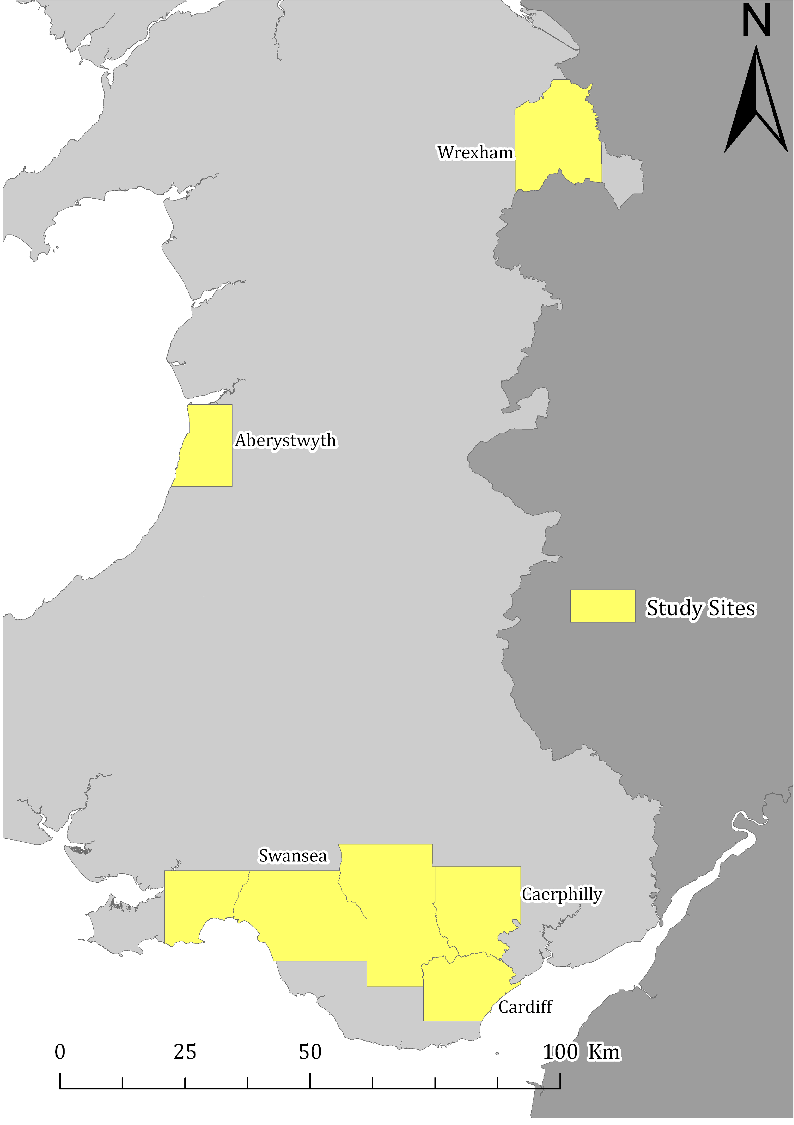
2.1. Study Sites
2.2. Datasets

| Sensor | Path | Row | Date |
|---|---|---|---|
| Landsat-5 TM | 204 | 23 | 10 February 1989 |
| Landsat-5 TM | 204 | 23 | 28 April 1989 |
| Landsat-5 TM | 204 | 24 | 28 April 1989 |
| Landsat-7 ETM+ | 204 | 23 | 24 July 1999 |
| Landsat-7 ETM+ | 204 | 24 | 24 July 1999 |
| Landsat-7 ETM+ | 204 | 23 | 10 September 1999 |
| Landsat-7 ETM+ | 204 | 24 | 10 September 1999 |
| Landsat-7 ETM+ | 204 | 23 | 13 March 2003 |
| Landsat-7 ETM+ | 204 | 24 | 13 March 2003 |
| Landsat-7 ETM+ | 203 | 23 | 22 March 2003 |
| Landsat-7 ETM+ | 203 | 24 | 22 March 2003 |
| Landsat-5 TM | 204 | 23 | 28 April 2011 |
| Landsat-5 TM | 204 | 24 | 28 April 2011 |
3. Methodology
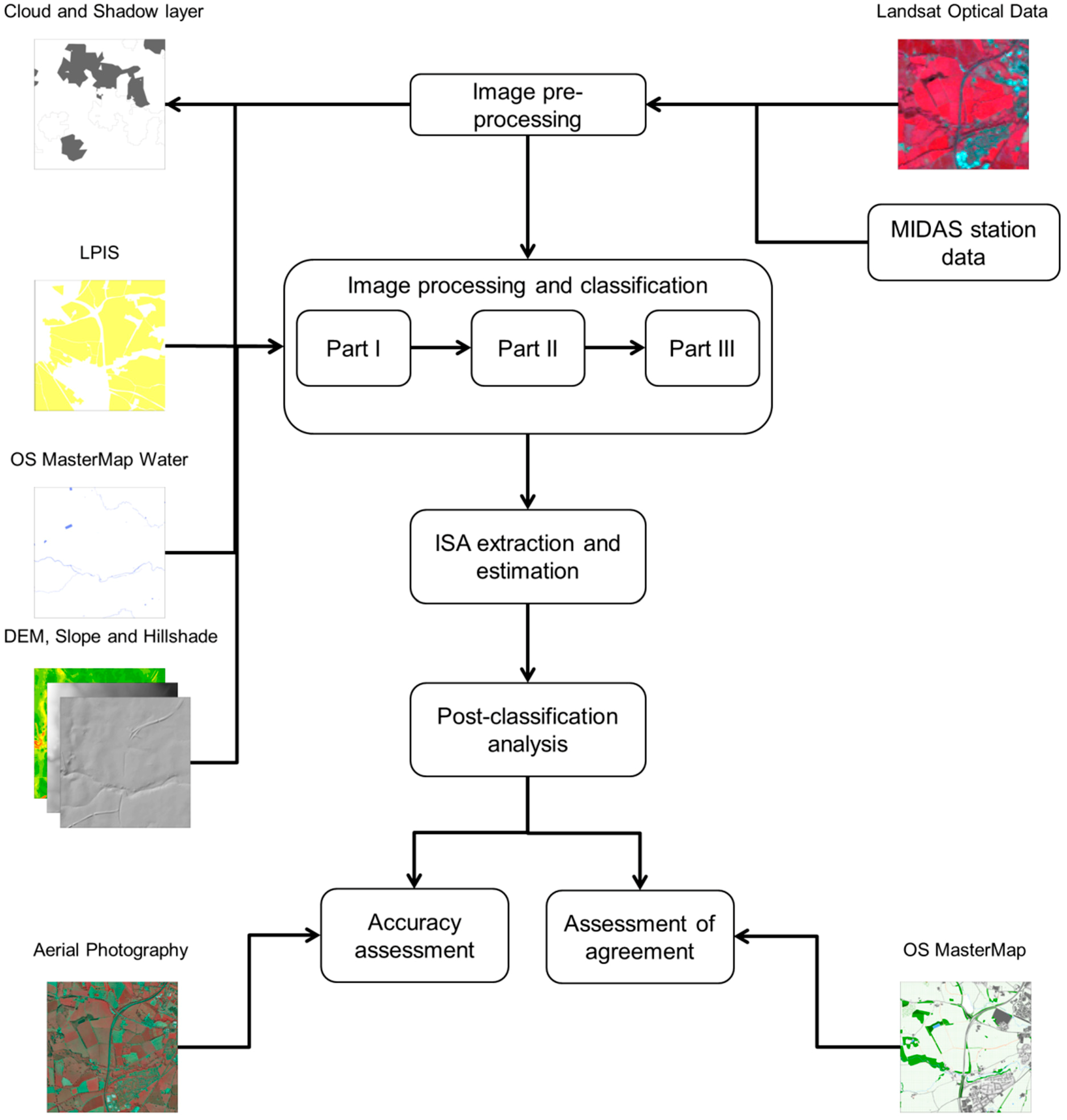
3.1. Data Pre-Processing
3.2. ISA Extraction
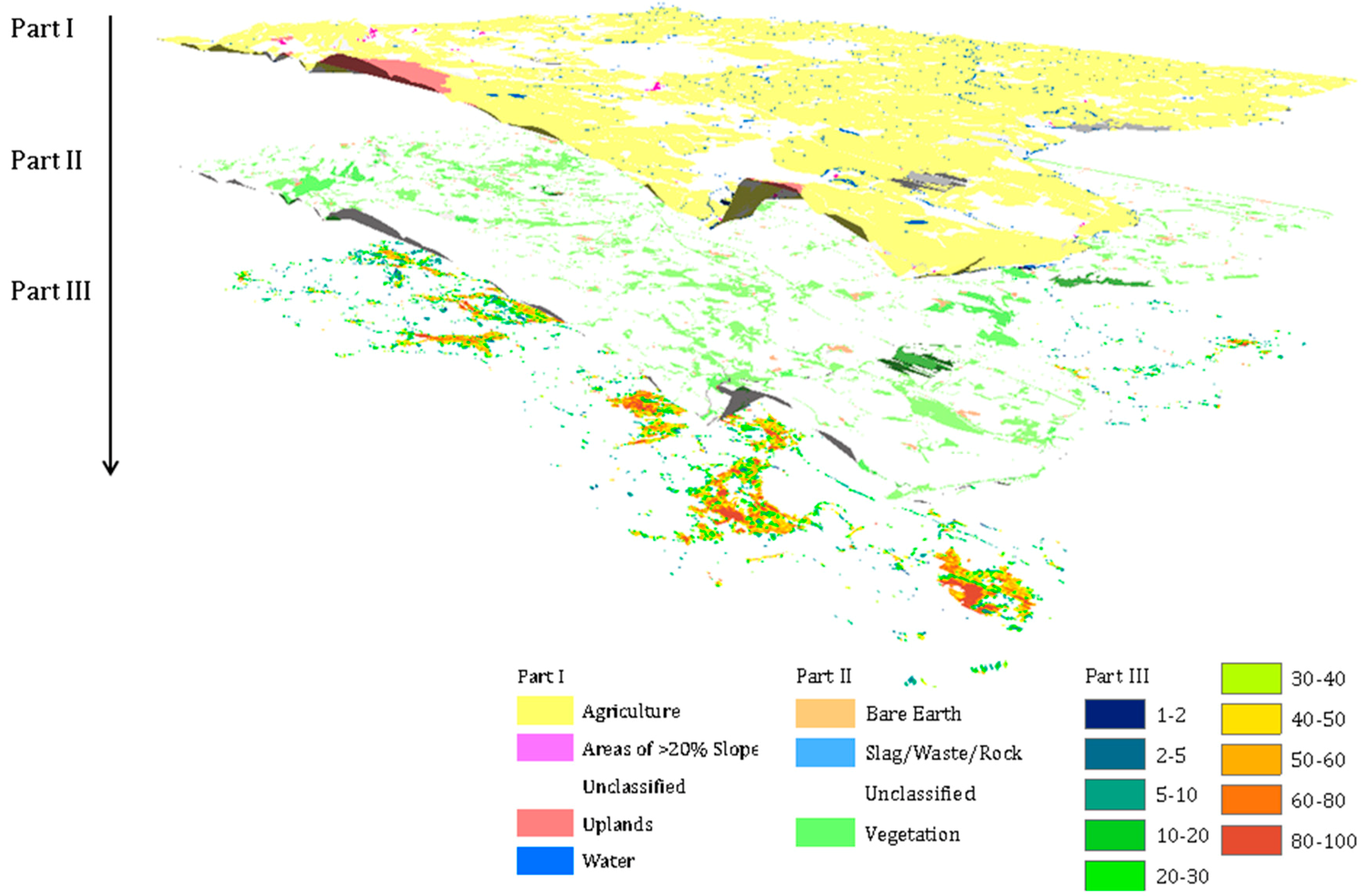
- ➢
- Spectral thresholding for the primary data in summer seasons
- ➢
- Spectral thresholding for the alternative data in other seasons
3.3. Validation
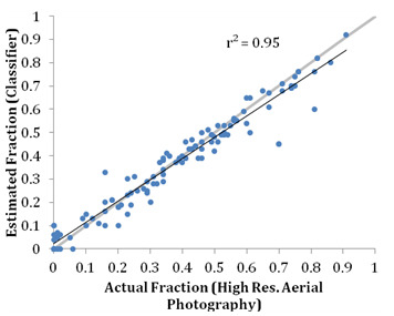
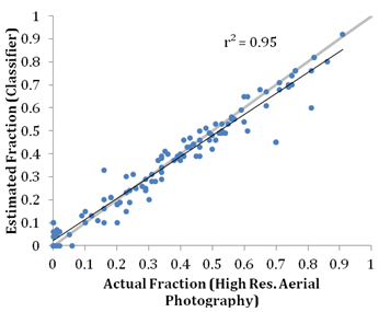
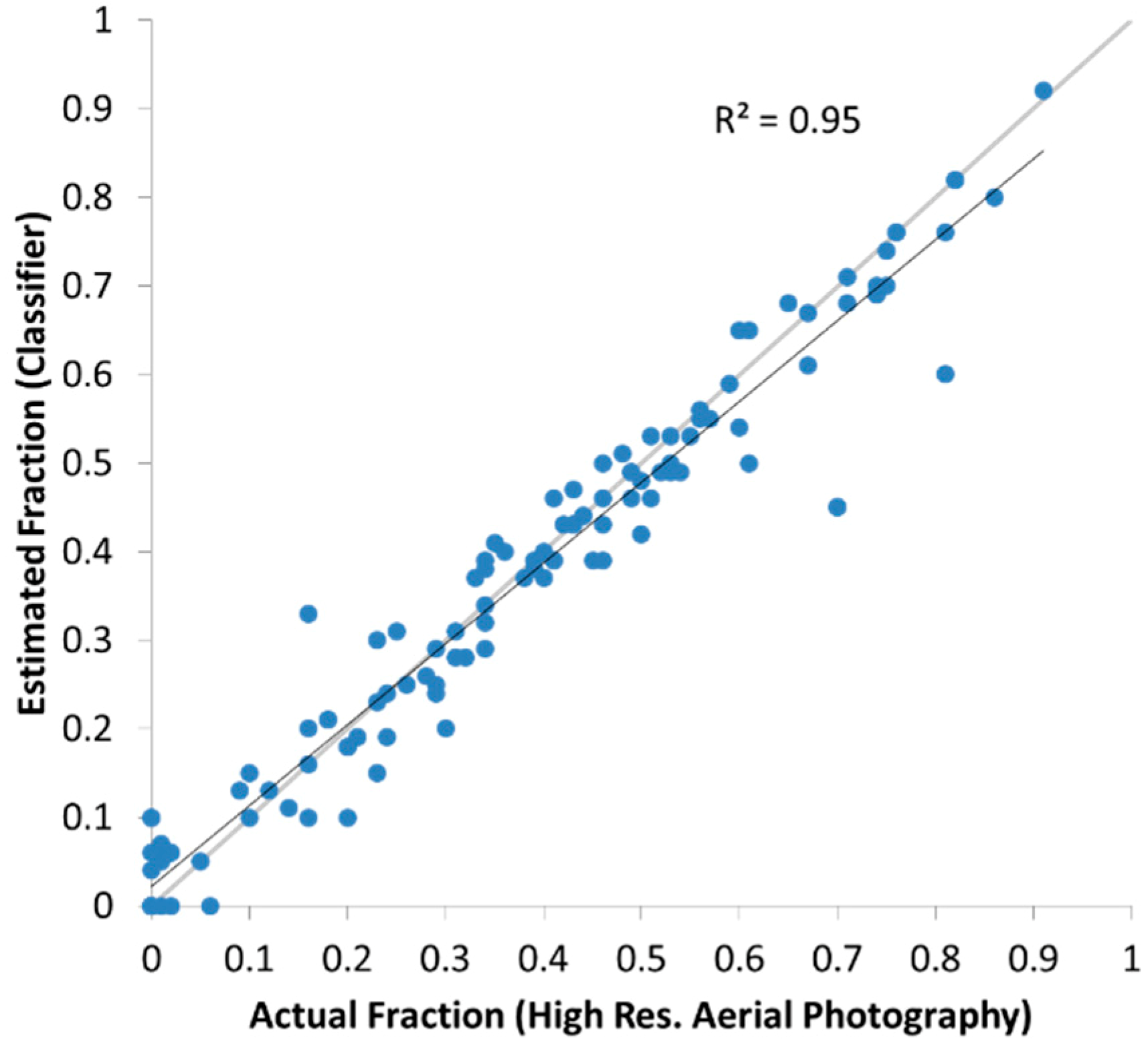
3.3.1. Accuracy Assessment
3.3.2. Assessment of Agreement
4. Results


| Study Site | DAE | SAR | FAR |
|---|---|---|---|
| Wrexham | 21.67 | 78.33 | 62.49 |
| Aberystwyth | 58.10 | 41.90 | 66.42 |
| Swansea | 86.12 | 13.88 | 59.26 |
| Neath Port Talbot | 78.61 | 21.39 | 63.69 |
| Rhondda | 77.08 | 22.92 | 60.23 |
| Caerphilly | 72.65 | 27.35 | 61.59 |
| Cardiff | 46.64 | 53.36 | 54.75 |
| Average | 62.98 | 37.02 | 61.20 |
5. Discussion
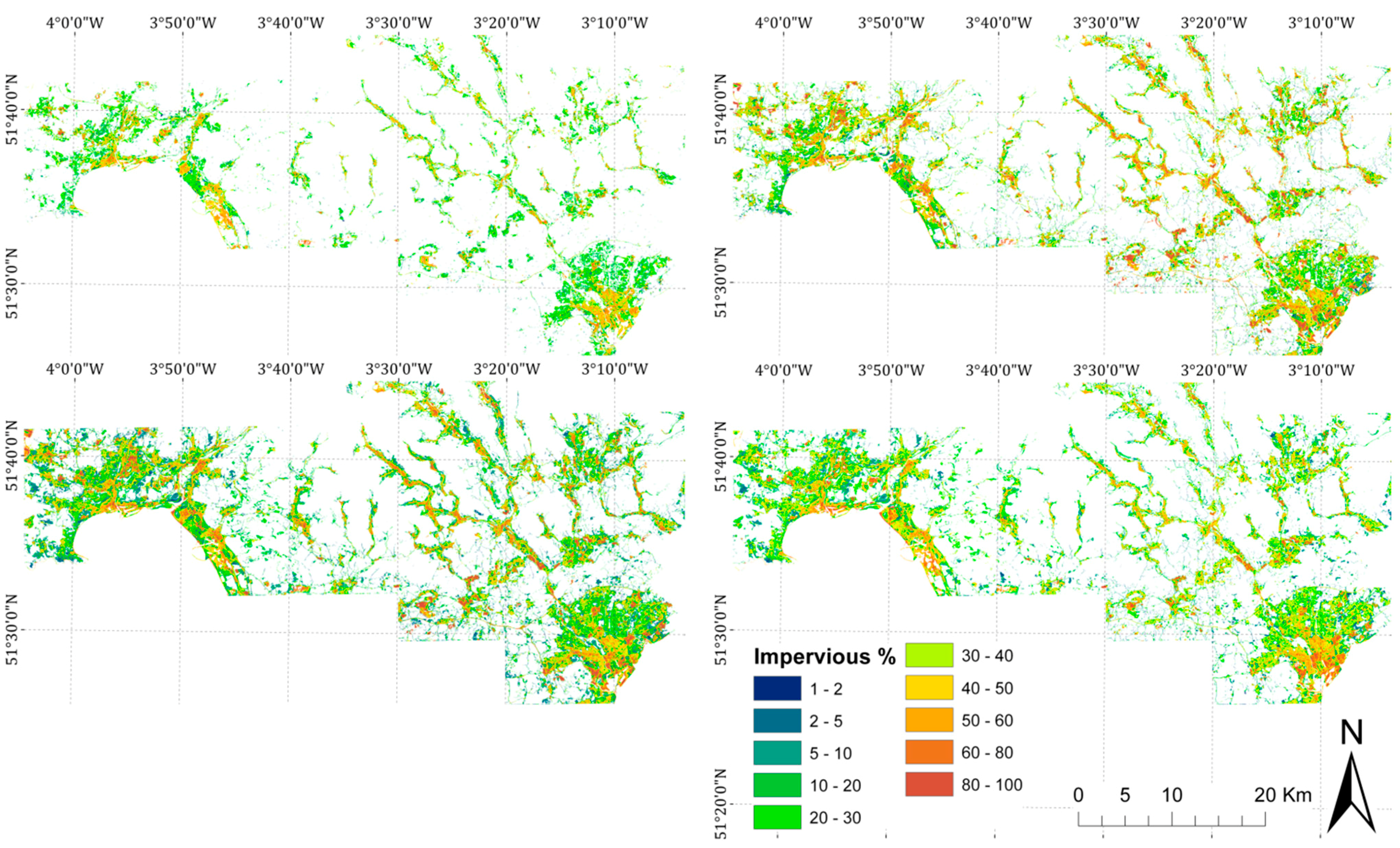
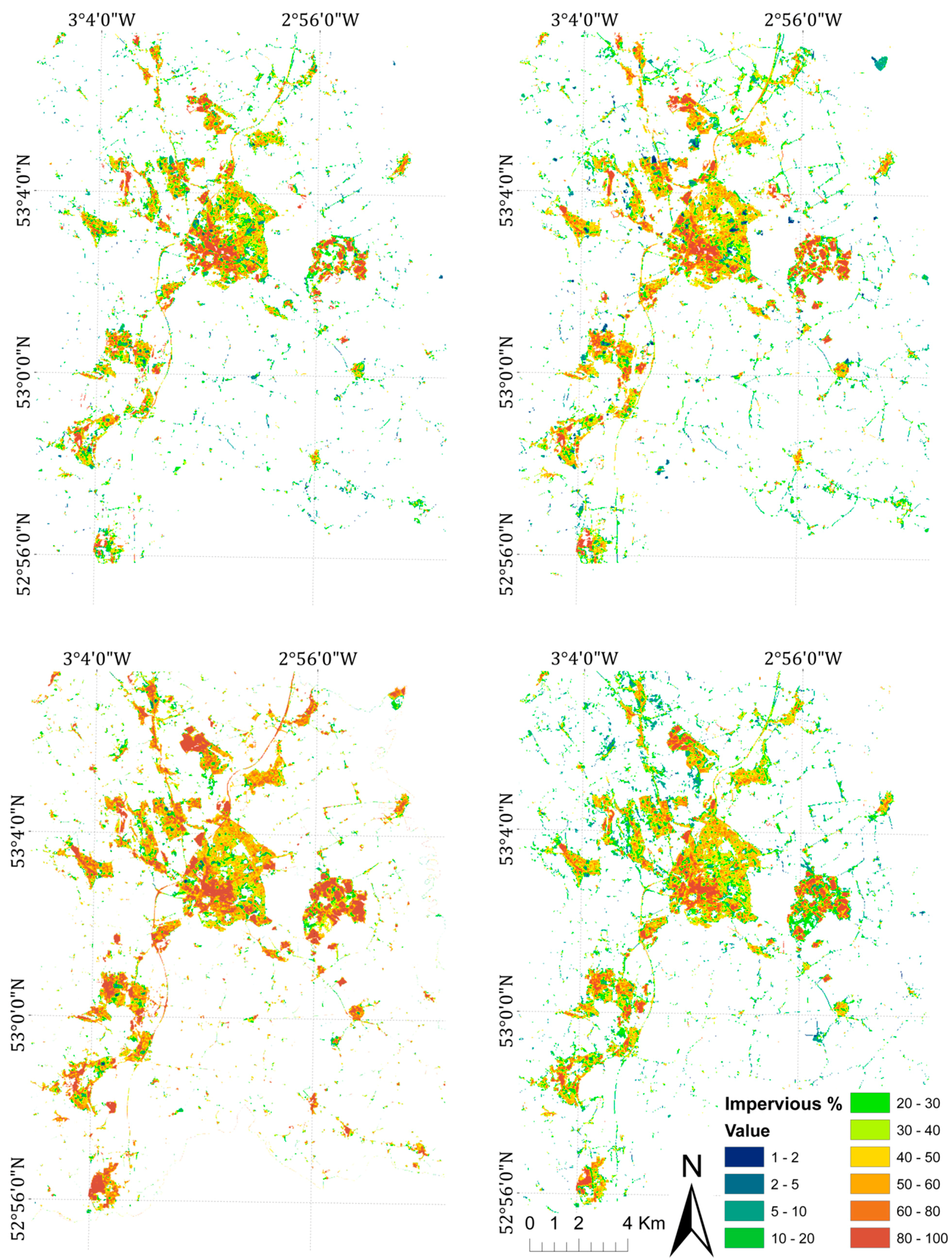
5.1. Analysis of Dynamic Changes in ISA
5.2. Comparisons with OS MM
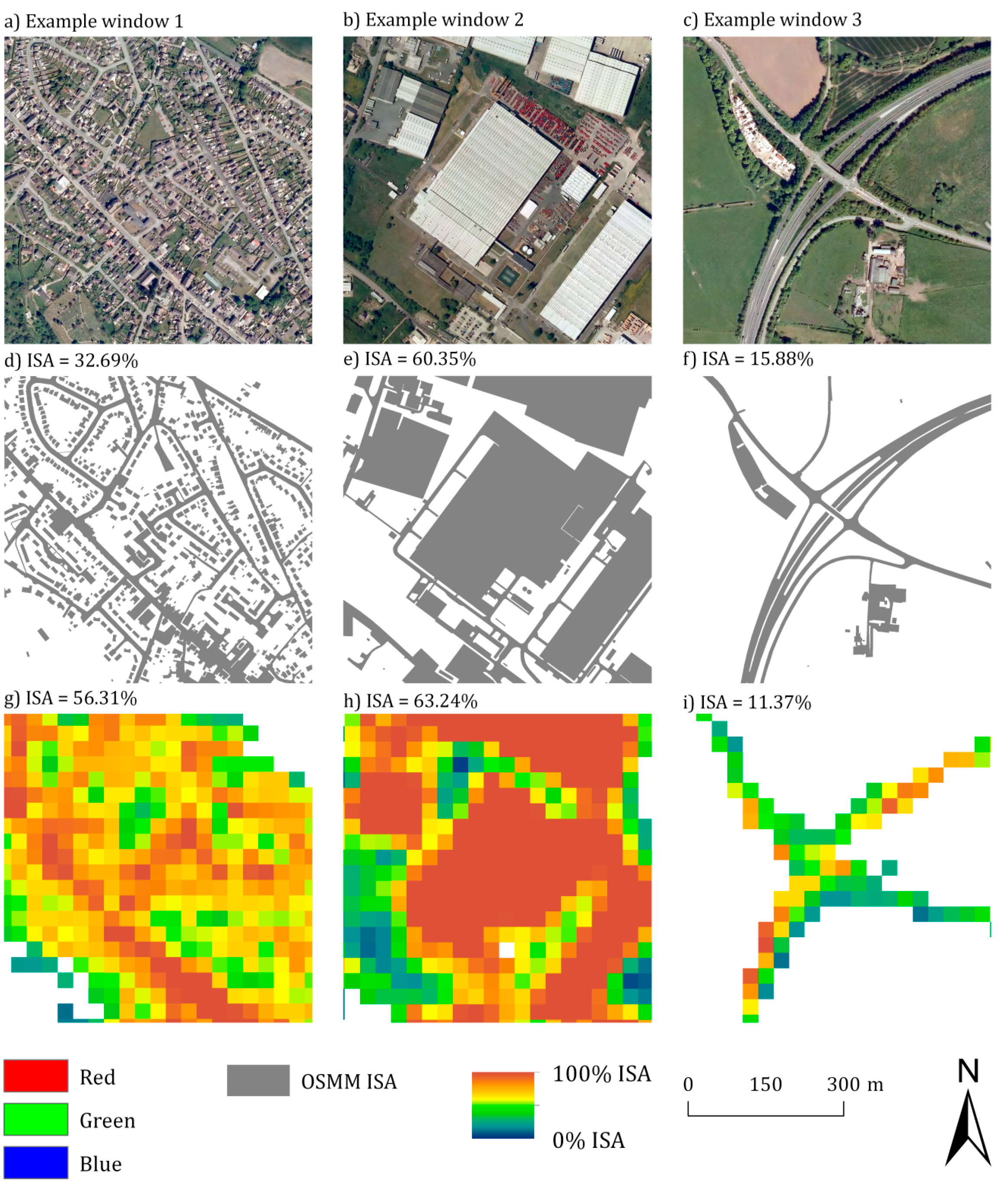
| Example Window (Figure 7) | Classifier | OSMM | AP |
|---|---|---|---|
| 1 | 56.31 | 32.69 | 50.29 |
| 2 | 63.24 | 60.35 | 62.84 |
| 3 | 11.37 | 15.88 | 13.61 |
5.3. Limitations and Recommendations
6. Conclusions
Acknowledgments
Author Contributions
Conflicts of Interest
References
- Kunzig, R. Population 7 billion. Natl Geogr. 2011, 219, 32–63. [Google Scholar]
- Webb, N.; Broomfield, M.; Cardenas, L.; MacCarthy, J.; Murrells, T.; Pang, Y.; Passant, N.; Thistlewaite, G.; Thomson, A. UK Greenhouse Gas Inventory,1990 to 2011: Annual Report for Submission under the Framework Convention on Climate Change; Ricardo-AEA: Didcot, Oxfordshire, UK, 2013; p. 816. [Google Scholar]
- Arnold, C.L.; Gibbons, C.J. Impervious surface coverage: The emergence of a key environmental indicator. J. Am. Plan. Assoc. 1996, 62, 243–258. [Google Scholar] [CrossRef]
- Hasse, J.E.; Lathrop, R.G. Land resource impact indicators of urban sprawl. Appl. Geogr. 2003, 23, 159–175. [Google Scholar] [CrossRef]
- Lee, S.; Lathrop, R.G. Subpixel analysis of Landsat ETM+ using self-organizing map (SOM) neural networks for urban land cover characterization. IEEE Trans. Geosci. Remote Sens. 2006, 44, 1642–1654. [Google Scholar] [CrossRef]
- Yang, F.; Matsushita, B.; Yang, W.; Fukushima, T. Mapping the human footprint from satellite measurements in Japan. ISPRS J. Photogramm. Remote Sens. 2014, 88, 80–90. [Google Scholar] [CrossRef] [Green Version]
- Seto, K.C.; Güneralp, B.; Hutyra, L.R. Global forecasts of urban expansion to 2030 and direct impacts on biodiversity and carbon pools. PNAS 2012, 109, 16083–16088. [Google Scholar] [CrossRef] [PubMed]
- Blaschke, T. Object based image analysis for remote sensing. ISPRS J. Photogramm. Remote Sens. 2010, 65, 2–10. [Google Scholar] [CrossRef]
- Blaschke, T.; Strobl, J. What’s wrong with pixels? Some recent developments interfacing remote sensing and GIS. GeoBIT/GIS 2001, 6, 12–17. [Google Scholar]
- Borak, J. S.; Strahler, A.H. Feature selection and land cover classification of a MODIS-like data set for a semiarid environment. Int. J. Remote Sens. 1999, 20, 919–938. [Google Scholar] [CrossRef]
- Mathur, A.; Foody, G.M. Crop classification by support vector machine with intelligently selected training data for an operational application. Int. J. Remote Sens. 2008, 29, 2227–2240. [Google Scholar] [CrossRef]
- Petropoulos, G.P.; Partsinevelos, P.; Mitraka, Z. Change detection of surface mining activity and reclamation based on a machine learning approach of multi-temporal Landsat TM imagery. Geocarto Int. 2013, 28, 323–342. [Google Scholar] [CrossRef]
- Weng, Q. Remote Sensing of Impervious Surfaces; CRC Press: Boca Raton, FL, USA, 2010. [Google Scholar]
- Frauman, E.; Wolff, E. Segmentation of very high spatial resolution satellite images in urban areas for segments-based classification. In Proceedings for 3rd International Symposium Remote Sensing and Data Fusion Over Urban Areas, Tempe, AZ, USA, 14–16 March 2005.
- Shackleford, A.K.; Davis, C.H. A combined fuzzy pixel-based and object-based approach for classification of high-resolution multispectral data over urban areas. IEEE Trans. Geosci. Remote Sens. 2003, 41, 2354–2363. [Google Scholar] [CrossRef]
- Yuan, F.; Bauer, M.E. Mapping impervious surface area using high resolution imagery: A comparison of object-based and per pixel classification. In Proceedings of ASPRS 2006 Annual Conference, Reno, NV, USA, 1–5 May 2006.
- Petropoulos, G.P.; Vadrevu, K.P.; Kalaitzidis, C. Spectral angle mapper and object-based classification combined with hyperspectral remote sensing imagery for obtaining land use/cover mapping in a Mediterranean region. Geocarto Int. 2013, 28, 114–129. [Google Scholar] [CrossRef]
- Petropoulos, G. P.; Kalaitzidis, C.; Prasad Vadrevu, K. Support vector machines and object-based classification for obtaining land-use/cover cartography from Hyperion hyperspectral imagery. Comput. Geosci. 2012, 41, 99–107. [Google Scholar] [CrossRef]
- Weng, Q. Remote sensing of impervious surfaces in the urban areas: Requirements, methods, and trends. Remote Sens. Environ. 2012, 117, 34–49. [Google Scholar] [CrossRef]
- Ling, F.; Li, X.; Xiao, F.; Fang, S.; Du, Y. Object-based sub-pixel mapping of buildings incorporating the prior shape information from remotely sensed imagery. Int. J. Appl. Earth Obs. Geoinf. 2012, 18, 283–292. [Google Scholar] [CrossRef]
- Fankhauser, R. Automatic determination of imperviousness in urban areas from digital orthophotos. Water Sci. Technol. 1999, 39, 81–86. [Google Scholar] [CrossRef]
- Weng, Q. Modelling urban growth effects on surface runoff with the integration of remote sensing and GIS. Environ. Manag. 2001, 28, 737–748. [Google Scholar] [CrossRef]
- Dams, J.; Dujardin, J.; Reggers, R.; Bashir, I.; Canters, F.; Batelaan, O. Mapping impervious surface change from remote sensing for hydrological modelling. J. Hydrol. 2013, 485, 84–95. [Google Scholar] [CrossRef]
- Berezowski, T.; Chormanski, J.; Batelaan, O.; Canters, F.; Van de Vorde, T. Quantifying land-cover proportions for urban runoff prediction. The advantage of distributed remote sensing techniques. In Proceedings of EGU General Assembly 2012, Vienna, Austria, 22–27 April 2012.
- Hu, X.; Weng, Q. Estimating impervious surfaces from medium spatial resolution imagery: A comparison between fuzzy classification and LSMA. Int. J. Remote Sens. 2011, 32, 5645–5663. [Google Scholar] [CrossRef]
- Weng, Q.; Rajasekar, U.; Hu, X. Modelling urban heat islands and their relationship with impervious surface and vegetation abundance by using ASTER images. IEEE Trans. Geosci. Remote Sens. 2011, 49, 4080–4089. [Google Scholar] [CrossRef]
- Liu, H.; Weng, Q. Landscape metrics for analysing urbanization-induced land use and land cover changes. Geocarto Int. 2013, 28, 582–593. [Google Scholar] [CrossRef]
- Quarmby, N.A.; Cushine, J.L. Monitoring urban land cover changes at the urban fringe from SPOT HRV imagery in south-east England. Int. J. Remote Sens. 1989, 10, 953–963. [Google Scholar] [CrossRef]
- Fuller, R.M.; Groom, G.B.; Jones, A.R. The land cover map of Great Britain: An automated classification of Landsat Thematic Mapper data. Photogramm. Eng. Remote Sens. 1994, 60, 553–562. [Google Scholar]
- Grey, W.M.F.; Luckman, A.J.; Holland, D. Mapping urban change in the UK using satellite radar interferometry. Remote Sens. Environ. 2003, 87, 16–22. [Google Scholar] [CrossRef]
- Kampouraki, M.; Wood, G.A.; Brewer, T. The application of remote sensing to identify and measure sealed areas in urban environments. In Proceeding from ISPRS 1st International Conference on Object-Based Image Analysis (OBIS 2006), Salzburg, Austria, 4–5 July 2006.
- Martinuzzi, S.; Gould, W.A.; González, O.M.R. Creating Cloud-Free Landsat ETM+ Data Sets in Tropical Landscapes: Cloud and Cloud-Shadow Removal; IITF-GTR-32; U.S. Department of Agriculture, Forest Service, International Institute of Tropical Forestry: Portland, OR, USA, 2007. [Google Scholar]
- Gurney, C.M. The use of contextual information to detect cumulous clouds and cloud shadow in Landsat data. Int. J. Remote Sens. 1982, 3, 51–62. [Google Scholar] [CrossRef]
- Irish, R. Landsat 7 automatic cloud cover assessment. Proc. SPIE 2000, 4049, 348–355. [Google Scholar]
- Irish, R.; Barker, J.; Goward, S.; Arvidson, T. Characterization of the Landsat-7 ETM+ automated cloud-cover assessment (ACCA) algorithm. Photogramm. Eng. Remote Sens. 2006, 72, 1179–1188. [Google Scholar] [CrossRef]
- Wang, B.; Ono, A.; Muramatsu, K.; Fujiwara, N. Automated detection and removal of clouds and their shadows from Landsat TM images. IEICE Trans. Inf. Syst. 1999, E82-D, 453–460. [Google Scholar]
- Zhu, Z.; Woodcock, C.E. Object-based cloud and cloud shadow detection in Landsat imagery. Remote Sens. Environ. 2012, 118, 83–94. [Google Scholar] [CrossRef]
- Jin, S.; Homer, C.; Yang, L.; Xian, G.; Fry, J.; Danielson, P.; Townsend, P.A. Automated cloud and shadow detection and filling using two-date Landsat imagery in the USA. Int. J. Remote Sens. 2012, 34, 1540–1560. [Google Scholar] [CrossRef]
- Goodwin, N.R.; Collett, L.J.; Denham, R.J.; Flood, N.; Tindall, D. Cloud and cloud shadow screening across Queensland Australia: An automated method for Landsat TM/ETM+ time series. Remote Sens. Environ. 2013, 134, 50–65. [Google Scholar] [CrossRef]
- Li, D.; Tang, P. A sensor specified method based on spectral transformation for masking cloud in Landsat data. IEEE J. Sel. Top. Appl. Earth Obs. Remote Sens. 2013, 6, 1619–1627. [Google Scholar] [CrossRef]
- Small, C. Estimation of urban vegetation abundance by spectral mixture analysis. Int. J. Remote Sens. 2001, 22, 1305–1334. [Google Scholar] [CrossRef]
- Phinn, S.; Stanford, M.; Scarth, P.; Murray, A.T.; Shyy, P.T. Monitoring the composition of urban environments based on the vegetation-impervious surface-soil (VIS) model by subpixel analysis techniques. Int. J. Remote Sens. 2002, 23, 4131–4153. [Google Scholar] [CrossRef]
- Wu, C.; Murray, A.T. Estimating impervious surface distribution by spectral mixture analysis. Remote Sens. Environ. 2003, 84, 493–505. [Google Scholar] [CrossRef]
- Song, C. Spectral mixture analysis for subpixel vegetation fractions in the urban environment: How to incorporate endmember variability? Remote Sens. Environ. 2005, 95, 248–263. [Google Scholar] [CrossRef]
- Lu, D.; Weng, Q. Use of impervious surface in urban land-use classification. Remote Sens. Environ. 2006, 102, 146–160. [Google Scholar] [CrossRef]
- Lu, D.; Moran, E.; Hetrick, S. Detection of impervious surface change with multitemporal Landsat images in an urban-rural frontier. ISPRS J. Photogramm. Remote Sens. 2011, 66, 298–306. [Google Scholar] [CrossRef] [PubMed]
- Lu, D.; Li, G.; Moran, E.; Batistella, M.; Freitas, C. Mapping impervious surfaces with the integrated use of Landsat Thematic Mapper and radar data: A case study in an urban-rural landscape in the Brazillian Amazon. ISPRS J. Photogramm. Remote Sens. 2011, 66, 798–808. [Google Scholar] [CrossRef] [Green Version]
- Ridd, M.K. Exploring a VIS (vegetation-impervious surface-soil) model for urban ecosystem analysis through remote sensing: Comparative anatomy for cities. Int. J. Remote Sens. 1995, 16, 2165–2185. [Google Scholar] [CrossRef]
- Hu, X.; Weng, Q. Estimating impervious surfaces from medium spatial resolution imagery using the self-organizing map and multi-layer perception neural networks. Remote Sens. Environ. 2009, 113, 2089–2102. [Google Scholar] [CrossRef]
- Lee, S.; Lathrop, R.G. Sub-pixel estimation of urban land cover components with linear mixture model analysis and Landsat Thematic Mapper imagery. Int. J. Remote Sens. 2005, 26, 4885–4905. [Google Scholar] [CrossRef]
- Jones, P.S.; Stevens, D.P.; Blackstock, T.H.; Burrows, C.R.; Howe, E.A. Priority Habitats of Wales: A Technical Guide; Countryside Council for Wales: Bangor, UK, 2003. [Google Scholar]
- Joint Nature Conservation Committee. Handbook for Phase 1 Habitat Survey—A Technique for Environmental Audit; Joint Nature Conservation Committee: Peterborough, UK, 2010. [Google Scholar]
- Revell, P.; Regnauls, N.; Thom, S. Generalising OS MasterMap® topographic buildings and ITN road centerlines to 1:50000 scale using a spatial hierarchy of agents, triangulation and topology. In Proceedings of the International Cartographic Conference, A Coruna, Spain, 9–16 July 2005.
- Smith, G.B.; Boyd, M.; Downs, M.; Gregory, T.; Morton, M.; Brown, D.; Thomson, N.A. UK land cover map production through the generalisation of OS MasterMap®. Cartogr. J. 2007, 44, 276–283. [Google Scholar] [CrossRef]
- Thomson, M.K. Dwelling on Ontology-Semantic Reasoning over Topographic Maps. Ph.D. Thesis, University College London, London, UK, 2009. [Google Scholar]
- Kuntz, S.; Schmeer, E.; Jochum, M.; Smith, G. Towards an European land cover monitoring service and high-resolution layers. In Land Use and Land Cover Mapping in Europe; Manakos, I., Braun, M., Eds.; Springer: Dordrecht, The Netherlands, 2014; pp. 43–52. [Google Scholar]
- Lefebvre, A.; Beaugendre, N.; Pennec, A.; Sannier, C.; Corpetti, T. Using data fusion to update built-up areas of the 2012 European High-Resolution Layer Imperviousness. In Proceedings of the 33rd EARSeL Symposium Conference, Matera, Italy, 3–6 June 2013; pp. 321–328.
- Lucas, R.; Medcalf, K.; Brown, A.; Bunting, P.; Breyer, J.; Clewley, D.; Keyworth, S.; Blackmore, P. Updating the Phase 1 habitat map of Wales, UK, using satellite sensor data. ISPRS J. Photogramm. Remote Sens. 2011, 66, 81–102. [Google Scholar] [CrossRef]
- Baxter, R.; Lees, L. The rebirth of high-rise living in London: Towards a sustainable, inclusive, and liveable urban form. In Regenerating London: Governance, Sustainability and Community in a Global City; Routledge: London, UK, 2009; pp. 151–172. [Google Scholar]
- Teh, H.T.; Lim, H.S.; Matjafri, M.Z. Deriving urban sealed surface density map using linear spectral unmixing analysis. In Proceedings of 2011 IEEE International Conference on Space Science and Communication (IconSpace), Penang, Malaysia, 12–13 July 2011.
- Zhu, S.; Zhang, G. Analysis on relationship between urban land surface temperature and landcover from Landsat ETM+ data. In Proceedings of 2011 Fourth International Symposium on Knowledge Acquisition and Modeling (KAM), Sanya, China, 8–9 October 2011.
- Sagris, V.; Devos, W. LPIS Core Conceptual Model: Methodology for Feature Catalogue and Application Schema; Joint Research Centre: Ispra, Italy, 2008. [Google Scholar]
- Deng, C.; Wu, C. BCI: A biophysical composition index for remote sensing of urban environments. Remote Sens. Environ. 2012, 127, 247–259. [Google Scholar] [CrossRef]
- Settle, J.J.; Drake, N.A. Linear mixing and the estimation of ground cover proportions. Int. J. Remote Sens. 1993, 14, 1159–1177. [Google Scholar] [CrossRef]
- Kauth, R.J.; Thomas, G.S. The tasselled cap—A graphic description of the spectral-temporal development of agricultural crops as seen by Landsat. In Proceedings of the Symposium on Machine Processing of Remotely Sensed Data, West Lafayette, IN, USA, 29 June–1 July 1976.
- Huang, C.; Wylie, B.; Yang, L.; Homer, C.; Zylstra, G. Derivation of a tasselled cap transformation based on Landsat 7 at-satellite reflectance. Int. J. Remote Sens. 2002, 23, 1741–1748. [Google Scholar] [CrossRef]
- Congalton, R.G. A review of assessing the accuracy of classifications of remotely sensed data. Remote Sens. Environ. 1991, 37, 35–46. [Google Scholar] [CrossRef]
- Congalton, R.G.; Green, K. Assessing the Accuracy of Remotely Sensed Data: Principles and Practices, 2nd ed.; CRC Press: Boca Raton, FL, USA, 2008. [Google Scholar]
- Foody, G.M. Status of land cover classification accuracy assessment. Remote Sens. Environ. 2002, 80, 185–201. [Google Scholar] [CrossRef]
- Bauer, M.E.; Loffelholz, B.C.; Wilson, B. Estimating and mapping impervious surface area by regression analysis of Landsat imagery. In Remote Sensing of Impervious Surfaces; Weng, Q., Ed.; Taylor & Francis Group: Boca Raton, FL, USA, 2008; pp. 31–47. [Google Scholar]
- Wu, C. Normalized spectral mixture analysis for monitoring urban composition using ETM+ imagery. Remote Sens. Enviorn. 2004, 93, 480–492. [Google Scholar] [CrossRef]
- Kontoes, C.C.; Poilve, H.; Florsch, G.; Keramitsoglou, I.; Paralikidis, S. A comparative analysis of a fixed thresholding vs. a classification tree approach for operational burn scar detection and mapping. Int. J. Appl. Earth Obs. Geoinf. 2009, 11, 299–316. [Google Scholar] [CrossRef]
- Petropoulos, G.P.; Kontoes, C.C.; Keramitsoglou, I. Land cover mapping with emphasis to burnt area delineation using co-orbital ALI and Landsat TM imagery. Int. J. Appl. Earth Obs. Geoinf. 2012, 18, 344–355. [Google Scholar] [CrossRef]
- Dallimer, M.; Tang, Z.; Bibby, P.R.; Brindley, P.; Gaston, K.J.; Davies, Z.G. Temporal changes in greenspace in a highly urbanized region. Biol. Lett. 2011, 7, 763–766. [Google Scholar] [CrossRef] [PubMed]
- Smith, G.M. Land use & land cover mapping in Europe: Examples from the UK. In Land Use and Land Cover Mapping in Europe, 1st ed.; Manakos, I., Braun, M., Eds.; Springer: Dordrecht, The Netherlands, 2014; pp. 273–282. [Google Scholar]
- Jones, J.W.; Jarnagin, T. Evaluation of a moderate resolution, satellite-based impervious surface map using an independent, high-resolution validation data set. J. Hydrol. Eng. 2009, 14, 369–376. [Google Scholar] [CrossRef]
© 2014 by the authors; licensee MDPI, Basel, Switzerland. This article is an open access article distributed under the terms and conditions of the Creative Commons Attribution license (http://creativecommons.org/licenses/by/4.0/).
Share and Cite
Scott, D.; Petropoulos, G.P.; Moxley, J.; Malcolm, H. Quantifying the Physical Composition of Urban Morphology throughout Wales Based on the Time Series (1989–2011) Analysis of Landsat TM/ETM+ Images and Supporting GIS Data. Remote Sens. 2014, 6, 11731-11752. https://doi.org/10.3390/rs61211731
Scott D, Petropoulos GP, Moxley J, Malcolm H. Quantifying the Physical Composition of Urban Morphology throughout Wales Based on the Time Series (1989–2011) Analysis of Landsat TM/ETM+ Images and Supporting GIS Data. Remote Sensing. 2014; 6(12):11731-11752. https://doi.org/10.3390/rs61211731
Chicago/Turabian StyleScott, Douglas, George P. Petropoulos, Janet Moxley, and Heath Malcolm. 2014. "Quantifying the Physical Composition of Urban Morphology throughout Wales Based on the Time Series (1989–2011) Analysis of Landsat TM/ETM+ Images and Supporting GIS Data" Remote Sensing 6, no. 12: 11731-11752. https://doi.org/10.3390/rs61211731