Identification of Ecosystem Functional Types from Coarse Resolution Imagery Using a Self-Organizing Map Approach: A Case Study for Spain

 ,
,
Abstract
:
1. Introduction
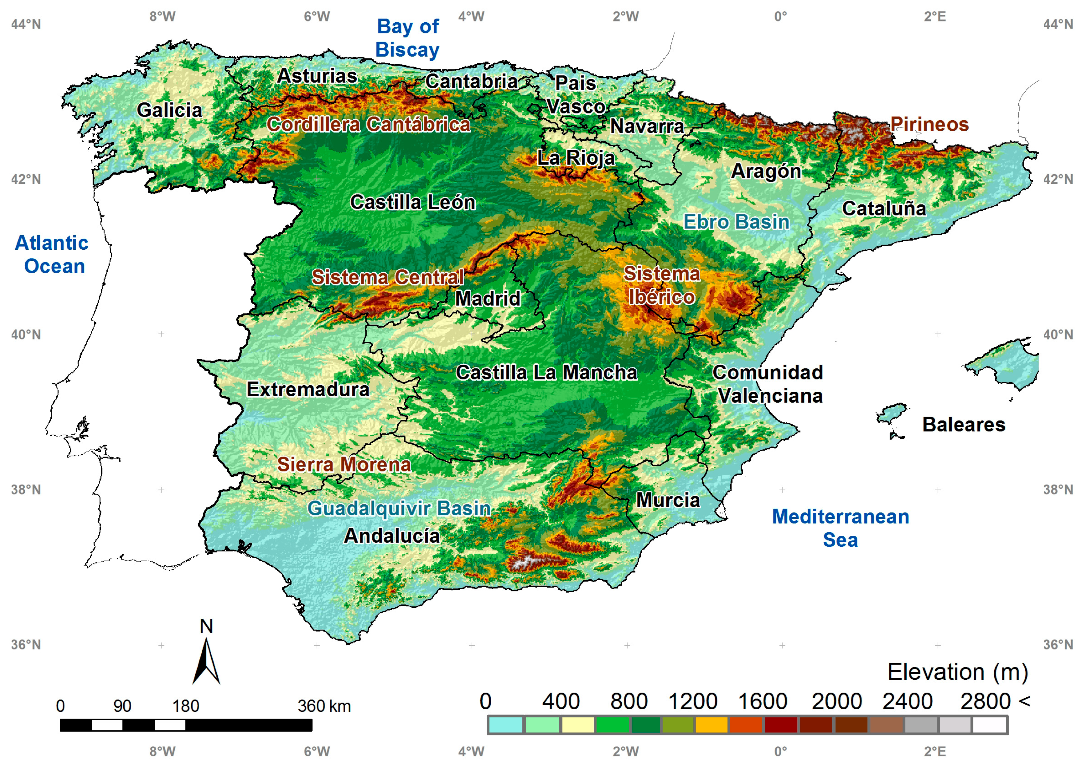
2. Study Area
3. Data Set
3.1. Normalized Difference Vegetation Index (NDVI)
3.2. Land Surface Temperature (LST)
3.3. Albedo
3.4. Precipitation Data
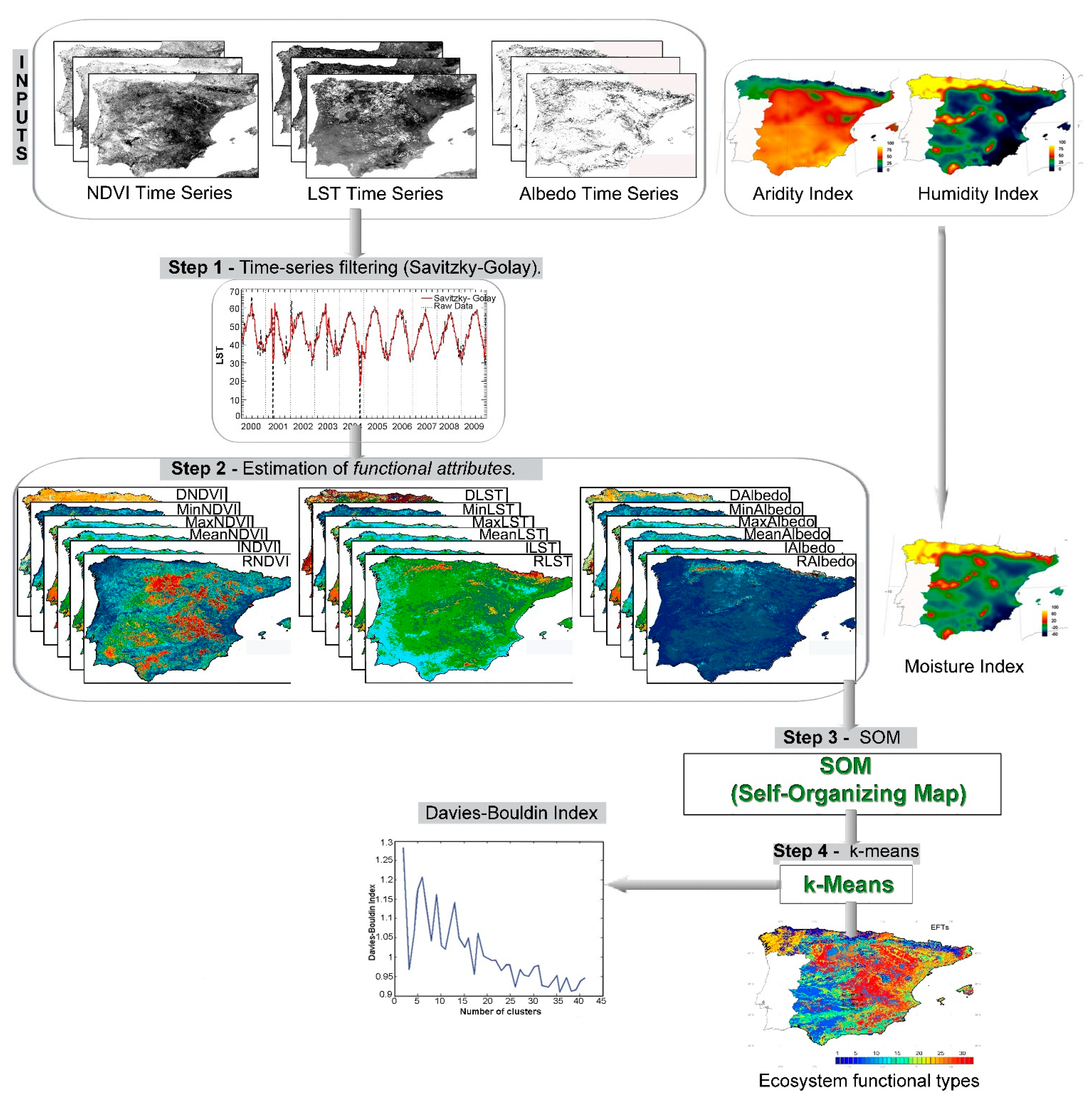
4. EFTs Classification Scheme
4.1. Time-Series Filtering

4.2. Estimation of Functional Attributes
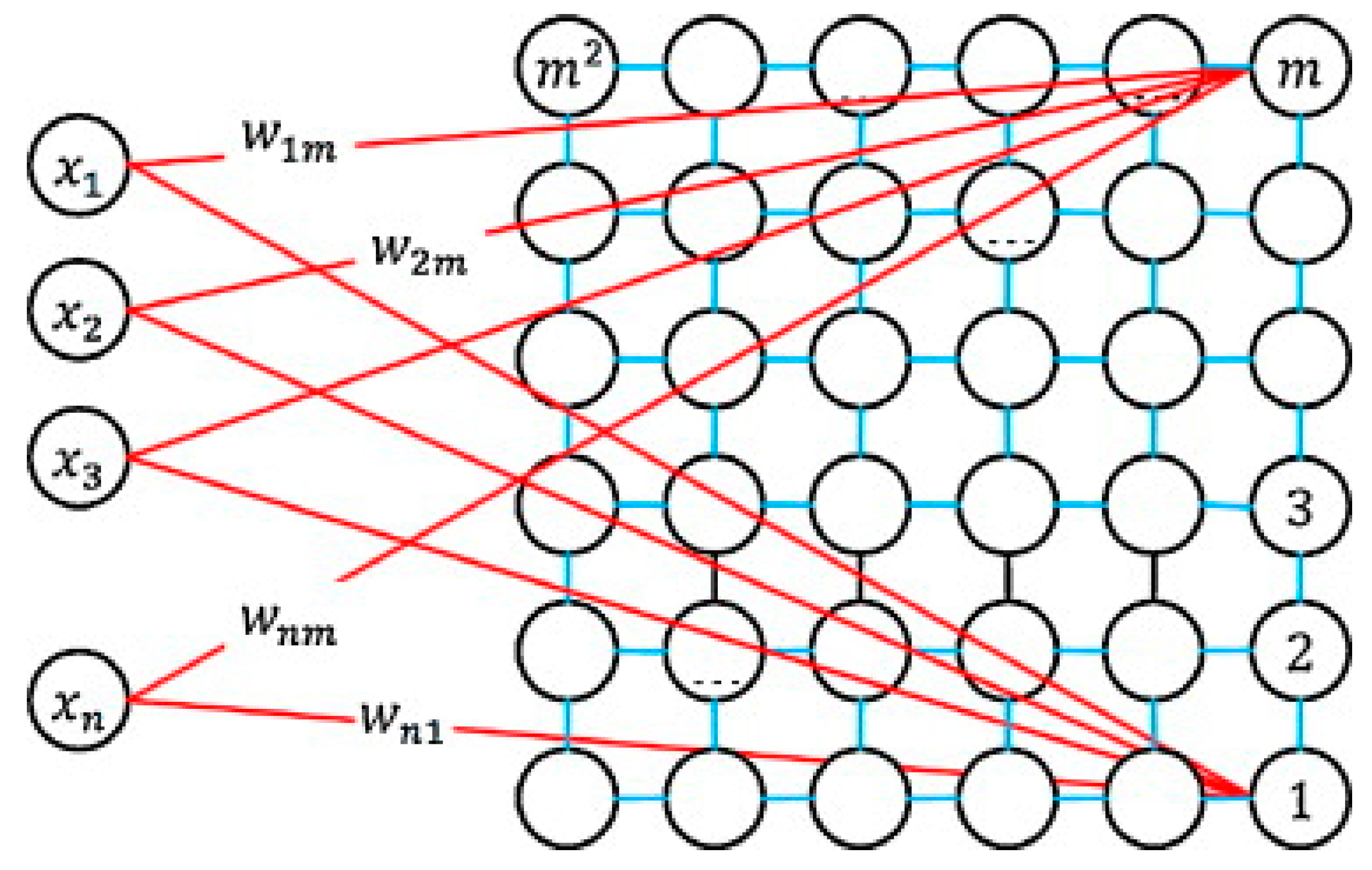
4.3. Kohonen Self-Organizing Map (SOM)

- (1)
- Initialization: the M weight vectors are initialized to a random value between 0 and 1.
- (2)
- Competition: each input vector in the training set, x, is compared with each weight vector, wj, to determine the neuron j which is the closest in terms of distance. This winning output node or neuron c(j), which is called Best-Matching Unit (BMU), is typically computed using the minimum-distance Euclidean through the following rule:
- (3)
- Cooperation: in this stage it is necessary to define a neighborhood function that allows to identify the output nodes close to the BMU, c(j), to be updated in the next step.
- (4)
- Updating: the weight vector of neurons close to the BMU, as well as the weight vector of the BMU itself, are updated according to:where t denotes time, α(t) is learning rate with an initial value between 0 and 1, hci(r(t)) denotes the neighborhood kernel around the winner unit c, with neighborhood radius r(t).
- (5)
- Repetition: Repeat steps 2 and 3 until the network convergence, where the learning rate and neighborhood decrease monotonically with time.
4.4. K-means Classification
5. Results and Discussion
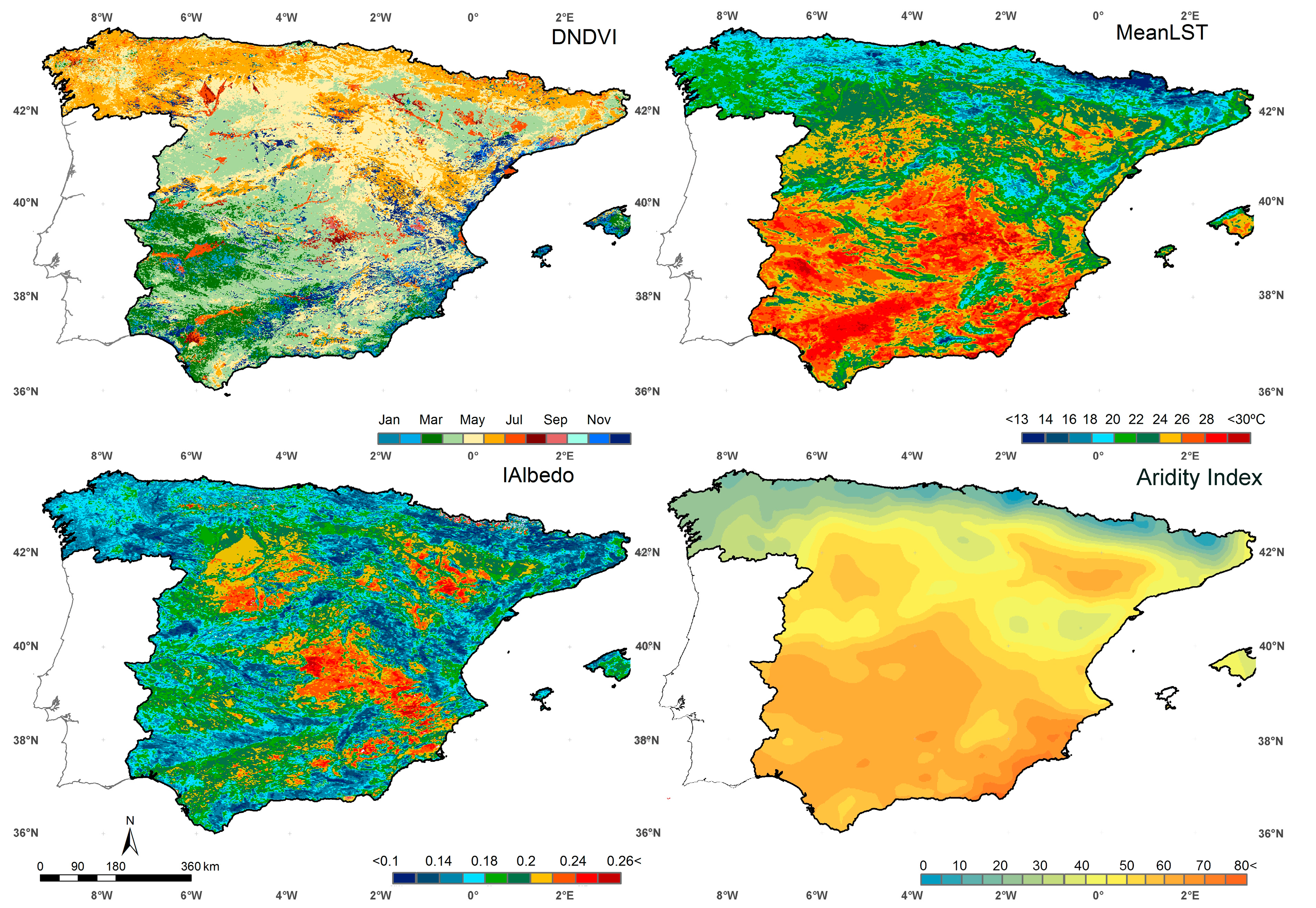
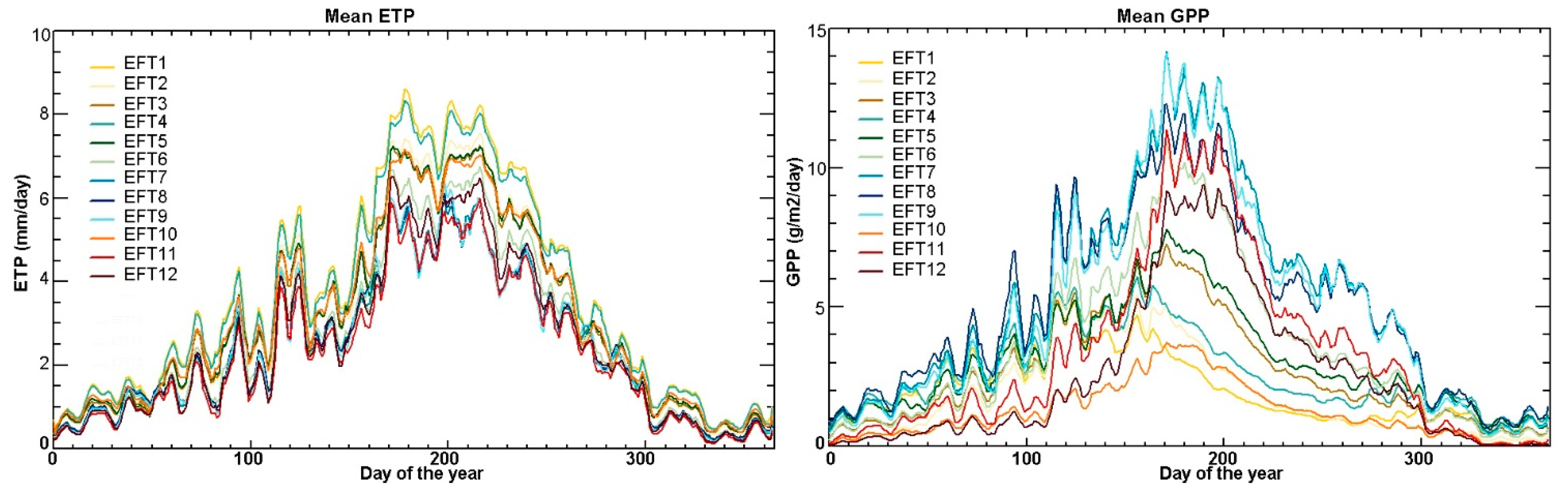
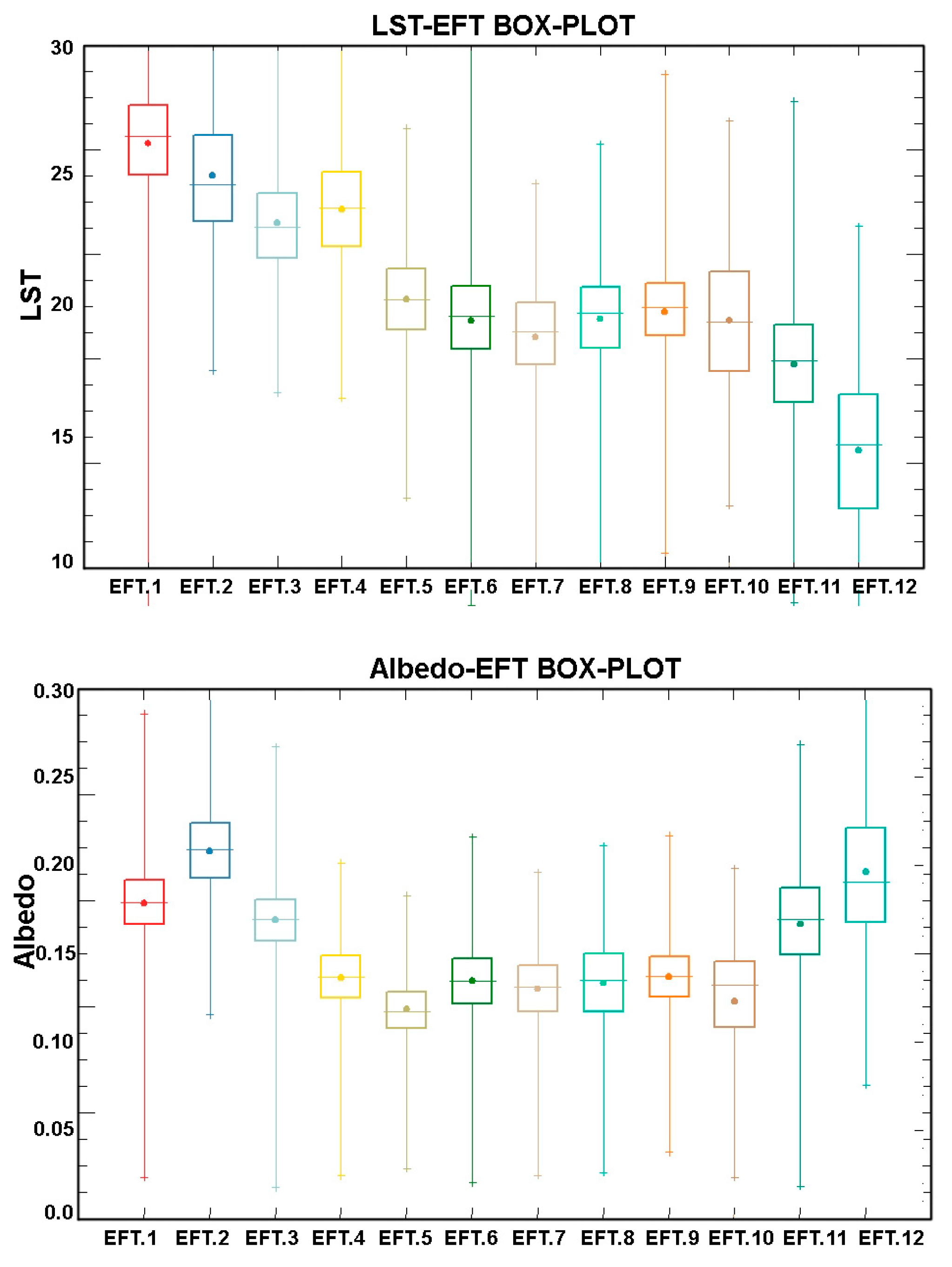
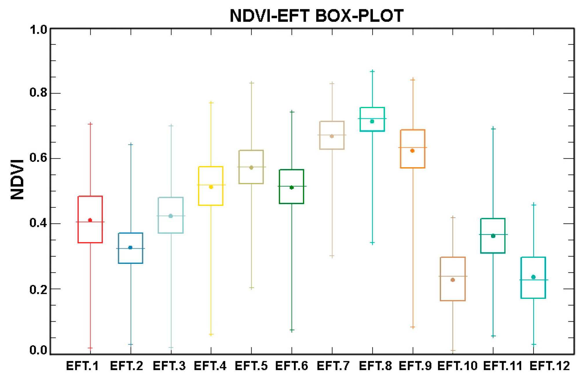
5.1. Examples of Functional Attributes

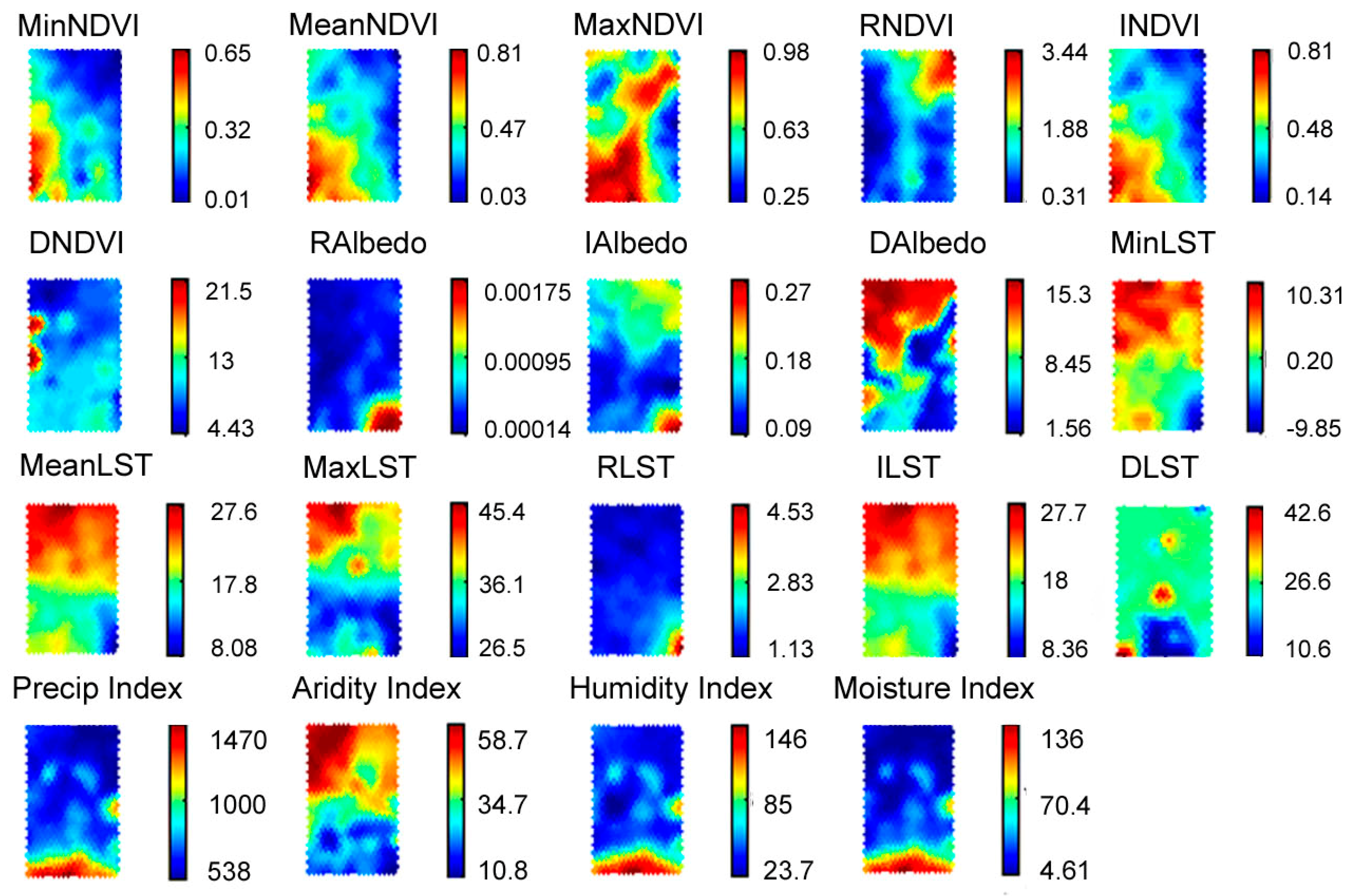
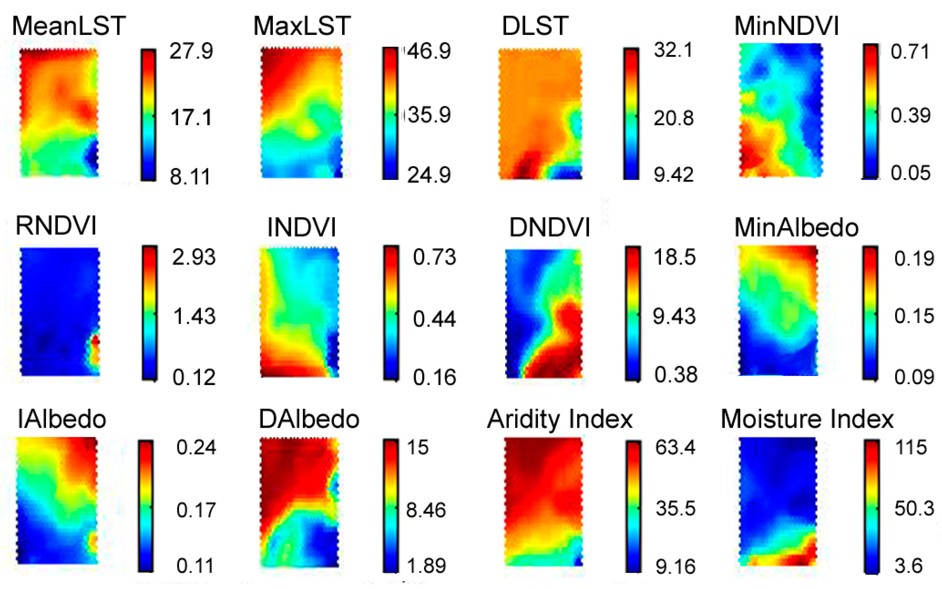
5.2. Training SOM


| Map Size | 100 | 200 | 300 | 400 | 500 | 600 | 700 | 800 | 900 |
|---|---|---|---|---|---|---|---|---|---|
| Qe | 2.08 | 1.82 | 1.67 | 1.57 | 1.44 | 1.39 | 1.35 | 1.31 | 1.30 |
| Te | 0.045 | 0.057 | 0.049 | 0.05 | 0.048 | 0.034 | 0.033 | 0.032 | 0.031 |
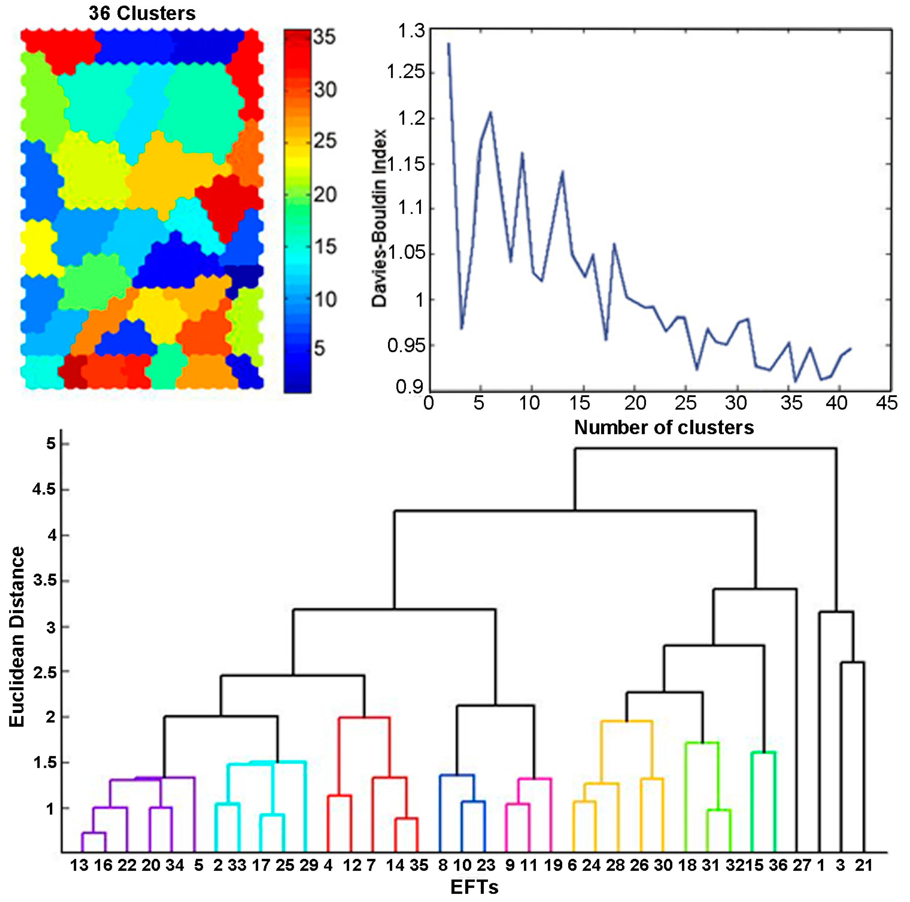
5.3. Clustering of the SOM

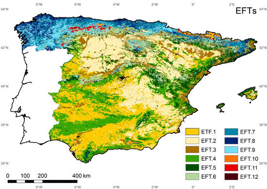
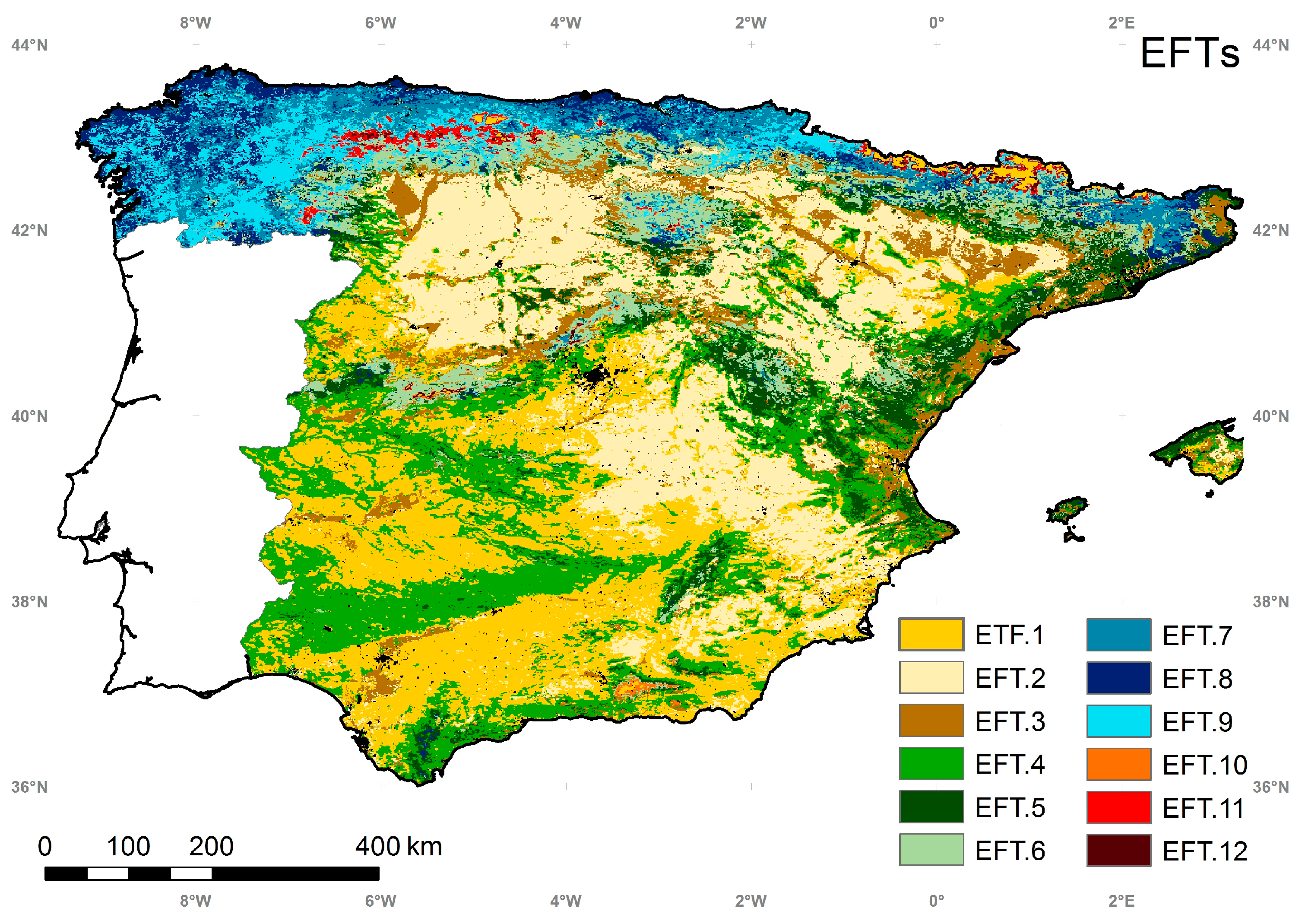
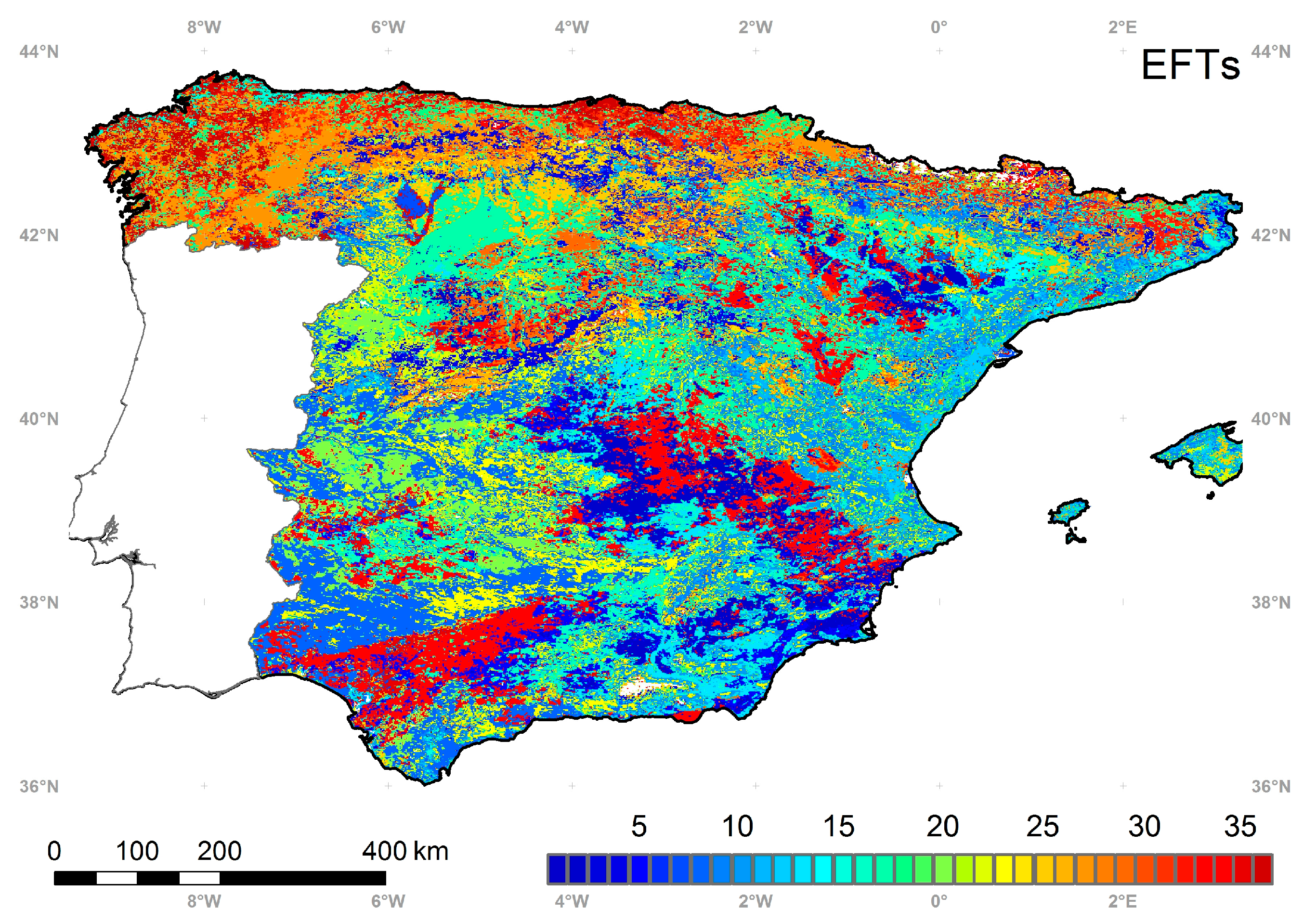
5.4. Ecosystem Functional Types


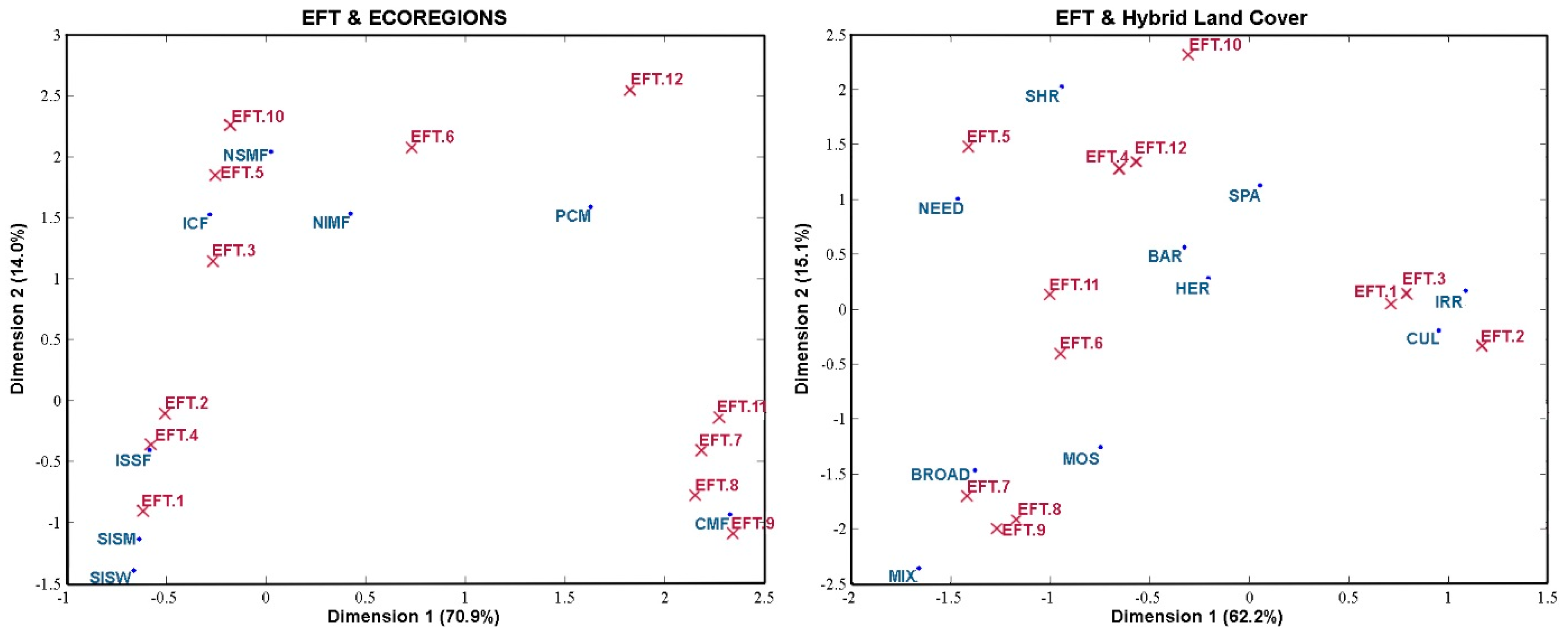
5.5. Intercomparison of the EFTs Map with a Land Cover and Ecoregion Classification
6. Discussion
7. Summary
Acknowledgments
Author Contributions
Conflicts of Interest
References
- Millenium Ecosystem Assessment. Ecosystems and Human Well Being; Island Press: Washington, DC, USA, 2005. [Google Scholar]
- Swift, M.J.; Izac, A.M.N.; Van Noordwijk, M. Biodiversity and ecosystem services in agricultural landscapes—Are we asking the right questions? Agric. Ecosyst. Environ. 2004, 104, 113–134. [Google Scholar] [CrossRef]
- Ayensu, D.V.; Claasen, M.; Collins, A.; Dearing, L.; Fresco, M.; Gadgil, H.; Gitay, G.; Glaser, C.L.; Lohn, J.; Krebs, R.; et al. International ecosystem assessment. Science 1999, 286, 685–686. [Google Scholar] [CrossRef]
- Hill, J.; Stellmes, M.; Udelhoven, T.; Roder, A.; Sommer, S. Mediterranean desertification and land degradation: Mapping related land use change syndromes based on satellite observations. Glob. Planet. Change 2008, 64, 146–157. [Google Scholar] [CrossRef]
- Martínez, B.; Gilabert, M.A. Vegetation dynamics from NDVI time series analysis using the wavelet transform. Remote Sens. Environ. 2009, 113, 1823–1842. [Google Scholar] [CrossRef]
- Baldi, G.; Nosetto, M.D.; Aragón, R.; Aversa, F.; Paruelo, J.M.; Jobbágy, E.G. Long-term satellite NDVI data sets: Evaluating their ability to detect ecosystem functional changes in South America. Sensors 2008, 8, 5397–5425. [Google Scholar] [CrossRef]
- Lambin, E.F.; Geist, H.J.; Lepers, E. Dynamics of land-use and land-cover change in tropical regions. Annu. Rev. Environ. Resour. 2003, 28, 205–241. [Google Scholar] [CrossRef]
- Kaptué-Tchuente, A.; Roujean, J.L.; Faroux, S. ECOCLIMAP-II: An ecosystem classification and land surface parameters database of Western Africa at 1 km resolution for the African Monsoon Multidisciplinary Analysis (AMMA) project. Remote Sens. Environ. 2010, 114, 961–976. [Google Scholar] [CrossRef]
- Fischlin, A.; Midgley, G.F.; Price, J.; Leemans, R.; Brij, G.; Turley, C.; Rounsevell, M.; Dube, P.; Tarazona, J.; Velichko, A. Ecosystems, their properties, goods, and services. In Climate Change 2007: Impacts, Adaptation and Vulnerability: Contribution of Working Group II to the Fourth Assessment Report of the Intergovernmental Panel on Climate Change; Parry, M.L., Canziani, O.F., Palutikof, J.P., van der Linden, P.J., Hanson, C.E., Eds.; Cambridge University Press: Cambridge, UK, 2007; pp. 211–272. [Google Scholar]
- Henle, K.; Alard, D.; Clitherow, J.; Coob, P.; Firbank, L.; Kull, T.; McCracken, D.; Moritz, R.F.A.; Niemelä, J.; Rebane, M.; et al. Identifying and managing the conflicts between agriculture and biodiversity conservation in Europe—A review. Agric. Ecosyst. Environ. 2008, 124, 60–71. [Google Scholar] [CrossRef]
- Cihlar, J. Land cover mapping large areas from satellites: Status and research priorities. Int. J. Remote Sens. 2000, 21, 1093–1114. [Google Scholar] [CrossRef]
- Lhermitte, S.; Verbesselt, J.; Verstraeten, W.W.; Coppin, P.A. Comparison of time series similarity measures for classification and change detection of ecosystem dynamics. Remote Sens. Environ. 2011, 115, 3129–3152. [Google Scholar] [CrossRef]
- Gu, Y.; Brown, J.F.; Miura, T.; Van Leeuwen, W.J.D.; Reed, B.C. Phenological classification of the United States: A geographic framework for extending multi-sensor time-series data. Remote Sens. 2010, 2, 526–543. [Google Scholar] [CrossRef]
- Host, G.E.; Polzer, P.L. A quantitative approach to developing regional ecosystem classifications. Ecol. Appl. 1996, 6, 608–618. [Google Scholar] [CrossRef]
- Waring, R.H.; Coops, N.C.; Fan, W.; Nightingale, J.M. MODIS enhanced vegetation index predicts tree species richness across forested ecoregions in the contiguous USA. Remote Sens. Environ. 2006, 103, 218–226. [Google Scholar] [CrossRef]
- Pérez-Hoyos, A.; Martínez, B.; Gilabert, M.A.; García-Haro, F.J. A multi-temporal analysis of vegetation dynamics in the Iberian peninsula using MODIS-NDVI data. EARSeL eProc. 2010, 9, 22–30. [Google Scholar]
- Huang, C.; Kim, S.; Song, K.; Townshend, J.R.G.; Davis, P.; Altstatt, A.; Rodas, O.; Yanosky, A.; Clay, R.; Tucker, C.J.; et al. Assessment of Paraguay’s forest cover change using Landsat observations. Glob. Planet. Change 2009, 67, 1–12. [Google Scholar] [CrossRef]
- Olson, D.M.; DInersteing, E.; Wikramanayake, E.D.; Burgess, N.D.; Powell, G.V.N.; Underwood, E.C.; D’Amico, J.A.; Itoua, I.; Strand, H.E.; Morrison, J.C.; et al. Terrestrial ecoregions of the world: A new map of life on Earth. Bioscience 2001, 51, 933–938. [Google Scholar] [CrossRef]
- Azzali, S.; Menenti, M. Mapping isogrowth zones on continental scale using temporal Fourier analysis of AVHRR-NDVI data. Int. J. Appl. Earth Obs. Geoinf. 1999, 1, 9–20. [Google Scholar] [CrossRef]
- Soriano, A.; Paruelo, J.M. Biozones: Vegetation units defined by functional characters identifiable with the aid of satellite sensor images. Glob. Ecol. Biogeogr. Lett. 1992, 2, 82–89. [Google Scholar] [CrossRef]
- White, M.A.; Hoffman, F.; Hargrove, W.W.; Nemani, R.R. A global framework for monitoring phenological responses to climate change. Geophys. Res. Lett. 2005, 32, 1–4. [Google Scholar]
- Garbulsky, M.F.; Paruelo, J.M. Remote sensing of protected areas to derive baseline vegetation functioning characteristics. J. Veg. Sci. 2004, 15, 711–720. [Google Scholar] [CrossRef]
- Paruelo, J.M.; Jobbágy, E.G.; Sala, O.E. Current distribution of ecosystem functional types in temperature South America. Ecosystems 2001, 4, 683–698. [Google Scholar] [CrossRef]
- Alcaraz, D.; Cabello, J.; Paruelo, J. Baseline characterization of major Iberian vegetation types based on the NDVI dynamics. Plant Ecol. 2009, 202, 3–29. [Google Scholar]
- Steneck, R.S. Functional groups. In Encyclopedia of Biodiversity; Levin, S.A., Ed.; Academic Press: San Diego, CA, USA, 2001; pp. 21–139. [Google Scholar]
- Virginia, R.A.; Wall, D.H. Principles of ecosystem function. In Encyclopedia of Biodiversity; Levin, S.A., Ed.; Academic Press: San Diego, CA, USA, 2001; pp. 345–352. [Google Scholar]
- Pettorelli, N.; Chauvenet, A.L.M.; Duffy, J.P.; Cornforth, W.A.; Meillere, A.; Baillie, J.E.M. Tracking the effect of climate change on ecosystem functioning using protected areas: Africa as a case study. Ecol. Indic. 2012, 20, 269–276. [Google Scholar] [CrossRef]
- Volante, J.N.; Alcaraz-Segura, D.; Mosciaro, M.J.; Viglizzo, E.F.; Paruelo, J.M. Ecosystem functional changes associated with land clearing in NW Argentina. Agric. Ecosyst. Environ. 2012, 154, 12–22. [Google Scholar] [CrossRef]
- Ivits, E.; Cherlet, M.; Mehl, M.; Sommer, S. Ecosystem functional units characterized by satellite observed phenology and productivity gradients: A case study for Europe. Ecol. Indic. 2013, 27, 17–28. [Google Scholar] [CrossRef]
- Sun, W.; Liang, S.; Xu, G.; Fang, G.; Dickinson, R. Mapping plant functional types from MODIS data using multisource evidential reasoning. Remote Sens. Environ. 2008, 112, 1010–1024. [Google Scholar] [CrossRef]
- Duckworth, J.C.; Kent, M.; Ramsay, P.M. Plant functional types: An alternative to taxonomic plant community description in biogeography? Prog. Phys. Geogr. 2000, 24, 515–542. [Google Scholar] [CrossRef]
- Huete, A.; Liu, H.W.; Batchily, W.; van Leeuwen, W. A comparison of vegetation indices over a global set of TM images for EOS-MODIS. Remote Sens. Environ. 1997, 59, 440–451. [Google Scholar] [CrossRef]
- Julien, Y.; Sobrino, J.A. The Yearly Land Cover Dynamics (YLCD) method: An analysis of global vegetation from NDVI and LST parameters. Remote Sens. Environ. 2009, 113, 329–334. [Google Scholar] [CrossRef]
- Fernández, N.; Paruelo, J.M.; Delibes, M. Ecosystem functioning of protected and altered Mediterranean environments: A remote sensing classification in Doñana, Spain. Remote Sens. Environ. 2010, 114, 211–220. [Google Scholar] [CrossRef]
- Lu, D.; Lueng, Q.W. A survey of image classification methods and techniques for improving classification performance. Int. J. Remote Sens. 2007, 28, 823–870. [Google Scholar] [CrossRef]
- Alcaraz, D.; Paruelo, J.M.; Cabello, J. Identification of current ecosystem functional types in the Iberian Peninsula. Glob. Ecol. Biogeogr. 2006, 15, 200–212. [Google Scholar] [CrossRef]
- Kohonen, T. Self-organized formation of topologically correct feature maps. Biolog. Cybern. 1992, 43, 59–69. [Google Scholar] [CrossRef]
- Kohonen, T. Self-Organizing Maps, 3rd ed.; Springer: Berlin, Germany, 2001. [Google Scholar]
- Vesanto, J.; Himberg, J.; Alhoniemi, E.; Parhankangas, J. SOM Toolbox for Matlab 5; Helsinki University of Technology: Espoo, Finland, 2000. [Google Scholar]
- Gonçalves, M.L.; Netto, M.L.A.; Costa, J.A.F.; Zullo, J.K. An unsupervised method of classifying remotely sensed images using Kohonen self-organizing maps and agglomerative hierarchical clustering methods. Int. J. Remote Sens. 2008, 29, 3171–3207. [Google Scholar] [CrossRef]
- Filippi, A.M.; Jensen, J.R. Fuzzy learning vector quantization for hyperspectral coastal vegetation classification. Remote Sens. Environ. 2006, 100, 512–530. [Google Scholar] [CrossRef]
- Chon, T.S. Self-organizing maps applied to ecological sciences. Ecol. Inform. 2011, 6, 50–61. [Google Scholar] [CrossRef]
- Schmidt, A.; Hanson, C.; Kathilankal, J.; Law, B.E. Classification and assessment of turbulent fluxes above ecosystems in North-America with self-organizing feature map networks. Agric. For. Meteorol. 2011, 151, 508–520. [Google Scholar] [CrossRef]
- Xia, Z.; Rui, S.; Bing, Z.; Qingxi, T. Land cover classification of the North Chinga Plain using MODIS_EVI time series. ISPRS J. Photogramm. 2008, 63, 476–484. [Google Scholar] [CrossRef]
- Del Barrio, G.; Puigdefabregas, J.; Sanjuan, M.E.; Stellmes, M.; Ruiz, A. Assessment and monitoring of land condition in the Iberian Peninsula, 1989–2000. Remote Sens. Environ. 2010, 114, 1817–1832. [Google Scholar] [CrossRef]
- Kerr, J.T.; Ostrovsky, M. From space to species: ecological applications for remote sensing. Trends Ecol. Evol. 2003, 18, 299–305. [Google Scholar] [CrossRef]
- Vermote, E.F.; Vermeulen, A. Atmospheric correction algorithm: Spectral reflectances (MOD09), 1999. NASA-Official Site. Available online: http://modis.gsfc.nasa.gov/data/atbd/atbd_mod08.pdf (accessed on 8 October 2014).
- Huete, H.; Didan, K.; Miura, T.; Rodriguez, E.P.; Gao, X.; Ferreira, L.G. Overview of the radiometric and biophysical performance of the MODIS vegetation indices. Remote Sens. Environ. 2002, 83, 195–213. [Google Scholar] [CrossRef]
- Fensholt, R.; Proud, S.R. Evaluation of earth observation based global long term vegetation trends—Comparing GIMMS and MODIS global NDVI time series. Remote Sens. Environ. 2012, 119, 131–147. [Google Scholar] [CrossRef]
- Benali, A.; Carvalho, A.C.; Nunes, J.P.; Carvalhais, N.; Santos, A. Estimating air surface temperature in Portugal using MODIS LST data. Remote Sens. Environ. 2012, 124, 108–121. [Google Scholar] [CrossRef]
- Mannsteint, H. Surface energy budget, surface temperature and thermal intertia. In Remote Sensing Applications in Meteorology and Climatology; Vaughan, R.A., Reidel, D., Eds.; Springer: Dordrecht, The Netherlands, 1987; pp. 391–410. [Google Scholar]
- Coll, C.; Caselles, V.; Valor, E.; Niclós, R. Comparison between different sources of atmospheric profiles for land surface temperature retrieval from a single channel thermal infrared data. Remote Sens. Environ. 2012, 117, 199–210. [Google Scholar] [CrossRef]
- Wan, Z.; Zhang, Y.; Li, Z.; Wang, R.; Salomonson, V.V.; Yves, A.; Bosseno, R.; Hanocq, J.F. Preliminary estimate of calibration of the moderate resolution imaging spectroradiometer thermal infrared data using Lake Titicaca. Remote Sens. Environ. 2002, 80, 497–515. [Google Scholar] [CrossRef]
- Wang, W.; Liang, S.; Meyers, T. Validating MODIS land surface temperature products using long-term nighttime ground measurements. Remote Sens. Environ. 2008, 112, 623–635. [Google Scholar] [CrossRef]
- Román, M.O.; Schaaf, C.B.; Woodcok, C.E.; Strahler, A.H.; Yang, X.; Braswell, R.H.; Curtis, P.S.; Davis, K.J.; Dragoni, D.; Goulden, M.L.; et al. The MODIS (Collection V005) BRDF/albedo product: Assessment of spatial representativeness over forested landscapes. Remote Sens. Environ. 2009, 113, 2476–2498. [Google Scholar] [CrossRef]
- Sellers, P.J.; Hall, F.G.; Kelly, R.D.; Black, A.; Baldocchi, D.; Berry, J. BOREAS in 1997: Experiment overview, scientific results, and future directions. J. Geophys. Res. Atmos. 1997, 102, 28731–28769. [Google Scholar] [CrossRef]
- Dickinson, R.E. Land surface processes and climate surface albedos and energy-balance. Adv. Geophys. 1983, 25, 305–353. [Google Scholar]
- Lawrence, D.M.; Slingo, J.M. An annual cycle of vegetation in GCM. Part II: Global impacts on climate and hydrology. Clim. Dyn. 2004, 22, 107–122. [Google Scholar] [CrossRef]
- Wang, S.; Grant, R.F.; Verseghy, D.L.; Black, T.A. Modelling carbon dynamics of boreal forest ecosystems using the Canadian Land Surface Scheme. Clim. Change 2002, 55, 451–477. [Google Scholar] [CrossRef]
- Jin, Y.; Schaaf, C.B.; Woodcock, F.; Gao, X.; Li, A.H.; Strahler, A.H.; Lucht, W.; Liang, S. Consistency of MODIS surface bidirectional reflectance distribution function and albedo retrievals: 2. Validation. J. Geophys. Res. 2003, 108, 1984–2012. [Google Scholar]
- Liang, S.L.; Fang, H.L.; Chen, M.Z.; Shuey, C.J.; Walthall, C.; Daughtry, C. Validating MODIS land surface reflectance and albedo products: Methods and preliminary results. Remote Sens. Environ. 2002, 83, 149–162. [Google Scholar] [CrossRef]
- Salomon, J.G.; Crystal, C.B.; Strahler, A.H.; Gao, F.; Jin, Y. Validation of the MODIS bidirectional reflectance distribution function and albedo retrievals using combined observations from the aqua and terra platforms. IEEE Trans. Geosci. Remote Sens. 2006, 44, 1555–1565. [Google Scholar] [CrossRef]
- Matheron, G. Principles of geostatistics. Econ. Geol. 1963, 58, 1246–1266. [Google Scholar] [CrossRef]
- Cressie, N. The origins of kriging. Math. Geol. 1990, 2, 239–253. [Google Scholar] [CrossRef]
- Savitzky, A.; Golay, M.J.E. Smoothing and differentiation of data by simplified least squares procedures. Anal. Chem. 1964, 36, 1627–1639. [Google Scholar] [CrossRef]
- Holben, B.N. Characteristics of maximum-value composite images for temporal AVHRR data. Int. J. Remote Sens. 1986, 7, 1435–1445. [Google Scholar] [CrossRef]
- Hird, J.; McDermid, G.J. Noise reduction of NDVI time series: An empirical comparison of selected techniques. Remote Sens. Environ. 2009, 113, 248–258. [Google Scholar] [CrossRef]
- Chen, J.; Jönsson, P.; Tamura, M.; Gu, Z.; Matsushita, B.; Eklundh, L. A simple method for reconstructing a high-quality NDVI time-series data set based on the Savitzky-Golay filter. Remote Sens. Environ. 2004, 91, 332–344. [Google Scholar] [CrossRef]
- Ren, J.; Chen, Z.; Zhou, Q.; Tang, H. Regional yield estimation for winter wheat with MODIS-NDVI data in Shandong, China. Int. J. Appl. Earth Obs. Geoinf. 2008, 10, 403–413. [Google Scholar] [CrossRef]
- Wang, Q.; Zhao, P.; Ren, H.; Kakubari, Y. Spatiotemporal dynamics of forest net primary production in China over the past two decades. Glob. Planet. Change 2008, 61, 267–274. [Google Scholar] [CrossRef]
- García-Haro, F.J.; Belda, F; Gilabert, M.A.; Meliá, J.; Moreno, A.; Poquet, D.; Pérez-Hoyos, A.; Segarra, D. Monitoring drought conditions in the Iberian Peninsula using moderate and coarse resolution satellite data. In Proceedings of the 2nd MERIS/(A)ATSR User Workshop’, Frascaty, Italy, 22–26 September 2008.
- Thornthwaite, C.W. An approach toward a rational classification of climate. Geogr. Rev. 1948, 38, 55–94. [Google Scholar] [CrossRef]
- Kohonen, T. The self-organizing map. Neurocomputing 1998, 21, 1–6. [Google Scholar] [CrossRef]
- Ghaseminezhad, M.H.; Karami, A. A novel self-organizing map (SOM) neural network for discrete groups of data clustering. Appl. Soft Comput. 2011, 11, 3771–3778. [Google Scholar] [CrossRef]
- Xu, R.; Wunsch, D. Survey of clustering algorithms. IEEE Trans. Neural Netw. 2005, 16, 645–678. [Google Scholar] [CrossRef] [PubMed]
- Kiviluoto, K. Topology preservation in self-organizing maps. In Proceedings of the IEEE International Conference on Neural Networks, Washington, DC, USA, 3–6 June 1996; 1996; pp. 294–299. [Google Scholar]
- MacQueen, J.B. Some methods for classification and analysis of multivariate observations. In Proceedings of the Fifth Berkeley Symposium on Mathematical Statistic and Probability, Berkeley, CA, USA, 21 June–18 July 1965, 27 December 1965–7 January 1966.
- Maulik, U. Performance evaluation of some clustering algorithms and validity indices. IEEE Trans. Pattern Anal. Mach. Intell. 2002, 24, 1650–1654. [Google Scholar] [CrossRef]
- Davies, D.L.; Bouldin, D.W. A cluster separation measure. IEEE Trans. Pattern Anal. Mach. Intell. 1979, 1, 224–227. [Google Scholar] [CrossRef] [PubMed]
- Petrovic, S. A comparison between the silhouette index and the Davies-Bouldin index in labeling ids clusters. In Proceedings of the 11th Nordic Workshop of Secure IT Systems, Linköping, Sweden, 19–20 October 2006.
- Zavala, L.M.; González, F.A.; Jordán, A. Intensity and persistence of water repellence in relation to vegetation types and soil parameters in Mediterranean SW Spain. Geoderma 2009, 152, 361–374. [Google Scholar] [CrossRef]
- Benavides, R.; Montes, F.; Rubio, A.; Osoro, K. Geostatistical modelling of air temperature in a mountainous region of Northern Spain. Agric. For. Meteorol. 2007, 146, 173–188. [Google Scholar] [CrossRef]
- Liang, S. Narrowband to broadband conversions of land surface albedo I: Algorithms. Remote Sens. Environ. 2001, 76, 213–238. [Google Scholar] [CrossRef]
- Vicente-Serrano, S.M.; Cuadrat-Prats, J.M.; Romo, A. Aridity influence on vegetation patterns in the middle Ebro Valley (Spain): Evaluation by means of AVHRR images and climate interpolation techniques. J. Arid Environ. 2006, 66, 353–375. [Google Scholar] [CrossRef]
- Tabari, H.; Talaee, H.P. Moisture index for Iran: Spatial and temporal analysis. Glob. Planet. Change 2013, 100, 11–19. [Google Scholar] [CrossRef]
- Gao, X.; Giorgi, F. Increased aridity in the Mediterranean region under greenhouse gas forcing estimated from high resolution simulations with a regional climate model. Glob. Planet. Change 2008, 62, 195–209. [Google Scholar] [CrossRef]
- Kamimura, R. Supposed maximum information for comprehensible representations in SOM. Neurocomputing 2011, 74, 1116–1134. [Google Scholar] [CrossRef]
- Naldi, M.C.; Campello, R.J.; Hruschka, E.R.; Carvalho, A.C. Efficiency issues of evolutionary k-means. Appl. Soft Comput. 2011, 11, 1938–1952. [Google Scholar] [CrossRef]
- Moreno, A. Retrieval and Assessment of CO2 Uptake by Mediterranean Ecosystems Using Remote Sensing and Meteorological Data. Ph.D. Thesis, University of Valencia, Valencia, Spain, 2014. [Google Scholar]
- Wilks, S.S. On the independence of k sets of normally distributed statistical variables. Econom. J. Econom. Soc. 1935, 3, 309–326. [Google Scholar]
- Pérez-Hoyos, A.; García-Haro, F.J.; San-Miguel-Ayanz, J. Conventional and fuzzy comparisons of large scale land cover products: Application to CORINE, GLC2000, MODIS and GlobCover in Europe. ISPRS J. Photogramm. Remote Sens. 2012, 74, 185–201. [Google Scholar] [CrossRef]
- Benzécri, J.P. L’analyse des correspondences. In L’Analyse Des Données; Dunod: Paris, France, 1973. [Google Scholar]
- Minnick, R.F. A method for the measurement of areal correspondence. Mich. Acad. Sci. Arts Lett. 1964, 49, 333–343. [Google Scholar]
- Cabello, J.; Fernández, N.; Alcaraz-Segura, D.; Oyonarte, C.; Piñero, G.; Altesor, A.; Delibes, M.; Paruelo, J.M. The ecosystem functioning dimension in conservation: Insights from remote sensing. Biodivers. Conserv. 2012, 21, 3287–3305. [Google Scholar] [CrossRef] [Green Version]
- Alcaraz-Segura, D.; Paruelo, J.M.; Epstein, H.E.; Cabello, J. Environmental and human controls of ecosystem functional diversity in temperate South America. Remote Sens. 2013, 5, 127–154. [Google Scholar] [CrossRef]
Appendix


| Variable | Wilk’s Lambda |
|---|---|
| Moisture | 0.24913 |
| IAlbedo | 0.27629 |
| Aridity Index | 0.29232 |
| ValminNDVI | 0.3122 |
| ValmaxLst | 0.33468 |
| INDVI | 0.33787 |
| DNDVI | 0.34857 |
| ValmeanLST | 0.37458 |
| ValminAlbedo | 0.397 |
| DAlbedo | 0.51617 |
| DLST | 0.51617 |
| RelNDVI | 0.78532 |
| EFT.1 | EFT.2 | EFT.3 | EFT.4 | EFT.5 | EFT.6 | EFT.7 | EFT.8 | EFT.9 | EFT.10 | EFT.11 | EFT.12 | |
|---|---|---|---|---|---|---|---|---|---|---|---|---|
| Irrigated | 0.03 | 0.04 | 0.23 | 0.01 | 0.00 | 0.01 | 0.00 | 0.00 | 0.00 | 0.00 | 0.00 | 0.00 |
| Cultivated | 0.37 | 0.64 | 0.09 | 0.06 | 0.01 | 0.03 | 0.01 | 0.01 | 0.01 | 0.00 | 0.00 | 0.00 |
| Mosaic Cultivated | 0.04 | 0.02 | 0.02 | 0.04 | 0.03 | 0.08 | 0.07 | 0.06 | 0.09 | 0.00 | 0.01 | 0.00 |
| Broadleaved | 0.01 | 0.00 | 0.01 | 0.08 | 0.04 | 0.10 | 0.15 | 0.07 | 0.12 | 0.00 | 0.01 | 0.00 |
| Needleleaved | 0.01 | 0.00 | 0.01 | 0.10 | 0.28 | 0.09 | 0.07 | 0.06 | 0.03 | 0.00 | 0.01 | 0.00 |
| Mixed Forest | 0.00 | 0.00 | 0.00 | 0.02 | 0.05 | 0.04 | 0.09 | 0.11 | 0.10 | 0.00 | 0.01 | 0.00 |
| Shrublands | 0.03 | 0.00 | 0.02 | 0.21 | 0.11 | 0.05 | 0.02 | 0.01 | 0.03 | 0.00 | 0.01 | 0.00 |
| Herbaceous | 0.12 | 0.03 | 0.05 | 0.14 | 0.01 | 0.04 | 0.05 | 0.03 | 0.04 | 0.00 | 0.01 | 0.01 |
| Sparse | 0.07 | 0.03 | 0.04 | 0.08 | 0.03 | 0.04 | 0.00 | 0.00 | 0.01 | 0.01 | 0.02 | 0.02 |
| Bare | 0.00 | 0.00 | 0.00 | 0.00 | 0.00 | 0.00 | 0.00 | 0.00 | 0.00 | 0.01 | 0.01 | 0.01 |
| Wetlands | 0.00 | 0.00 | 0.00 | 0.00 | 0.00 | 0.00 | 0.00 | 0.00 | 0.00 | 0.01 | 0.00 | 0.00 |
| Snow | 0.00 | 0.00 | 0.00 | 0.00 | 0.00 | 0.00 | 0.00 | 0.00 | 0.00 | 0.00 | 0.00 | 0.00 |
| EFT.1 | EFT.2 | EFT.3 | EFT.4 | EFT.5 | EFT.6 | EFT.7 | EFT.8 | EFT.9 | EFT.10 | EFT.11 | EFT.12 | |
|---|---|---|---|---|---|---|---|---|---|---|---|---|
| Cantabrian Mixed Forest | 0.00 | 0.00 | 0.01 | 0.00 | 0.00 | 0.08 | 0.36 | 0.26 | 0.37 | 0.00 | 0.03 | 0.01 |
| Pyrenees Conifer | 0.01 | 0.00 | 0.00 | 0.00 | 0.01 | 0.09 | 0.09 | 0.03 | 0.03 | 0.00 | 0.05 | 0.08 |
| Iberian Conifer | 0.03 | 0.07 | 0.06 | 0.05 | 0.09 | 0.08 | 0.00 | 0.00 | 0.00 | 0.02 | 0.00 | 0.00 |
| Iberian Sclerophyllous | 0.40 | 0.39 | 0.08 | 0.26 | 0.06 | 0.02 | 0.00 | 0.00 | 0.00 | 0.00 | 0.00 | 0.00 |
| Northeastert Mediterranean Forest | 0.01 | 0.01 | 0.14 | 0.06 | 0.18 | 0.03 | 0.04 | 0.03 | 0.00 | 0.00 | 0.00 | 0.00 |
| Northwest Iberian Montane | 0.02 | 0.08 | 0.06 | 0.03 | 0.05 | 0.21 | 0.03 | 0.03 | 0.06 | 0.00 | 0.01 | 0.00 |
| Southeastern IberainShrubs | 0.01 | 0.01 | 0.00 | 0.00 | 0.00 | 0.00 | 0.00 | 0.00 | 0.00 | 0.00 | 0.00 | 0.00 |
| Southwest Iberian Sclerophyllous | 0.12 | 0.01 | 0.03 | 0.11 | 0.02 | 0.00 | 0.00 | 0.00 | 0.00 | 0.00 | 0.00 | 0.00 |
© 2014 by the authors; licensee MDPI, Basel, Switzerland. This article is an open access article distributed under the terms and conditions of the Creative Commons Attribution license (http://creativecommons.org/licenses/by/4.0/).
Share and Cite
Pérez-Hoyos, A.; Martínez, B.; García-Haro, F.J.; Moreno, Á.; Gilabert, M.A. Identification of Ecosystem Functional Types from Coarse Resolution Imagery Using a Self-Organizing Map Approach: A Case Study for Spain. Remote Sens. 2014, 6, 11391-11419. https://doi.org/10.3390/rs61111391
Pérez-Hoyos A, Martínez B, García-Haro FJ, Moreno Á, Gilabert MA. Identification of Ecosystem Functional Types from Coarse Resolution Imagery Using a Self-Organizing Map Approach: A Case Study for Spain. Remote Sensing. 2014; 6(11):11391-11419. https://doi.org/10.3390/rs61111391
Chicago/Turabian StylePérez-Hoyos, Ana, Beatriz Martínez, Francisco Javier García-Haro, Álvaro Moreno, and María Amparo Gilabert. 2014. "Identification of Ecosystem Functional Types from Coarse Resolution Imagery Using a Self-Organizing Map Approach: A Case Study for Spain" Remote Sensing 6, no. 11: 11391-11419. https://doi.org/10.3390/rs61111391