DEnKF–Variational Hybrid Snow Cover Fraction Data Assimilation for Improving Snow Simulations with the Common Land Model

Abstract

This study assesses the analysis performance of a hybrid DEnKF-variational data assimilation (DA) method (DEnVar) for assimilating the MODIS snow cover fraction (SCF) into the Common Land Model (CoLM). Coupling a deterministic ensemble Kalman filter (DEnKF) with a one-dimensional variational DA method (1DVar), DEnVar without observation perturbations is a two-step DA method. That is, the analysis ensemble mean and analysis error covariance of DEnKF are introduced into the 1DVar hybrid cost function, and the analysis mean of DEnKF is replaced by the 1DVar analysis. The analysis performance of DEnVar was experimentally compared with DEnKF, 1DVar, and EnVar (hybrid ensemble-variational DA) at five sites in the Altay region of China from November 2008 to March 2009. From our results, it is shown that the four DA experiments can improve snow simulations at most sites when the available MODIS SCF is assimilated. The DEnVar experiment using the hybrid error covariance shows the best analysis performance among the four DA experiments at most sites. Furthermore, sensitivity tests show that DEnVar is slightly sensitive to the weighting coefficient, which controls the respective weights of ensemble- and (National Meteorological Center) NMC-based error covariances, but is highly sensitive to the observation error. DEnVar obtains better analysis performance when using the ensemble-based analysis error covariance rather than the hybrid error covariance coupling ensemble-based analysis and static NMC-based error covariances. The inaccurate distribution of observation error may invalidate the DEnVar method.

1. Introduction

Seasonal snow cover plays a crucial role in the Earth’s hydrological processes, land surface energy balance, and climate [1,2,3] due to its high albedo and low thermal conductivity [4,5]. The snow cover fraction (SCF) is a key parameter in the studies of both hydrology and climatology [6]. Normally, SCF is derived from snowpack state such as snow depth (SD) or snow water equivalent (SWE). SD and SWE are important internal variables of hydrological and climatic models. SWE is the product of SD and snow density. They have significant impacts on climatic and hydrological simulations and snowmelt runoff predictions [7]. Substantial snow accumulation frequently causes severe snow disasters, such as frostbite, death for both animals and people, and traffic disruption [8]. Massive and rapid snowmelt may cause flooding. Therefore, the accurate estimates of SD and SWE are important for reduction, mitigation, and prevention of snow-related disasters [9].

To improve the SD and SWE estimates, some substantial efforts have been made through data assimilation (DA) to explore optimal combinations of physical models and snow-related observations. Most studies have mainly used rule-based direct insertion (e.g., [10,11,12,13]), ensemble-based (e.g., ensemble Kalman filter (EnKF) [14,15,16,17], ensemble square root filter (EnSRF) [18], ensemble adjustment Kalman filter (EAKF) [19], and deterministic ensemble Kalman filter (DEnKF) [20]), or Bayesian (e.g., [21,22,23]) DA methods to assimilate SCF (e.g., [24,25]), SWE (e.g., [5,16,26]), SD [12], or passive microwave brightness temperature [27] observations into hydrological and land surface models to improve snow estimates. All existing studies show that these DA methods improve the SD and SWE estimates when available snow-related observations are assimilated into hydrological and land surface models.

In recent decades, a hybrid DA method of utilizing advanced features of both ensemble-based and variational DA methods has been proposed (e.g., [28,29,30,31,32]) for numerical weather prediction (e.g., [33,34,35,36]). For the hybrid method, the ensemble covariance generated from the ensemble-based DA system is easily incorporated into the hybrid cost function of variational DA. The hybrid DA system can conform well to the existing variational framework and be more flexible than the conventional ensemble-based methods for exploring sampling errors and model errors [36]. Recent studies have also demonstrated the potential of the hybrid method as compared with the stand-alone EnKF and variational methods (e.g., [32,37,38]).

Given that these hybrid DA methods have been successfully used for improving numerical weather prediction, we hypothesize that a hybrid DA method is certainly beneficial to snow simulations. The stochastic EnKFs refer to perturbing observations for exploring observation uncertainties [39], which may introduce sampling errors and lead to non-optimal DA, especially for small ensembles [40]. In the SCF assimilation, perturbing the full SCF observations may decrease the SCF observations, and therefore systematically and substantially underestimate the SWE [15]. A feasible alternative to ensemble square root filter (EnSRF) [41] that has been developed is a relatively robust deterministic ensemble Kalman filter (DEnKF) without observation perturbations. As compared with the EnSRF [42], the DEnKF is easier to implement. The DEnKF method has been used to assimilate MODIS SCF into the Common Land Model (CoLM) for SD simulation improvements. However, the assimilated results have shown that the assimilation of MODIS SCF only using the DEnKF method (a sample ensemble size of 30) cannot effectively improve SD simulations [20]. To avoid underestimation of analysis ensemble mean and background error covariance of DEnKF with smaller ensembles, a hybrid method (DEnVar) of DEnKF-variational DA without observation perturbations that couples DEnKF and 1DVar methods is proposed to assimilate MODIS SCF observations into the CoLM for improving SD and SWE simulations. As a comparison with the other three DA methods—DEnKF, 1DVar, and EnVar (hybrid ensemble-variational DA)—the DEnVar method was used at five sites in the Altay region of China from November 2008 to March 2009. The EnVar method is similar to the method of Zhang et al. [36]. We performed sensitivity tests on the hybrid error covariance weight and the observation errors.

The CoLM and related data assimilation methods are described in Section 2. The experimental design and data sets are introduced in section 3. Section 4 presents a comparison of DEnVar and other DA methods and sensitivity tests on DEnVar. Concluding remarks are given in Section 5.

2. Methods

2.1. Common Land Model

A column (1-D) model, the Common Land Model (CoLM), is the latest land surface model for climate studies [43]. The CoLM combines the advanced features of three outstanding and well-documented land surface models, including the Land Surface Model (LSM) [44], the Biosphere-Atmosphere Transfer Scheme (BATS) [45], and the 1994 version of the Chinese Academy of Science Institute of Atmospheric Physics LSM (IAP94) [46]. In the CoLM, SD and SWE are forecast variables. As a diagnostic variable, snow cover calculated by total SD directly affects energy fluxes and grid-averaged albedo in the CoLM. The CoLM has the five-layer snow scheme which accounts for layer-based liquid water retention, thawing-freezing, snow-melt, and heat energy. Snow compaction accounts for the destructive, pressure, and melt metamorphisms. At each time step, snow layers can be combined or divided in terms of the snow accumulation or melting conditions, like layer thicknesses. More details about snow processes in the CoLM can be found in the works of Dai et al. [47] and Dai et al. [43].

2.2. Variational Method

In traditional variational assimilation, the analysis is performed by minimizing a cost function J [28]:

(1)

where x = [snowdp, swe] stands for the analysis state vector (e.g. snow depth and snow water equivalent in the CoLM), and x^b for the background state vector. B stands for the static background error covariance matrix, y^o for the MODIS SCF observation vector, R for the error variance of MODIS SCF observations, and H for the nonlinear observation operator mapping model variables to observation variables. A snow cover depletion curve (SDC) that parameterizes the relationship between SD and SCF in the CoLM is considered as the observation operator of snow DA [45]:

$$SC{F}^{\prime }=H(x)=\frac{snowdp}{10z_{0g}+snowdp}$$

(2)

where $SC{F}^{\prime }$ stands for the predicted SCF observation, snowdp for the CoLM simulated snow depth, and z_0g for the roughness length for bare soil with a default value of 0.01 m.

By defining the analysis increment $\delta x=x-x^b$ and linearizing H(x) about x^b, Equation (1) is rewritten as follows [48]:

(3)

where $d=y^o-H\left(x^b\right)$ stands for the innovation vector, and $H=\partial H/\partial x$ at x^b for the Jacobian matrix of the nonlinear observation operator H.

The gradient of the cost function from Equation (3) with respect to $\delta x$ is given as follows:

∇J (δx) = (B⁻¹ + H^T R⁻¹H) δx − H^T R⁻¹d

(4)

Next, we convert a minimum function problem into a problem of finding the solution of $\nabla J\left(\delta x\right)$. The conjugate-gradient method, which offers a good tradeoff between convergence rates and computer memory requirements, is used to minimize the quadratic cost function in our work.

2.3. Deterministic Ensemble Kalman Filter

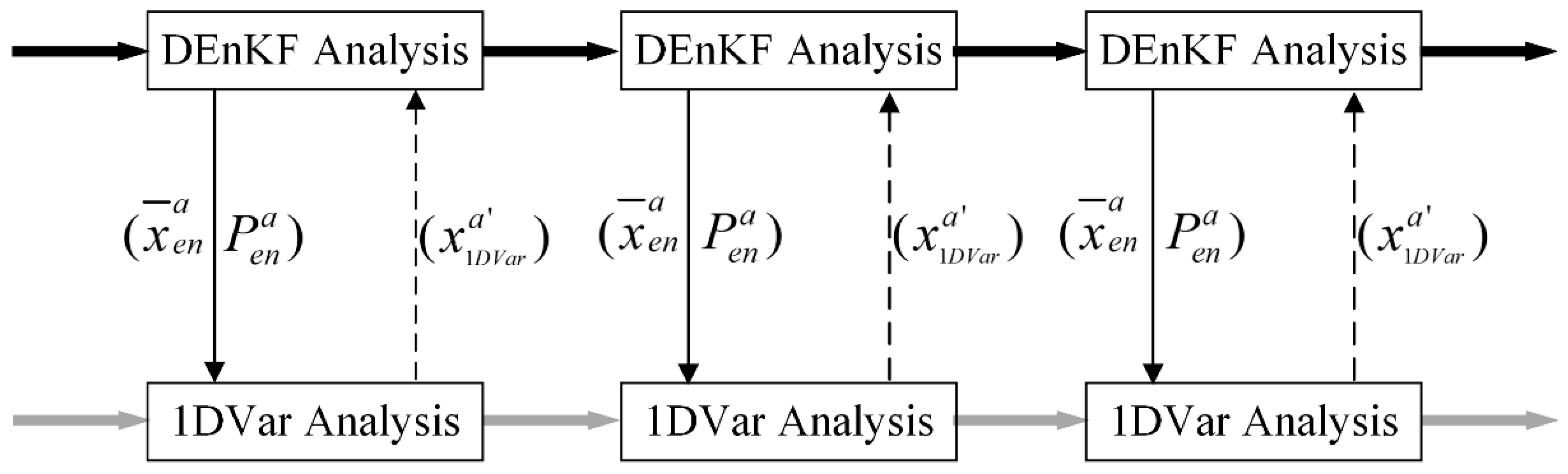
Without observation perturbations, a deterministic ensemble Kalman filter (DEnKF) has been proposed by Sakov and Oke [41]. The updated equations of the DEnKF are given as follows:

$${\overline{x}}^a={\overline{x}}^b+K[y^o-H({\overline{x}}^b)]$$

(5)

$${\overline{x}}^b=\frac{1}{\mathrm{N}}\sum _{i=1}^N{\mathrm{ x}}_i^b$$

(6)

K = P^bH^T (HP^bH^T + R)⁻¹

(7)

(8)

where ${\overline{x}}^a=\left[{\overline{snowdp}}^a, {\overline{swe}}^a\right]$ and ${\overline{x}}^b$ stand for the analysis and background ensemble means of snow depth (snowdp) and snow water equivalent (swe) states, $x_i^b=\left[snowd{p}_i^b,sw{e}_i^b\right]$ for the CoLM simulated snow state, i for the ensemble index, and N for the ensemble size. K stands for the Kalman gain matrix and y° for the MODIS SCF observation. Here the MODIS SCF observation is not perturbed. H stands for an observation operator as Equation (2). P^b stands for the background error covariance matrix and R for the error variance of MODIS SCF observations. $A^b=\left[x_1^b-{\overline{x}}^b,x_2^b-{\overline{x}}^b,\cdots ,x_N^b-{\overline{x}}^b\right]$ stands for the background ensemble perturbation.

The DEnKF maintains the ensemble spread by halving the Kalman gain in the analysis perturbation update stage. That is,

$$A^a=A^b-\frac{1}{2}KH{A}^b$$

(9)

where A^a stands for the analysis ensemble perturbation. This formulation can be thought of as an inherent covariance inflation similar to the relaxation-to-prior algorithm of Zhang et al. [49]. The covariance inflation can avoid the collapse of ensemble spread and further reduce the risk of filter divergence [41,50].

Finally, the analysis ensemble is generated by adding perturbations to the analysis ensemble mean. It is denoted by

$$X^a=A^a+{[{\overline{x}}^a,\dots ,{\overline{x}}^a]}_{.}$$

(10)

2.4. Coupled Method

For snow data assimilation (DA), a two-way coupled DEnKF-1DVar hybrid method (DEnVar) patterned after Zhang et al. [36] is proposed. Two-way coupling re-centers the DEnKF analysis ensemble mean with the 1DVar analysis. Such re-centering may help to prevent the divergence of the DEnKF analyses so that the ensemble perturbations empirically represent the distribution of the forecast errors. Unlike the EnVar method (hybrid ensemble-variational DA) of Zhang et al. [36], the two-step DEnVar method without observation perturbations in Figure 1 includes three steps: (1) the DEnKF analysis is implemented to generate the analysis ensemble mean ${\overline{x}}_{en}^a$ and the analysis error covariance $P_{en}^a$, (2) the analysis ensemble mean ${\overline{x}}_{en}^a$ is used as the first guess for the 1DVar and the analysis error covariance $P_{en}^a$ is introduced into the 1DVar hybrid cost function, and (3) the analysis ensemble mean ${\overline{x}}_{en}^a$ of DEnKF is replaced with the 1DVar analysis for the next ensemble forecast.

Figure 1. A hybrid analysis method of DEnVar which couples the DEnKF and the 1DVar.

Figure 1. A hybrid analysis method of DEnVar which couples the DEnKF and the 1DVar.

The hybrid error covariance is included in the hybrid cost function by separating the J_b in Equation (1) into two parts [28,51]:

(11)

where J_b1 stands for the traditional 1DVar background term as in Equation (1) and J_b2 for the ensemble-based term. B_NMC stands for the static background error covariance calculated by the NMC (National Meteorological Center) method [52], and $P_{en}^a$ for the analysis error covariance valid at the time of analysis. β stands for the weighting coefficient that is used to control the respective weights of static NMC-based background and ensemble-based analysis error covariances. If β approaches 0, then the hybrid formulation is functionally equivalent to the standard 1DVar method. If β is 1, the hybrid error covariance only contains the ensemble-based analysis error covariance. If β is nonzero, then the hybrid method takes the mixed value of both static NMC and ensemble-based error covariances.

2.5. Error Evaluation Methods

To evaluate the analysis performance of these assimilation methods, we selected three indices of bias, root mean squared error (RMSE), and normalized error reduction percent (NERP) [53] as follows:

$$Bias=\frac{\sum _{i=1}^n(y_{s,i}-y_{o,i})}{n}$$

(12)

$$RMSE=\sqrt{\frac{\sum _{i=1}^n{(y_{s,i}-y_{o,i})}^2}{n}}$$

(13)

$$NERP=(1-\frac{RMS{E}_a}{RMS{E}_s})\times 100\%$$

(14)

where y_s,i and y_o,i stand for the i-th simulated (simulation without assimilation or assimilation) and observed snow states, respectively, and n for the number of time points. The NERP index is used to measure the improved magnitudes of these assimilation methods. RMSE_s and RMSE_a are the root-mean square errors of simulated and analyzed snow states, respectively. NERP ranges from negative infinity to 100%, where 100% means that the assimilated results are identical to the observations. A negative NERP represents a percent of deterioration for the analyzed states as compared with the simulations without DA.

3. Experimental Design and Data Sets

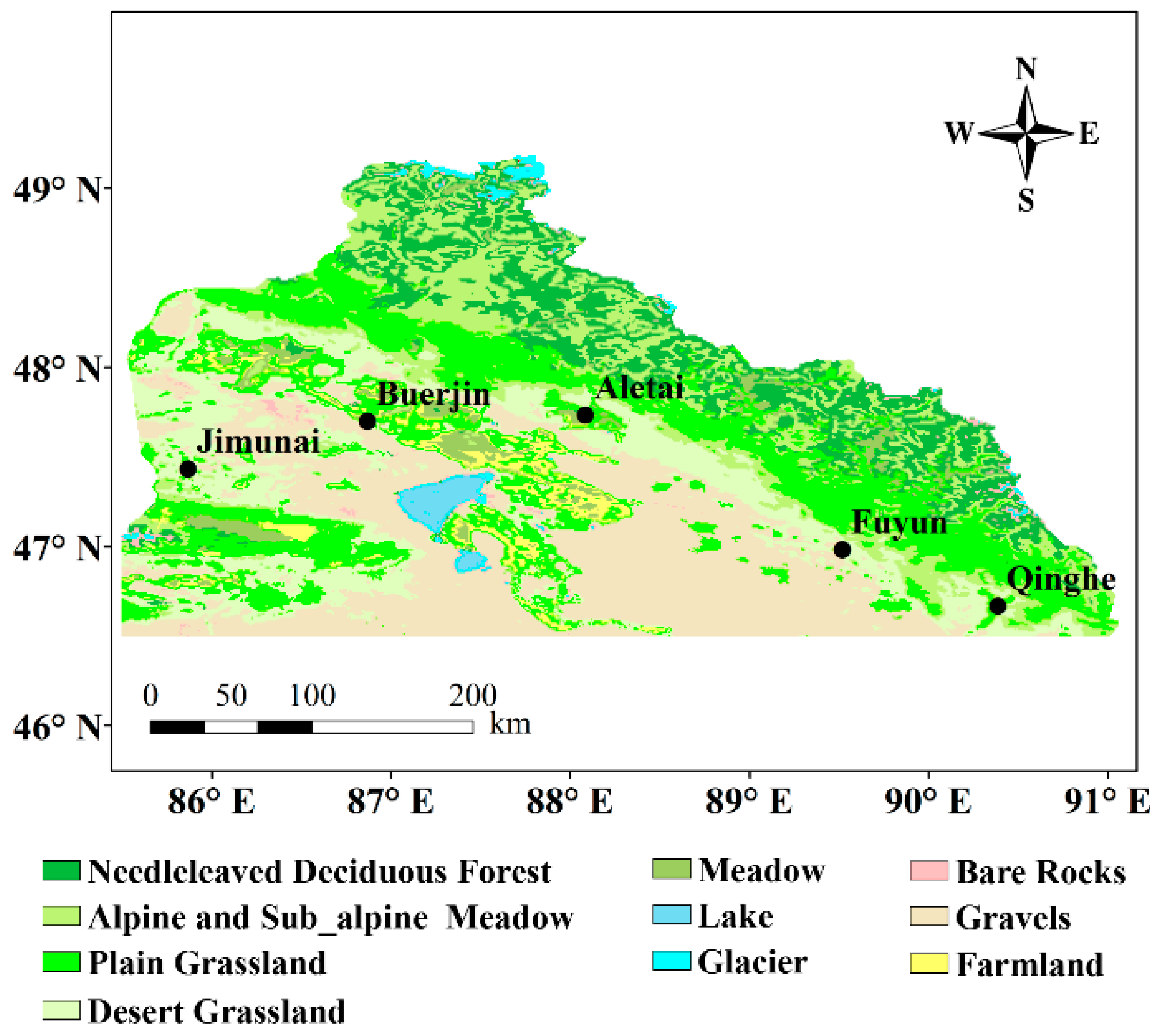
3.1. Experimental Sites

The snow DA methods were used at five sites in the Altay region of Northern Xinjiang, China (Figure 2). These five sites are located in a homogeneous land cover area. The geographic locations and elevations of five sites are given in Table 1. Influenced by the Siberian High, these five sites experience a long, cold and snowy winter. This leads to an approximate 120-day duration of snow cover from November to March of the next year [54]. Only the daily in situ SD and air temperature measurements were collected at all sites from January 2004 to March 2009. Huang et al. [54] and Xu and Shu [20] have pointed out that it is feasible to compare in situ SD observations with MODIS snow cover or the CoLM-simulated SD over a variety of environmental conditions. For example, it is possible to make a comparison between in situ SD observations and the CoLM-simulated SD with a 0.01° spatial resolution. In situ SD observations from November 2008 to March 2009 were considered as validation data sets for assessing the performance of snow DA methods. The mean SDs at five sites during this period are shown in Table 1.

Table 1. Characteristics of five sites in the Altay region of China. The mean SD is calculated from daily in situ SD observations from November 2008 to March 2009, and the mean SWE is calculated by daily AMSR-E retrieved SWE from November 2008 to March 2009. The term “Pairs” implies the valid pairs of 48-h and 24-h CoLM snow forecasts from November 2007 to March 2008. The number (Num) of nonzero snow observations was calculated during the period of January 2004 to October 2008. The observation standard error (σ_obs) is calculated by fitting MODIS SCF observations to AMSR-E SWE-based SCF observations.

Site	Lon	Lat	Elevation (m)	Mean SD (cm)	Mean SWE (mm)	Pairs	Num	σobs (%)
Aletai	88.083	47.733	737	32.71	88.53	86	253	27.75
Buerjin	86.867	47.400	456	15.41	26.84	80	125	27.78
Fuyun	89.517	46.983	826	15.99	69.77	91	206	22.85
Jimunai	85.867	47.433	984	22.80	36.68	83	248	28.56
Qinghe	90.383	46.667	1 200	14.35	61.37	96	175	29.70

Table 1. Characteristics of five sites in the Altay region of China. The mean SD is calculated from daily in situ SD observations from November 2008 to March 2009, and the mean SWE is calculated by daily AMSR-E retrieved SWE from November 2008 to March 2009. The term “Pairs” implies the valid pairs of 48-h and 24-h CoLM snow forecasts from November 2007 to March 2008. The number (Num) of nonzero snow observations was calculated during the period of January 2004 to October 2008. The observation standard error (σ_obs) is calculated by fitting MODIS SCF observations to AMSR-E SWE-based SCF observations.

Site	Lon	Lat	Elevation (m)	Mean SD (cm)	Mean SWE (mm)	Pairs	Num	σobs (%)
Aletai	88.083	47.733	737	32.71	88.53	86	253	27.75
Buerjin	86.867	47.400	456	15.41	26.84	80	125	27.78
Fuyun	89.517	46.983	826	15.99	69.77	91	206	22.85
Jimunai	85.867	47.433	984	22.80	36.68	83	248	28.56
Qinghe	90.383	46.667	1 200	14.35	61.37	96	175	29.70

Figure 2. The geographic locations of five sites in the Altay region of Northern Xinjiang, China on the land cover map of approximately 1 km spatial resolution [20].

Figure 2. The geographic locations of five sites in the Altay region of Northern Xinjiang, China on the land cover map of approximately 1 km spatial resolution [20].

3.2. MODIS Snow Cover Fraction

For snow DA experiments, the Terra MODIS daily snow cover fraction product at an approximately 10:00 am local overpass time (MOD10A1; Daily L3 Global 500 m Grid, Collection 5) from 2004 to 2009 was downloaded from the National Snow and Ice Data Center [55]. A previous study has shown that the MODIS SCF product has a mean absolute error of less than 10% in the fractional snow cover of 0% to 100% [56]. However, this SCF error of 10% may be underestimated in some areas of dense forests and slope-induced shadow [56,57], where incorrect MODIS SCF observation errors [25] exist. To be consistent with the CoLM’s spatial resolution, the daily 500 m SCF product is resampled to the daily 0.01° SCF product by the nearest-neighbor resampling of the NASA’s MODIS Reprojection Tool (MRT).

3.3. AMSR-E Snow Water Equivalent

The AMSR-E, launched on the NASA Aqua platform in May 2002, is a multi-frequency, dual-polarized passive microwave radiometer with frequencies of 6.9 GHz to 89 GHz. The AMSR-E is aimed to provide spatially and temporally continuous SWE products for global change analyses. The daily AMSR-E SWE product with a spatial resolution of 25 km during the period of 2004 to 2009 was downloaded from NSIDC [58]. Due to homogeneous grassland land cover at five sites in the plain area of the Altay region, the AMSR-E-retrieved SWE is relatively accurate from November to February. The AMSR-E-retrieved SWE during the melting period of March may be less accurate for the reason of liquid water content [59], but overall it is relatively reliable. The AMSR-E-retrieved SWEs are downscaled to the spatial resolution of 0.01° in consistence with the resolution of the CoLM, using a nearest-neighbor resampling method in the snow DA system. The SWEs from November 2008 to March 2009 are considered as the “reference” values to assess the analysis performance of snow DA methods, and the SWEs from other times are used to calculate the MODIS SCF observation error.

3.4. Experimental Design

The China Meteorological Forcing Dataset (CMFD), with a 0.1° spatial resolution and 3-h temporal resolution provided by the Environmental and Ecological Science Data Center for West China (WestDC), includes downward short-wave solar and long-wave radiation, precipitation rate, air temperature, wind speed, specific humidity, and surface pressure (Pa). The atmospheric forcing dataset is used to drive the CoLM, which is a physically based land surface model. The CoLM can be used to forecast the energy and water balance. The transfer between energy and water of the soil-vegetation-snow-atmosphere is formalized to be a function of atmospheric forcing data, terrain elevation, and vegetation and soil characteristics. Simulated and assimilated experiments are implemented at a single grid point with a 0.01° (~1 km) spatial resolution at five sites.

A simulation in the CoLM from January 2004 to March 2009 was implemented in a continuous mode. The simulation of the first four and half years served as a spin-up of the model so that SD and SWE could reach a steady state. The previous year’s simulation, without assimilation, from November 2008 to March 2009 was considered as a benchmark in testing the analysis results of different DA experiments.

We performed four snow DA experiments denoted 1DVar, DEnKF, EnVar-Beta 0.5, and DEnVar-Beta 0.5 in Table 2. In the four snow DA experiments, if the daily SCF and simulated snow states (SD and SWE) take positive values, then the Terra MODIS SCF observations are assimilated into the CoLM at the local satellite overpass time of about 10:00 am using different DA methods. Using the method of Arsenault et al. [25], the MODIS SCF observation errors (σ_obs) are calculated as the difference between MODIS SCF observations and SCF validation “truth”. The SD data is calculated by AMSR-E SWE with a bulk snow density of 250 kg/m³ (SWE = SD × snow density), then the SCF validation “truth” is calculated with the SD data with the observation operator, SCF = snowdp / (snowdp + 0.1). The MODIS SCF observation errors are characterized with the observation error standard deviation in the DA system. Nonzero snow observation values of AMSR-E SWE and MODIS SCF from January 2004 to October 2008 were used to calculate the MODIS SCF observation errors, and the number (Num) of nonzero snow observations is given in Table 1. The period of November 2008 to March 2009 was selected as the experimental time for assimilation and validation. The final SCF observation errors at five sites are given in Table 1. In Table 1, the observation standard errors (σ_obs) at five sites are approximately 23%–30%, which may be jointly caused by the uncertainty of the AMSR-E-retrieved SWE, observation operator, and snow density (e.g. a bulk snow density of 250 kg/m³). Particularly in the snow melting stage, the AMSR-E-retrieved SWE may have errors introduced by liquid water content.

In the 1DVar experiment, the traditional 1DVar method of Equation (3) and (4) is used. Using the NMC method [52], the differences between 48 h and 24 h CoLM snow forecasts starting from the same time at 0900 UTC from November 2007 to March 2008 were used to estimate the static background error covariance B through the following Equation (15):

(15)

where x^t stands for the true state of CoLM SD and SWE and ε^b for the background error. The overbar denotes an average over time. The valid pairs (Pairs) in calculations of B during this period at five sites are given in Table 1. The cross covariance between SD and SWE is also considered in B.

In the DEnKF experiment, an ensemble size of 25 is selected as in previous studies [15,17,25]. During the assimilation, the perturbations are introduced into the atmospheric forcing dataset and the snow state variables (SD and SWE) in a continuous cycle mode to represent distribution of these model input errors empirically. Following the method of De Lannoy et al. [15] and Reichle et al. [60], multiplicative perturbations with the mean of 1 and standard deviations of 0.5 and 0.1 are imposed on precipitation (P) and downward shortwave radiation (SW), respectively. Additive perturbations with the mean of 0 and standard deviations of 0.5 K and 15 W m⁻² are imposed on air temperature (T) and downward longwave radiation (LW), respectively. The SD and SWE state variables are subject to multiplicative perturbations with the mean 1 and standard deviation 0.01. Moreover, the cross correlations between perturbations to state variable and forcing dataset are also calculated by using the methods of De Lannoy et al. [15] and Reichle et al. [60]. These perturbations do not have spatial correlation because all DA experiments are implemented at a single grid point with a 0.01° (~1 km) spatial resolution.

To remove sampling errors that resulted from MODIS SCF observation perturbations, the EnVar-Beta 0.5 experiment, adapted from the method of Zhang et al. [36], was implemented by coupling the 1DVar and DEnKF methods. The DEnKF provides the forecast ensemble mean (${\overline{x}}_{en}^b$) and background error covariance ($P_{en}^b$) for 1DVar. The analysis ensemble mean in the DEnKF is replaced by the 1DVar analysis. The analysis perturbation in the DEnKF is updated by Equation (9) for the next ensemble forecast. In the EnVar-Beta 0.5 experiment, the static NMC-based background error covariance (B_NMC, Equation (15)) and the ensemble-based background error covariance ($P_{en}^b$, Equation (8)) are equally weighted, that is, β = 0.5.

Unlike the EnVar-Beta 0.5 experiment, the DEnVar-Beta 0.5 experiment with the weighting coefficient of 0.5 needs a two-step process. That is, the analysis ensemble mean (${\overline{x}}_{en}^a$) and analysis error covariance ($P_{en}^a$) calculated in DEnKF are introduced into 1DVar, and the 1DVar analysis is used to update the analysis ensemble mean in DEnKF.

Furthermore, additional sensitivity tests of DEnVar to weighting coefficients and MODIS SCF observation errors (Table 2) were performed. We wrote the computer programs of these DA algorithms in FORTRAN and integrated related modules into the CoLM.

Table 2. Summary of snow DA experiments. Note that the SCF observation standard errors of these DA experiments except for the DEnVar-Beta 1.0–2 experiment are given in Table 1.

Experiments	Description
Simulation	No snow DA
1DVar	Snow DA using 1DVar with static covariance from NMC method
DEnKF	Snow DA using DEnKF with ensemble size of 25
EnVar-Beta 0.5	Snow DA using a hybrid method like Zhang, Zhang and Poterjoy [36] with ensemble size of 25, weighting coefficient of 0.5
DEnVar-Beta 0.5	Snow DA using the proposed hybrid method with ensemble size of 25, weighting coefficient of 0.5 in Equation (11)
DEnVar-Beta 0.8	Sensitivity DEnVar with ensemble size of 25, weighting coefficient of 0.8 in Equation (11)
DEnVar-Beta 1.0	Sensitivity DEnVar with ensemble size of 25, weighting coefficient of 1.0 in Equation (11)
DEnVar-Beta 1.0–2	Same as DEnVar-Beta1.0 with MODIS SCF observation error of 10%

Table 2. Summary of snow DA experiments. Note that the SCF observation standard errors of these DA experiments except for the DEnVar-Beta 1.0–2 experiment are given in Table 1.

Experiments	Description
Simulation	No snow DA
1DVar	Snow DA using 1DVar with static covariance from NMC method
DEnKF	Snow DA using DEnKF with ensemble size of 25
EnVar-Beta 0.5	Snow DA using a hybrid method like Zhang, Zhang and Poterjoy [36] with ensemble size of 25, weighting coefficient of 0.5
DEnVar-Beta 0.5	Snow DA using the proposed hybrid method with ensemble size of 25, weighting coefficient of 0.5 in Equation (11)
DEnVar-Beta 0.8	Sensitivity DEnVar with ensemble size of 25, weighting coefficient of 0.8 in Equation (11)
DEnVar-Beta 1.0	Sensitivity DEnVar with ensemble size of 25, weighting coefficient of 1.0 in Equation (11)
DEnVar-Beta 1.0–2	Same as DEnVar-Beta1.0 with MODIS SCF observation error of 10%

4. Results

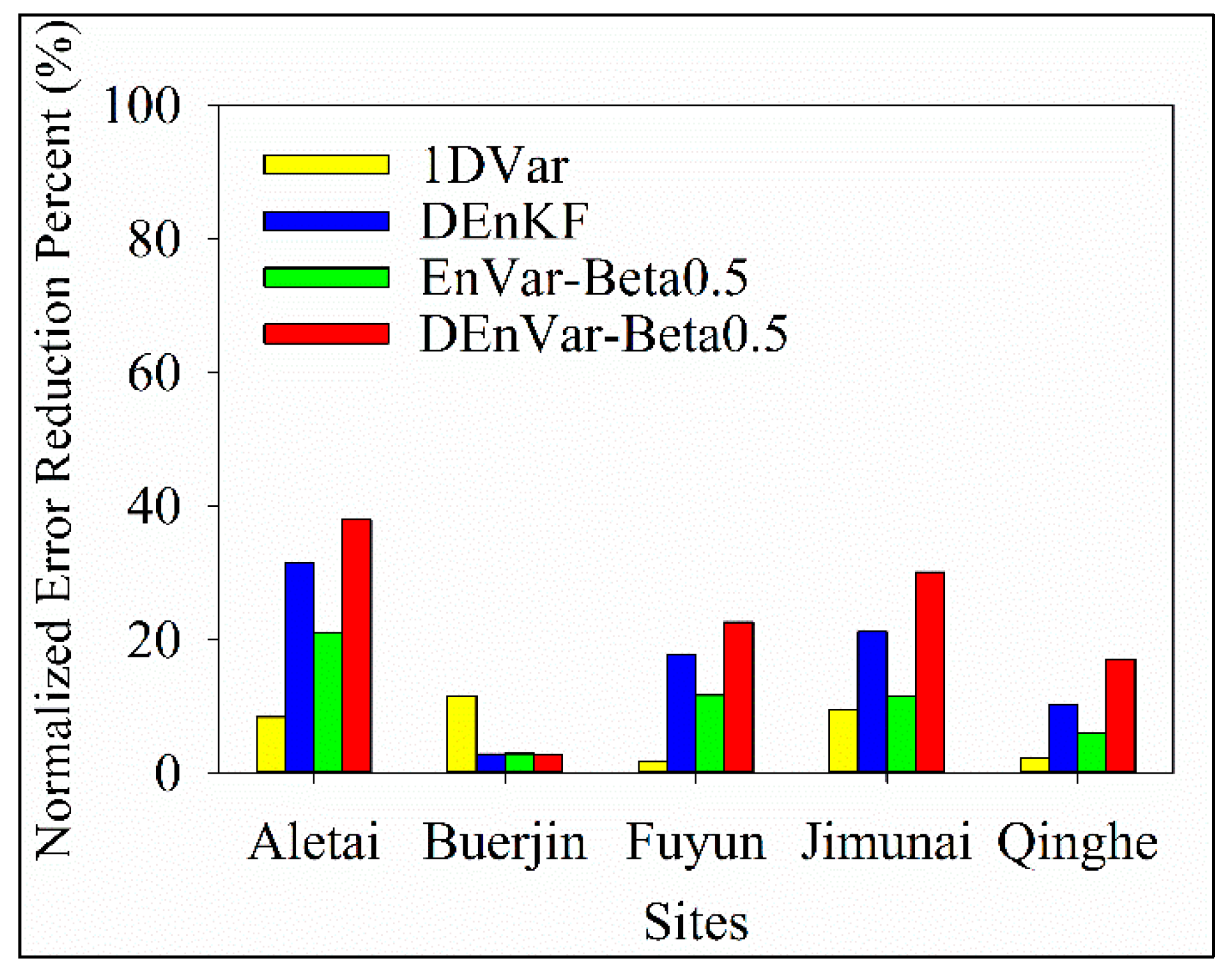
4.1. Snow Data Assimilation Using Different Methods

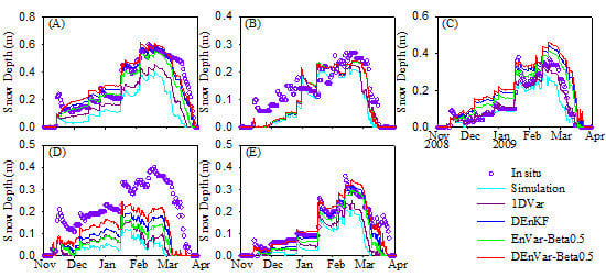
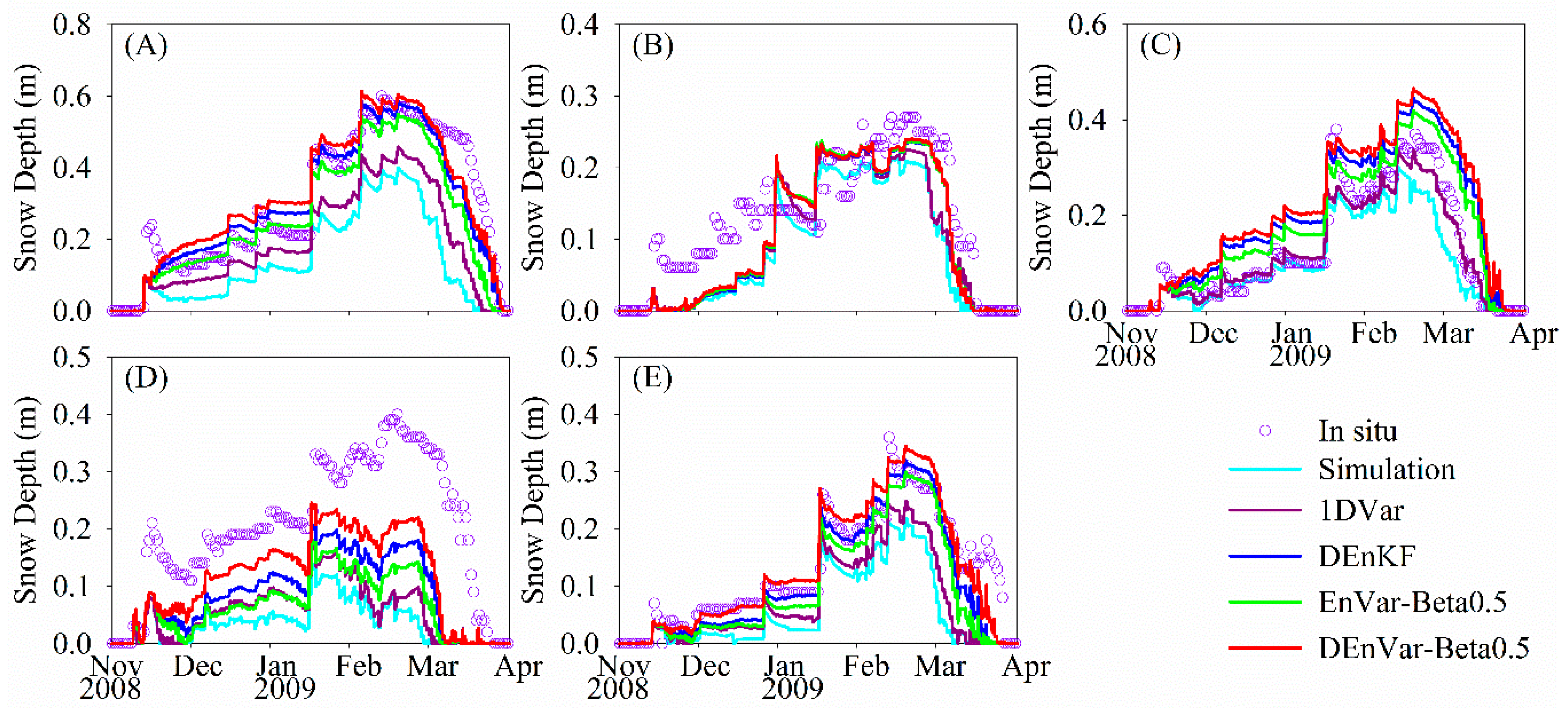
4.1.1. Comparison with In situ SD Observations

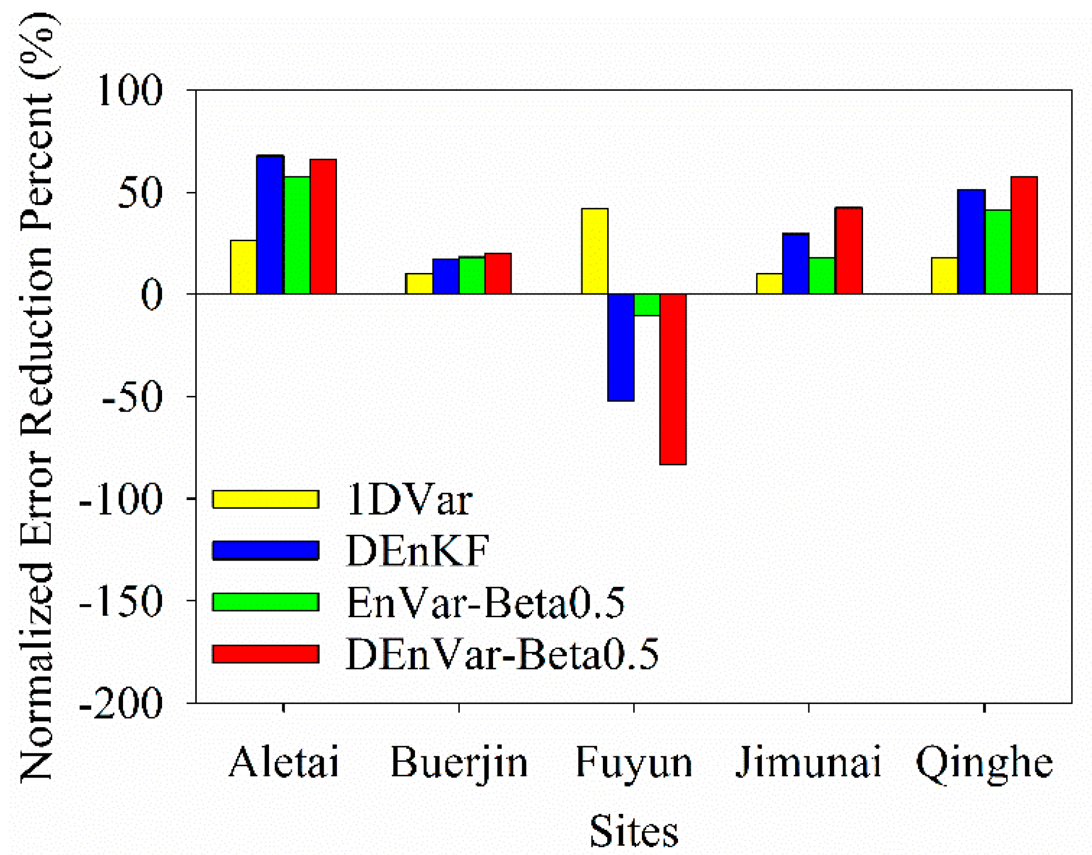
In Figure 3, the CoLM running at most sites produces late snow accumulations and early snowpack melt-offs as compared with in situ SD observations, except at the Fuyun site, partly due to underestimation of albedo and SCF in the CoLM [20]. At the Fuyun site, the CoLM simulation shows time series trends consistent with in situ SD observations during the snow accumulation period. However, there is still a large discrepancy between the CoLM-simulated SD and in situ observations during the melting period. Figure 3 shows that the four DA experiments have similar time series trends. In the experiments of DEnVar-Beta 0.5, DEnKF, and EnVar-Beta 0.5, the analyzed SD values during the snow accumulation and melting periods are elevated to a value that is very close to in situ observations at the Aletai, Buerjin, and Qinghe sites. In contrast to 1DVar experiment (see Figure 3A,B,E), these three DA experiments obtain better analysis performance. However, the opposite happened at the Fuyun site. At the Fuyun site, these three DA experiments showed overestimated peak and melting snowpack as compared with the 1DVar experiment; the 1DVar analysis tended to be similar to the in situ SD time series trend as compared with other experiments in Figure 3C. The overestimation is caused by the large positive innovation $y^o-H\left(x^b\right)$, which may be related to the predicted SCF observation underestimated by the simplified observation operator [20]. It is expected to alleviate the overestimation by improving the simplified observation operator in a method similar to the SCF parameterization scheme [10,61]. At the Jimunai site, the DEnVar-Beta0.5 experiment obtained the best analysis performance, but it tends to melt the snowpack too early and rapidly in Figure 3D. This is due to the presence of cloud cover, which accounts for the missing SCF observations in snow DA during this period [20].

Figure 3. Comparison of SD time series from in situ observations and the assimilated results from different DA experiments at the (A) Aletai, (B) Buerjin, (C) Fuyun, (D) Jimunai, and (E) Qinghe sites.

Figure 3. Comparison of SD time series from in situ observations and the assimilated results from different DA experiments at the (A) Aletai, (B) Buerjin, (C) Fuyun, (D) Jimunai, and (E) Qinghe sites.

To compare the overall difference of the four DA experiments, these results were evaluated with the indices of bias, RMSE, and temporal correlation coefficient (Correlation) in Table 3. The DEnVar-Beta 0.5 experiment with the lowest bias and RMSE and the highest correlation coefficient outperformed other DA experiments at the Buerjin, Jimunai, and Qinghe sites. Among these three sites, Qinghe tended to have the lowest errors (the bias of 0.28 cm and the RMSE of 3.91 cm) and the highest correlation coefficient of 0.95 in the DEnVar-Beta0.5 experiment. The error of the analyzed SD in the DEnVar-Beta 0.5 experiment was reduced by 57.82% (NERP of 57.82%, see Figure 4) as compared with the CoLM simulations at the Qinghe site, and the errors in other DA experiments were also reduced by 18.12%, 51.13%, and 41.42%, respectively, in Figure 4. At the Aletai site, the DEnKF experiment with a bias of −0.71 cm obtained a slightly better agreement with in situ SD observations against the DEnVar-Beta 0.5 experiment with a bias of 1.85 cm in Table 3. The improved magnitude of the DEnKF and DEnVar-Beta 0.5 experiments at the Aletai site is extended upwards to 67.93%and 66.29% respectively in Figure 4. At the Fuyun site, the correlation coefficient between the 1DVar analyzed SD and in situ SD reached 0.98, with a bias of −1.41 cm and a RMSE of 3.36 cm in Table 3. These values imply that the 1DVar experiment obtains a better agreement and smaller differences with in situ SD observations as compared with other experiments. The large positive bias in Table 3 and negative NERP values in Figure 4 show overestimation of SD during the snow accumulation and melting periods in the experiments of DEnKF, EnVar-Beta 0.5, and DEnVar-Beta 0.5, especially in the DEnVar-Beta 0.5 experiments, with the largest positive bias of 8.97 cm and negative NERP of −83.36% at the Fuyun site in Figure 4.

The bias, RMSE, correlation coefficient, and NERP values significantly improved after the assimilation of available MODIS SCF observations. On average, the four DA experiments can improve SD simulations. In particular, the DEnVar-Beta 0.5 experiment obtains the best analysis performance while the 1DVar experiment obtains the worst analysis performance. The DEnKF analysis performs as well as the analysis of DEnVar-Beta 0.5 experiment and better than that of the EnVar-Beta 0.5 experiment. Since the DEnVar-Beta 0.5 experiment integrates the analysis of DEnKF and 1DVar, the DEnVar-Beta 0.5 experiment produces more snow accumulations than the DEnKF and 1DVar experiments. This is to say, the DEnVar-Beta 0.5 experiment makes significant improvements on SD simulations, especially in the case of underestimated SD simulations.

Figure 4. The normalized error reduction percent (NEPR) of the analyzed SD in 1DVar, DEnKF, EnVar-Beta 0.5, and DEnVar-Beta 0.5 experiments. Higher NEPRs indicate an obvious improvement of snow DA.

Figure 4. The normalized error reduction percent (NEPR) of the analyzed SD in 1DVar, DEnKF, EnVar-Beta 0.5, and DEnVar-Beta 0.5 experiments. Higher NEPRs indicate an obvious improvement of snow DA.

Table 3. Summary of the analyzed SD simulation statistics in 1DVar, DEnKF, EnVar-Beta 0.5, and DEnVar-Beta 0.5 DA experiments at five sites from November 2008 to March 2009.

Index	Experiment	Aletai	Buerjin	Fuyun	Jimunai	Qinghe
Bias (m)	Simulation	−0.1759	−0.0529	−0.0398	−0.1887	−0.0811
	1DVar	−0.1221	−0.0385	−0.0141	−0.1670	−0.0630
	DEnKF	−0.0071	−0.0301	0.0714	−0.1311	−0.0218
	EnVar-Beta 0.5	−0.0453	−0.0295	0.0459	−0.1549	−0.0369
	DEnVar-Beta 0.5	0.0185	−0.0290	0.0897	−0.1011	0.0028
RMSE (m)	Simulation	0.2011	0.0689	0.0577	0.2070	0.0927
	1DVar	0.1476	0.0618	0.0336	0.1860	0.0759
	DEnKF	0.0645	0.0569	0.0878	0.1456	0.0453
	EnVar-Beta 0.5	0.0851	0.0563	0.0637	0.1696	0.0543
	DEnVar-Beta 0.5	0.0678	0.0550	0.1058	0.1192	0.0391
Correlation	Simulation	0.8391	0.8582	0.9617	0.5808	0.8560
	1DVar	0.8966	0.8599	0.9782	0.6281	0.8809
	DEnKF	0.9450	0.8820	0.9259	0.8162	0.9304
	EnVar-Beta 0.5	0.9273	0.8828	0.9422	0.7807	0.9169
	DEnVar-Beta 0.5	0.9434	0.8885	0.9146	0.8183	0.9463

Table 3. Summary of the analyzed SD simulation statistics in 1DVar, DEnKF, EnVar-Beta 0.5, and DEnVar-Beta 0.5 DA experiments at five sites from November 2008 to March 2009.

Index	Experiment	Aletai	Buerjin	Fuyun	Jimunai	Qinghe
Bias (m)	Simulation	−0.1759	−0.0529	−0.0398	−0.1887	−0.0811
	1DVar	−0.1221	−0.0385	−0.0141	−0.1670	−0.0630
	DEnKF	−0.0071	−0.0301	0.0714	−0.1311	−0.0218
	EnVar-Beta 0.5	−0.0453	−0.0295	0.0459	−0.1549	−0.0369
	DEnVar-Beta 0.5	0.0185	−0.0290	0.0897	−0.1011	0.0028
RMSE (m)	Simulation	0.2011	0.0689	0.0577	0.2070	0.0927
	1DVar	0.1476	0.0618	0.0336	0.1860	0.0759
	DEnKF	0.0645	0.0569	0.0878	0.1456	0.0453
	EnVar-Beta 0.5	0.0851	0.0563	0.0637	0.1696	0.0543
	DEnVar-Beta 0.5	0.0678	0.0550	0.1058	0.1192	0.0391
Correlation	Simulation	0.8391	0.8582	0.9617	0.5808	0.8560
	1DVar	0.8966	0.8599	0.9782	0.6281	0.8809
	DEnKF	0.9450	0.8820	0.9259	0.8162	0.9304
	EnVar-Beta 0.5	0.9273	0.8828	0.9422	0.7807	0.9169
	DEnVar-Beta 0.5	0.9434	0.8885	0.9146	0.8183	0.9463

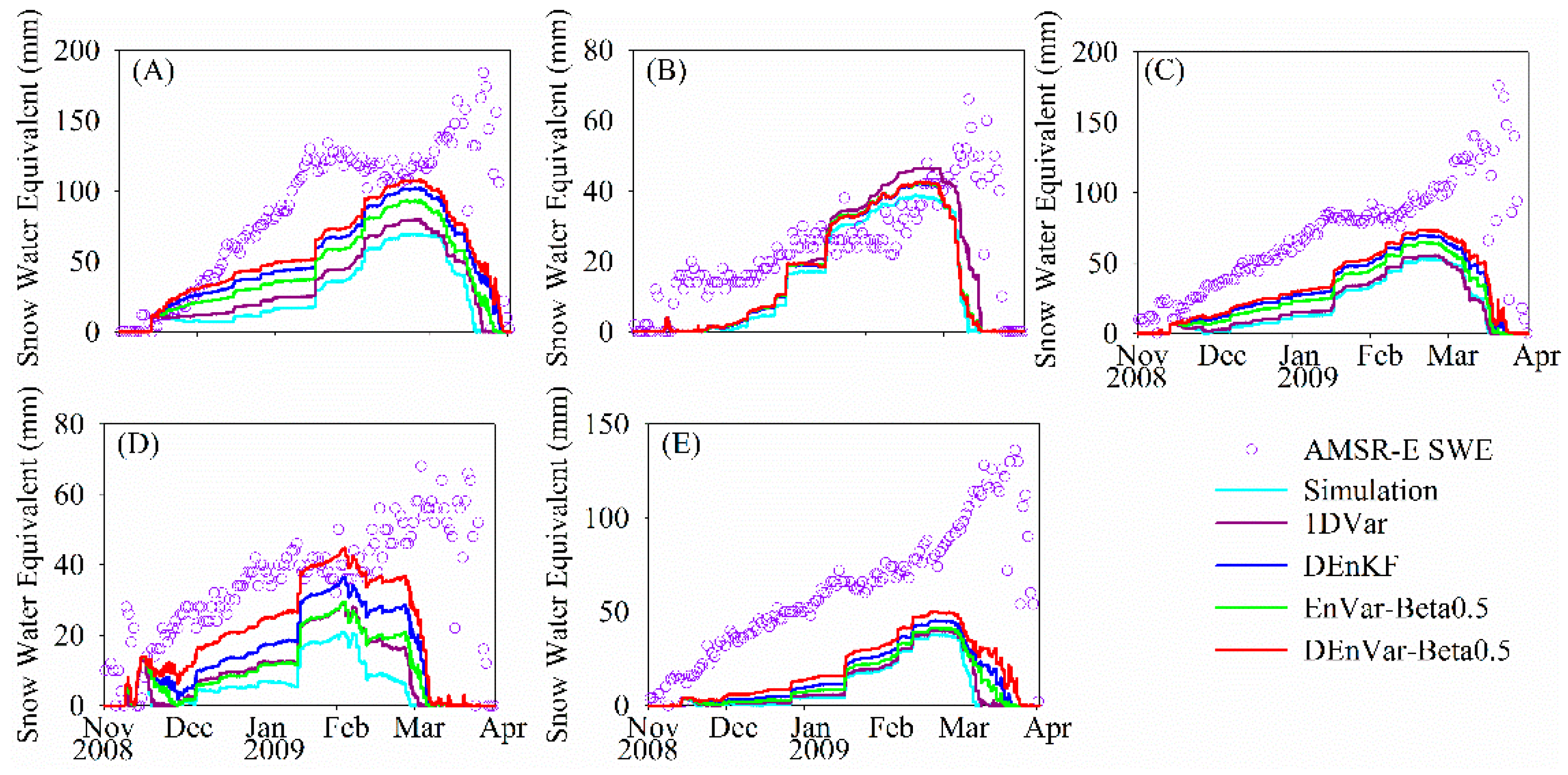
4.1.2. Comparison with AMSR-E SWE Observations

The SWE state is updated with the error covariance between the SD and SWE states using a similar algorithm of the SD update.

In Figure 5, the four DA experiments significantly improve the SWE simulations at all sites, and all DA experiments show similar SWE time series trends. However, the analyzed SWEs in these DA experiments are still underestimated during the snow accumulation and melting periods in Figure 5. From November to late February, when perhaps the snow is dry, the AMSR-E-retrieved SWE has fewer errors introduced by liquid water content [62]. These snow DA experiments show better agreement with the AMSR-E SWE observations during this period than during the melting period of March in Figure 5.

On the whole, the DEnVar-Beta 0.5 experiment obtained better analysis performance than other DA experiments at the Aletai, Fuyun, Jimunai, and Qinghe sites in Figure 5, with the lowest bias and RMSE and highest correlation coefficient values in Table 4. At the Aletai site, the bias between the analyzed SWE in the DEnVar-Beta 0.5 experiment and the AMSR-E SWE was reduced from −60.69 mm (the bias of the CoLM simulations) to −30.74 mm, and the RMSE was reduced from 72.17 mm to 44.78 mm. The DEnVar-Beta 0.5 experiment tended to have the largest improved magnitude of SWE at the Aletai site and the improved magnitude reached 37.95% in Figure 6. As compared with the EnVar-Beta 0.5 experiment, the DEnKF experiment showed analysis results similar to that of the DEnVar-Beta 0.5 experiment, and achieved a slightly better agreement with the AMSR-E SWE observations. The EnVar-Beta 0.5 experiment with a NERP of 21% outperformed the 1DVar experiment with a NERP of 8.45% in Figure 6, conversely, at the Buerjin site. At the Buerjin site, the 1DVar experiment offered better improvement than other DA experiments. As compared with the CoLM simulations, the SWE simulations of the 1DVar has obtained an 11.6% improved magnitude, while the largest improved magnitude among the DEnKF, EnVar-Beta0.5, and DEnVar-Beta 0.5 experiments was only 2.92%, in the EnVar-Beta 0.5 experiment in Figure 6.

Figure 5. Comparison of the SWE time series from AMSR-E retrieved SWE and the assimilated results from different DA experiments at the (A) Aletai, (B) Buerjin, (C) Fuyun, (D) Jimunai, and (E) Qinghe sites.

Figure 5. Comparison of the SWE time series from AMSR-E retrieved SWE and the assimilated results from different DA experiments at the (A) Aletai, (B) Buerjin, (C) Fuyun, (D) Jimunai, and (E) Qinghe sites.

Figure 6. Analysis of SWE state. Cf. Figure 4.

Figure 6. Analysis of SWE state. Cf. Figure 4.

Table 4. Summary of the analyzed SWE statistics. Cf. Table 3.

Index	Experiment	Aletai	Buerjin	Fuyun	Jimunai	Qinghe
Bias (mm)	Simulation	−60.6890	−10.7972	−51.1207	−30.8255	−51.9142
	1DVar	−54.1836	−6.5794	−49.6650	−26.8484	−50.5498
	DEnKF	−36.1520	−9.1861	−38.9930	−21.8406	−46.2824
	EnVar-Beta 0.5	−43.9760	−8.9642	−43.0146	−26.2549	−48.6462
	DEnVar-Beta 0.5	−30.7429	−8.9699	−36.0278	−16.3484	−42.4852
	Simulation	72.1651	19.5319	59.9968	34.2670	60.4474
RMSE (mm)	1DVar	66.0648	17.2661	58.9658	30.9795	59.0669
	DEnKF	49.4169	18.9730	49.2967	27.0125	54.2969
	EnVar-Beta 0.5	57.0112	18.9613	52.9896	30.3120	56.7938
	DEnVar-Beta 0.5	44.7758	18.9999	46.4075	23.9441	50.1661
Correlation	Simulation	0.5940	0.4602	0.5499	0.1439	0.3393
	1DVar	0.6361	0.5819	0.5339	0.2447	0.3715
	DEnKF	0.7420	0.4782	0.6021	0.3305	0.5072
	EnVar-Beta 0.5	0.6809	0.4769	0.5712	0.2767	0.4538
	DEnVar-Beta 0.5	0.7657	0.4740	0.6339	0.3495	0.5936

Table 4. Summary of the analyzed SWE statistics. Cf. Table 3.

Index	Experiment	Aletai	Buerjin	Fuyun	Jimunai	Qinghe
Bias (mm)	Simulation	−60.6890	−10.7972	−51.1207	−30.8255	−51.9142
	1DVar	−54.1836	−6.5794	−49.6650	−26.8484	−50.5498
	DEnKF	−36.1520	−9.1861	−38.9930	−21.8406	−46.2824
	EnVar-Beta 0.5	−43.9760	−8.9642	−43.0146	−26.2549	−48.6462
	DEnVar-Beta 0.5	−30.7429	−8.9699	−36.0278	−16.3484	−42.4852
	Simulation	72.1651	19.5319	59.9968	34.2670	60.4474
RMSE (mm)	1DVar	66.0648	17.2661	58.9658	30.9795	59.0669
	DEnKF	49.4169	18.9730	49.2967	27.0125	54.2969
	EnVar-Beta 0.5	57.0112	18.9613	52.9896	30.3120	56.7938
	DEnVar-Beta 0.5	44.7758	18.9999	46.4075	23.9441	50.1661
Correlation	Simulation	0.5940	0.4602	0.5499	0.1439	0.3393
	1DVar	0.6361	0.5819	0.5339	0.2447	0.3715
	DEnKF	0.7420	0.4782	0.6021	0.3305	0.5072
	EnVar-Beta 0.5	0.6809	0.4769	0.5712	0.2767	0.4538
	DEnVar-Beta 0.5	0.7657	0.4740	0.6339	0.3495	0.5936

Although the analyzed SWE values during the snow accumulation and melting periods were improved, a large discrepancy still exists between the analyzed SWE and the AMSR-E SWE. That resulted partially from the imprecise covariance between SD and SWE states. An improved extent of the SWE state is determined by innovation $d=y^o-H\left(x^b\right)$ and Kalman gain concerning the covariance between SD and SWE states. The covariance is underestimated with an inaccurate covariance. The underestimated covariance may decrease the Kalman gain, and further lead to a sub-optimal assimilation.

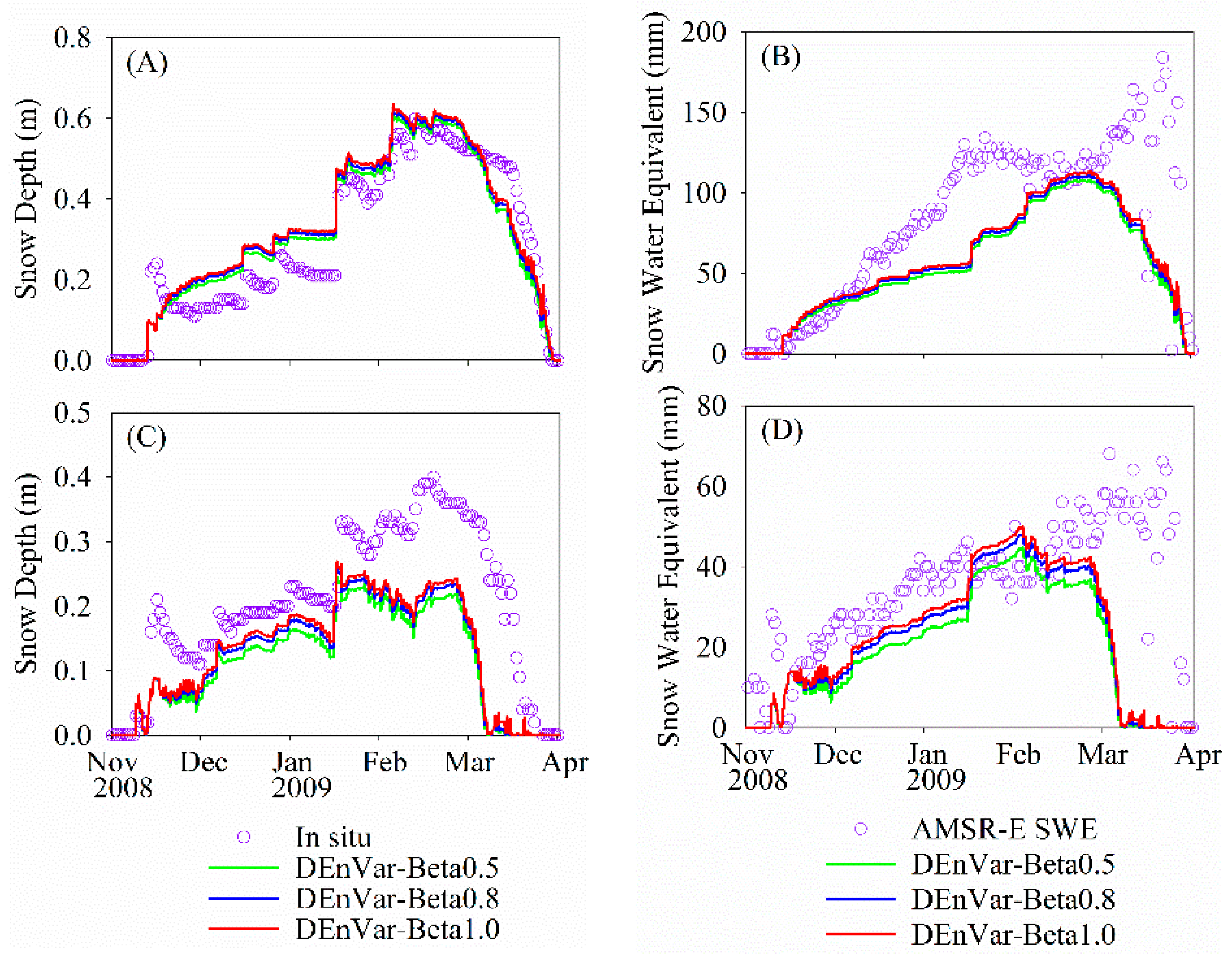
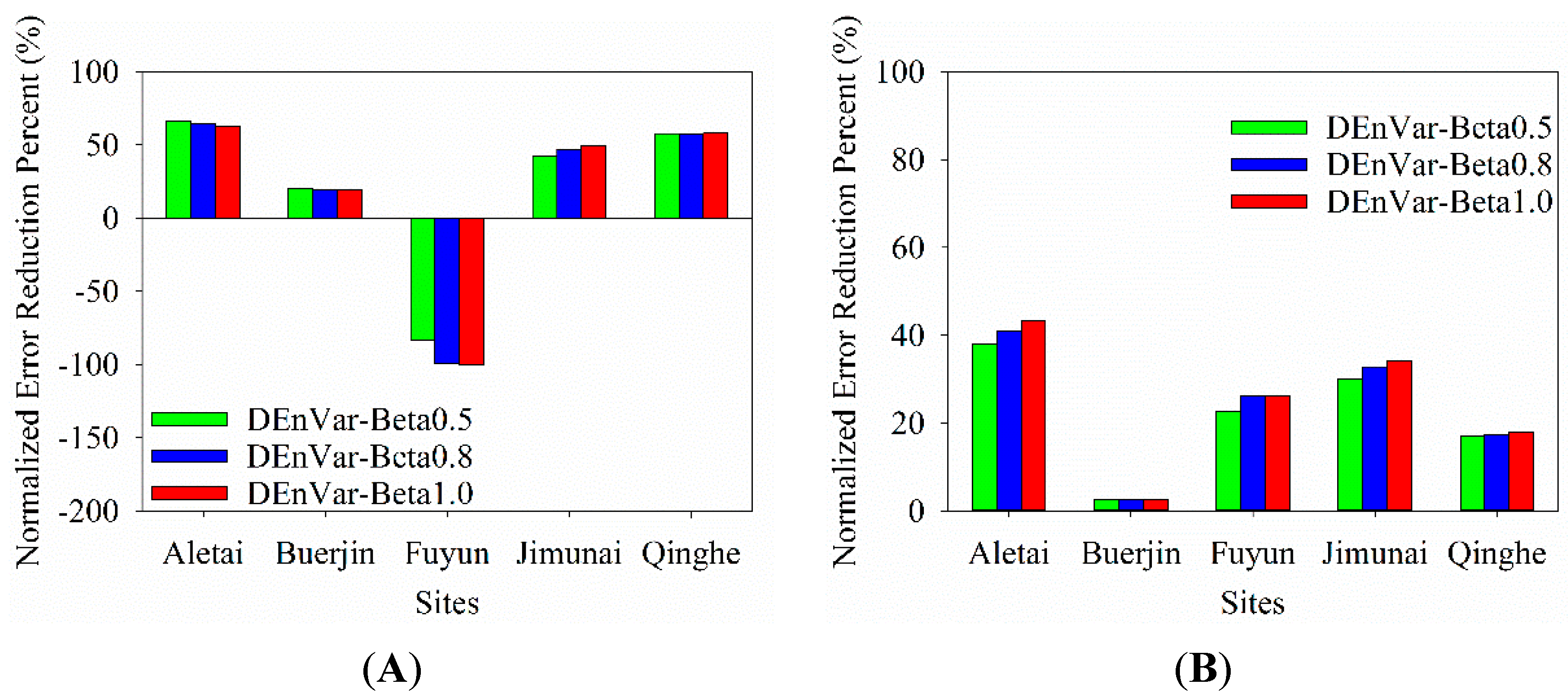
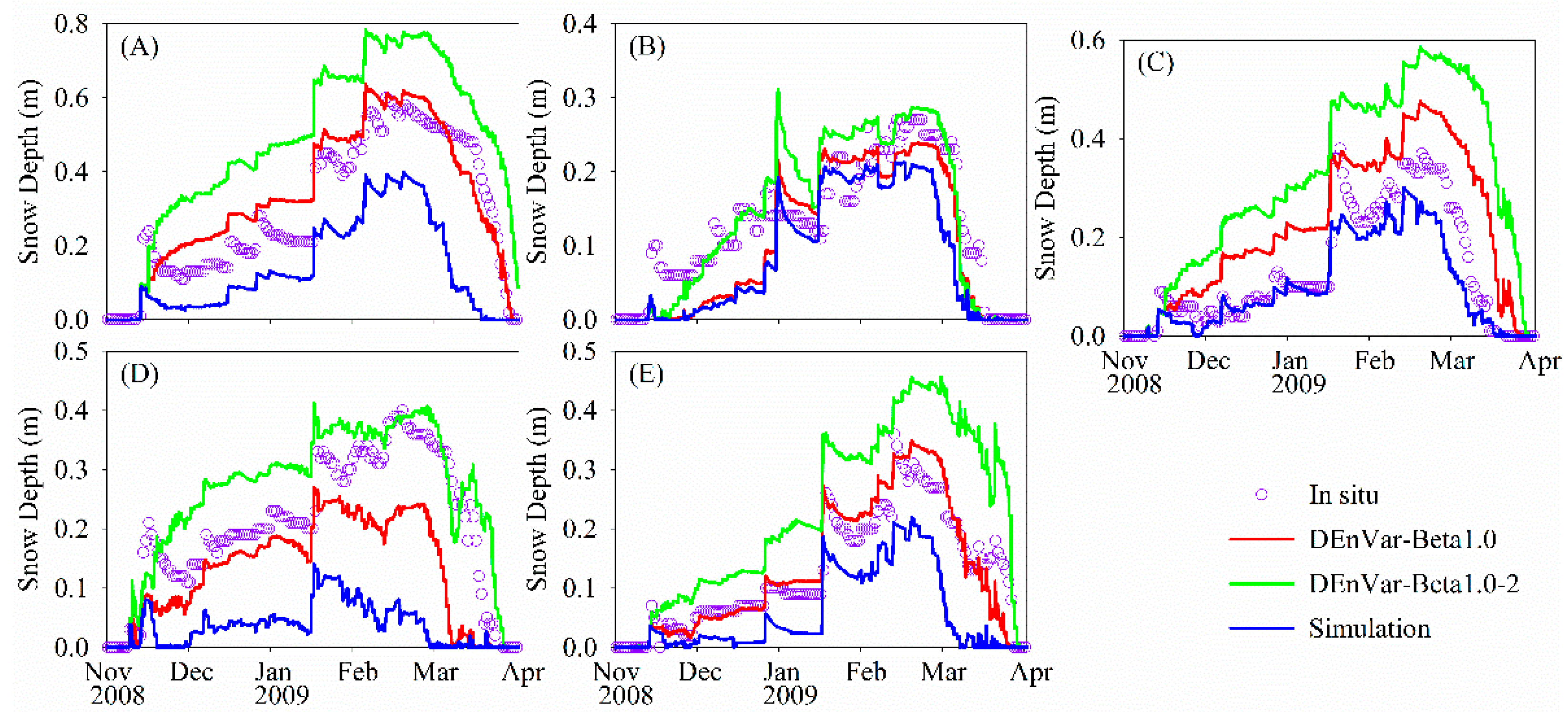
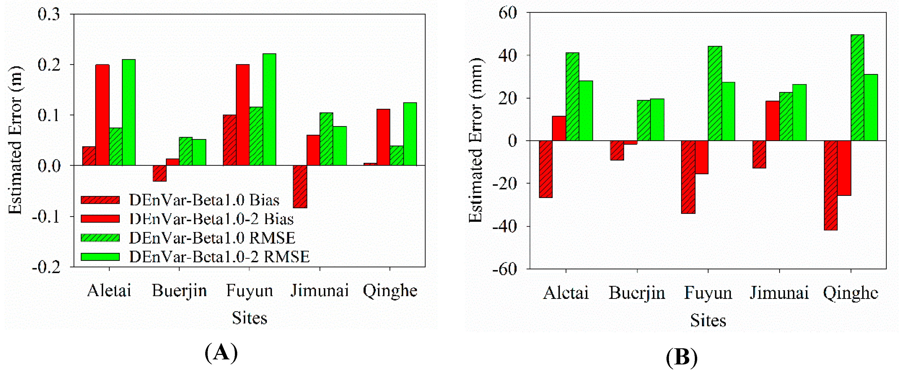
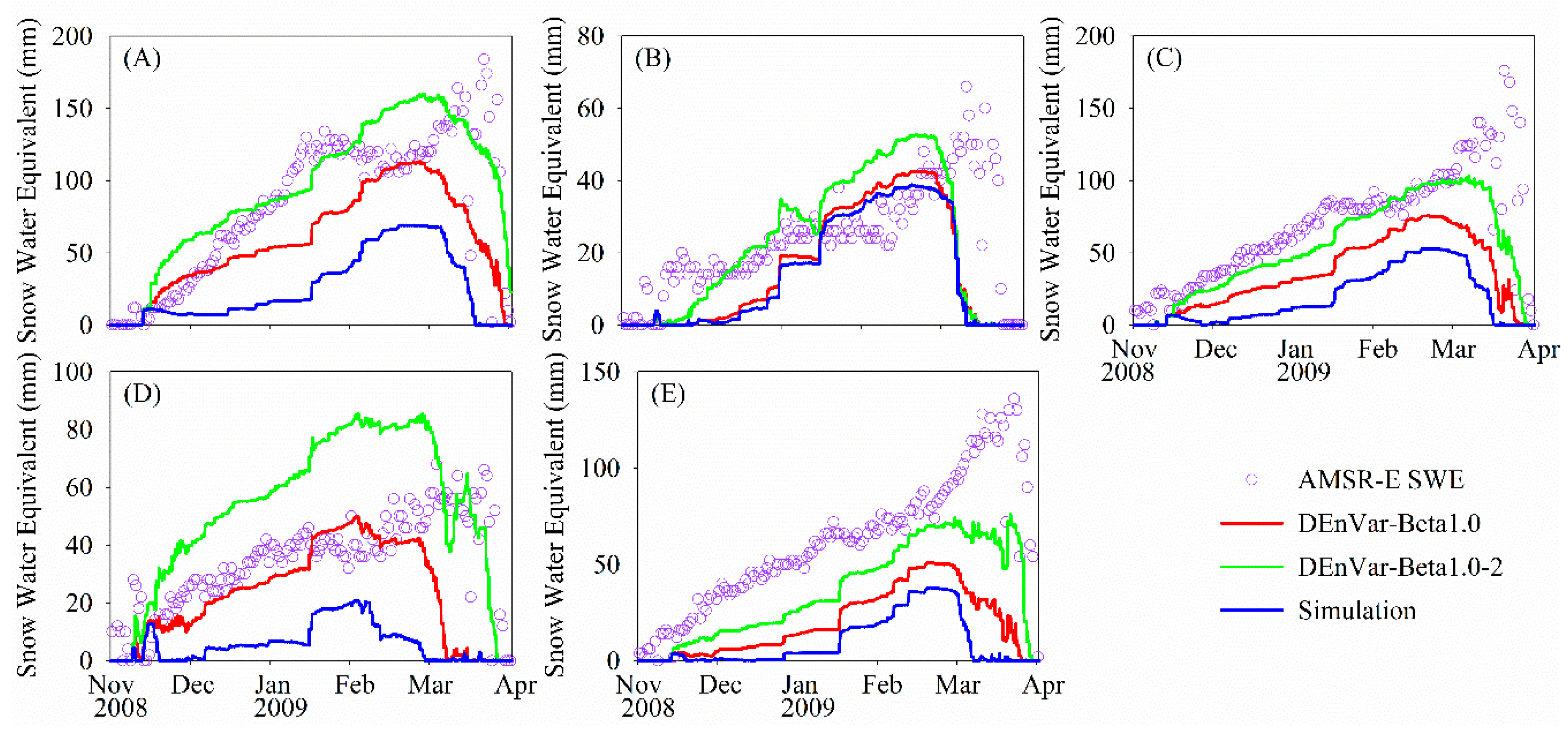
4.2. Sensitivity to Weighting Coefficients

Here we performed the sensitivity test of the weighting coefficient β to the proposed DEnVar method. The weighting coefficient β, as given in Equation (11), controls the respective weights of the static NMC and ensemble-based analysis error covariances. The weighting coefficient is set to 0.8 in the DEnVar. This explains that 20% of the covariance comes from the static NMC estimate and 80% from the ensemble error statistic, as described in the DEnVar-Beta 0.8 experiment. The weighting coefficient was set to 1. This explains that the hybrid error covariance only contains the ensemble-based analysis error covariance (as in the DEnVar-Beta 1.0 experiment).

Figure 7 shows the time series of the CoLM snow states from the DEnVar experiment, with β of 0.5 in the DEnVar-Beta 0.5 experiment, 0.8 in the DEnVar-Beta 0.8 experiment, and 1.0 in the DEnVar-Beta 1.0 experiment at the Aletai and Jimunai sites. The time series graphics at other sites are not shown given their similar analysis performance. In Figure 7, the three DA experiments show similar time series trends; the DEnVar-Beta 1.0 experiment obtained a slightly closer fit to snow observations than the DEnVar-Beta 0.5 and DEnVar-Beta 0.8 experiments. For the SD state, the three DA experiments have similar NERP values in Figure 8A, while the DEnVar-Beta 1.0 experiment has lower NERP values at the Aletai, Buerjin, and Fuyun sites, and higher NERP values at the Jimunai and Qinghe sites than in the other DA experiments. In addition, for the SWE state, the DEnVar-Beta 1.0 experiment with slightly higher NERP values achieved a slightly better analysis performance than the DEnVar-Beta 0.5 and DEnVar-Beta 0.8 experiments at all sites (Figure 8B). Therefore, it is concluded that the proposed DEnVar method is not highly sensitive to the weighting coefficient β. However, it prefers to give greater weight to the ensemble-based analysis error covariance since the DEnVar experiment with a greater weighting coefficient produces more snow accumulations and achieves better correlation with snow observations, especially in the case of SD- and SWE-underestimated simulations.

Figure 7. The time series comparison of CoLM snow states (Left: SD, Right: SWE) from snow observations and the assimilated results in DEnVar-Beta 0.5, DEnVar-Beta 0.8, and DEnVar-Beta 1.0 sensitivity tests at the Aletai (A,B) and Jimunai sites (C,D).

Figure 7. The time series comparison of CoLM snow states (Left: SD, Right: SWE) from snow observations and the assimilated results in DEnVar-Beta 0.5, DEnVar-Beta 0.8, and DEnVar-Beta 1.0 sensitivity tests at the Aletai (A,B) and Jimunai sites (C,D).

Figure 8. The NEPR of the analyzed SD (A) and SWE (B) in the DEnVar-Beta 0.5, DEnVar-Beta 0.8, and DEnVar-Beta 1.0 sensitivity tests.

Figure 8. The NEPR of the analyzed SD (A) and SWE (B) in the DEnVar-Beta 0.5, DEnVar-Beta 0.8, and DEnVar-Beta 1.0 sensitivity tests.

4.3. Sensitivity to Observation Error

Given that MODIS SCF products have approximately 10% error [54,63], some previous studies have assigned a 10% SCF observation error to MODIS SCF DA [16,17]. To identify the influence of this 10% SCF observation error on the proposed DEnVar DA method, a sensitivity test extending the DEnVar-Beta 1.0 experiment, a DEnVar-Beta 1.0–2 experiment, was performed.

In Figure 9, the DEnVar-Beta 1.0–2 experiment showed an overestimated peak snowpack as compared with the DEnVar-Beta 1.0 experiment, which produced early snow accumulations and late snowpack melt-offs at all sites except for Buerjin. The DEnVar-Beta 1.0–2 experiment tended to overestimate the SD simulations at all sites, leading to large bias and RMSE values in Figure 10A. The Fuyun site has the largest bias of 20.06 cm and the largest RMSE of 22.10 cm. The lowest bias of 1.33 cm and RMSE of 5.19 cm occurred at the Buerjin site (Figure 10A).

Figure 9. The SD time series of in situ SD observations and the analyzed SD in the DEnVar-Beta 1.0 and DEnVar-Beta 1.0–2 sensitivity tests at the (A) Aletai, (B) Buerjin, (C) Fuyun, (D) Jimunai, and (E) Qinghe sites. The observation standard errors (σ_obs) at five sites in the DEnVar-Beta 1.0 experiment are given in Table 1. The DEnVar-Beta 1.0–2 experiment is the same as the DEnVar-Beta 1.0 experiment, but the MODIS SCF observation error is set to 10%.

Figure 9. The SD time series of in situ SD observations and the analyzed SD in the DEnVar-Beta 1.0 and DEnVar-Beta 1.0–2 sensitivity tests at the (A) Aletai, (B) Buerjin, (C) Fuyun, (D) Jimunai, and (E) Qinghe sites. The observation standard errors (σ_obs) at five sites in the DEnVar-Beta 1.0 experiment are given in Table 1. The DEnVar-Beta 1.0–2 experiment is the same as the DEnVar-Beta 1.0 experiment, but the MODIS SCF observation error is set to 10%.

Figure 10. The bias and RMSE of the analyzed SD (A) and SWE (B) in DEnVar-Beta 1.0–2 experiment with the MODIS SCF observation error of 10%.

Figure 10. The bias and RMSE of the analyzed SD (A) and SWE (B) in DEnVar-Beta 1.0–2 experiment with the MODIS SCF observation error of 10%.

Figure 11 shows that the analyzed SWE values in the peak and melting stages were greatly increased. This led to overestimation of the SWE simulations at the Aletai and Jimunai sites, with positive biases of 11.39 mm and 18.99 mm, respectively (Figure 10B). Although the analyzed SWE is still underestimated at the Fuyun and Qinghe sites (as seen in the negative bias in Figure 10B), the time series trend from the DEnVar-Beta 1.0–2 experiment was closer to that of the AMSR-E-retrieved SWE observations than that from the DEnVar-Beta 1.0 experiment in Figure 11.

Figure 11. Graphical representation of the SWE state. Cf. Figure 9.

Figure 11. Graphical representation of the SWE state. Cf. Figure 9.

On the whole, large changes in the SD and SWE states were produced by the DEnVar-Beta 1.0–2 experiment, with a 10% SCF observation error. In sum, the proposed DEnVar method is highly sensitive to observation error. Moreover, a reasonable MODIS SCF observation error is quite important for snow DA. A triple collocation technique [64] may be used to estimate the MODIS SCF observation error under the assumption that the three snow-related datasets are independent of each other.

5. Conclusions

In this study, four different data assimilation (DA) experiments assimilating MODIS SCF observations into the CoLM were performed using ensemble-based, variational, and hybrid methods, DEnKF, 1DVar, EnVar (a hybrid ensemble-variational DA system), and DEnVar (DEnKF-1DVar). EnVar and DEnVar are coupled DA methods, which are comparable to the method of Zhang et al. [36] and couple 1DVar and DEnKF methods. Unlike EnVar, the DEnVar method needs a two-step process. That is, the analysis ensemble mean and the analysis error covariance of DEnKF are introduced into the 1DVar hybrid cost function, and the analysis mean of DEnKF is replaced by the 1DVar analysis.

DA experiments were performed at five sites in the Altay region of China from November 2008 to March 2009. The analyzed SD and SWE were validated against in situ SD and AMSR-E SWE observations. Our results indicate that some improvements in the four DA experiments occurred at most sites when the available MODIS SCF is assimilated. It was shown that, with the same observation errors, the 1DVar of static NMC-based background error covariance performed worse than other DA methods of ensemble-based background error covariance. This indicates that the static NMC-based background error covariance magnitude from 1DVar is less than the ensemble-based background error covariance from the DEnKF. A possible reason is that a larger analysis error covariance $P_{en}^a=\left(I-KH\right)P_{en}^b+\raisebox{1ex}{$1$}\!\left/ \!\raisebox{-1ex}{$4$}\right.KH{P}_{en}^b{H}^T{K}^T$ of the DEnKF method is calculated by the equations $P_{en}^a=\overline{A^a{\left(A^a\right)}^T}$ and $A^a=A^b-\raisebox{1ex}{$1$}\!\left/ \!\raisebox{-1ex}{$2$}\right.KH{A}^b$. This analysis error covariance explains that the DEnKF can avoid underestimating the analysis error covariance [41]. As compared with the stochastic EnKF, an additional term $\raisebox{1ex}{$1$}\!\left/ \!\raisebox{-1ex}{$4$}\right.KH{P}_{en}^b{H}^T{K}^T$ in the DEnKF is interpreted as an inherent covariance inflation, which can effectively maintain the ensemble spread and avoid filter divergence. Furthermore, the DEnKF without observation perturbations does not introduce extra observation perturbation errors, which may render the filter sub-optimal [40]. The analysis error covariance $P_{en}^a$ and ensemble mean ${\overline{x}}_{en}^a$ of DEnKF are used in the hybrid 1DVar cost function (DEnVar-Beta 0.5). The 1DVar analysis in DEnVar-Beta 0.5 experiment is better than that in the EnVar-Beta 0.5 experiment, which uses the forecast error covariance $P_{en}^b$ and ensemble mean ${\overline{x}}_{en}^b$. As a result, our hybrid DEnVar method obtains better analysis performance than the EnVar method of Zhang et al. [36]. The analysis performance of the two-step DEnVar method is better than that of the DEnKF method.

Although our hybrid DA method can improve the simulations of SD and SWE to some extent, large errors can still be found in snow simulations of the CoLM. The large errors may be partly due to the scale mismatch between the CoLM model and input datasets. In practice, the atmospheric forcing data with a 0.1° spatial resolution is effectively implemented to drive the CoLM with a 0.01° spatial resolution in simulations and assimilations of SD and SWE. However, this atmospheric forcing data at a larger scale may introduce some errors leading to a bias in simulations of SD and SWE. It is due to this that atmospheric forcing data may not satisfy the requirements of simulations and assimilations on the CoLM’s scale, as well as the assimilated MODIS SCF with a 500 m spatial resolution. Furthermore, to be consistent with the CoLM’s scale, the AMSR-E SWE data is downscaled to a spatial resolution of 0.01° using a nearest neighbor resampling. The value of the scaled SWE data does not differ from the original SWE data value with a 25 km spatial resolution. Thus, the scaled SWE data used to estimate the observation errors and validate the assimilated results may also have introduced some errors into our DA experiments.

Lastly, we tested the sensitivity of the weighting coefficient of hybrid background error covariance and the SCF observation error to the DEnVar method, respectively. It is found that the proposed DEnVar method is slightly sensitive to the weighting coefficient and is highly sensitive to observation errors. The DEnVar-Beta 1.0 experiment with the ensemble-based analysis error covariance $P_{en}^a$ obtains better analysis performance than the DEnVar-Beta 0.5 and DEnVar-Beta 0.8 experiments with the hybrid error covariance, because the element values of background error covariance calculated with the hybrid error covariance are decreased in the 1DVar cost function. It is thus feasible to use only the ensemble-based error covariance from the DEnKF in the hybrid DA system.

References

1. Simic, A.; Fernandes, R.; Brown, R.; Romanov, P.; Park, W. Validation of vegetation, MODIS, and GOES+ SSM/I snow-cover products over canada based on surface snow depth observations. Hydrol. Process. 2004, 18, 1089–1104. [Google Scholar] [CrossRef]
2. Evaluation of Surface Albedo and Snow Cover in AR4 Coupled Climate Models. Available online: http://onlinelibrary.wiley.com/doi/10.1029/2005JD006473/citedby (accessed on 16 August 2006).
3. Frei, A.; Tedesco, M.; Lee, S.; Foster, J.; Hall, D.K.; Kelly, R.; Robinson, D.A. A review of global satellite-derived snow products. Adv. Space Resour. 2012, 50, 1007–1029. [Google Scholar] [CrossRef]
4. Evaluation of an Improved Intermediate Complexity Snow Scheme in the Orchidee Land Surface Model. Available online: http://onlinelibrary.wiley.com/doi/10.1002/jgrd.50395/abstract (accessed on 27 June 2013).
5. Scanning Multichannel Microwave Radiometer Snow Water equivalent Assimilation. Available online: http://onlinelibrary.wiley.com/doi/10.1029/2006JD007209/abstract (accessed on 16 April 2007).
6. Liang, T.G.; Zhang, X.T.; Xie, H.J.; Wu, C.X.; Feng, Q.S.; Huang, X.D.; Chen, Q.G. Toward improved daily snow cover mapping with advanced combination of MODIS and AMSR-E measurements. Remote Sens. Environ. 2008, 112, 3750–3761. [Google Scholar] [CrossRef]
7. Dai, L.; Che, T.; Wang, J.; Zhang, P. Snow depth and snow water equivalent estimation from AMSR-E data based on a priori snow characteristics in Xinjiang, China. Remote Sens. Environ. 2012, 127, 14–29. [Google Scholar] [CrossRef]
8. Liang, T.G.; Liu, X.Y.; Wu, C.X.; Guo, Z.G.; Huang, X.D. An evaluation approach for snow disasters in the pastoral areas of northern Xinjiang, China. New Zeal. J. Agr. Res. 2007, 50, 369–380. [Google Scholar] [CrossRef]
9. Liang, T.G.; Wu, C.X.; Chen, Q.G.; Xu, Z.B. Snow classification and monitoring models in the pastoral areas of the northern Xinjiang. J. Glaciol. Geocryol. 2004, 26, 160–165. [Google Scholar]
10. Zaitchik, B.F.; Rodell, M. Forward-looking assimilation of MODIS-derived snow-covered area into a land surface model. J. Hydrometeorol. 2009, 10, 130–148. [Google Scholar] [CrossRef]
11. Rodell, M.; Houser, P.R. Updating a land surface model with MODIS-derived snow cover. J. Hydrometeorol. 2004, 5, 1064–1075. [Google Scholar] [CrossRef]
12. Liu, Y.; Peters-Lidard, C.D.; Kumar, S.; Foster, J.L.; Shaw, M.; Tian, Y.; Fall, G.M. Assimilating satellite-based snow depth and snow cover products for improving snow predictions in Alaska. Adv. Water Resour. 2013, 54, 208–227. [Google Scholar] [CrossRef]
13. Fletcher, S.J.; Liston, G.E.; Hiemstra, C.A.; Miller, S.D. Assimilating MODIS and AMSR-E snow observations in a snow evolution model. J. Hydrometeorol. 2012, 13, 1475–1492. [Google Scholar] [CrossRef]
14. Kumar, S.V.; Reichle, R.H.; Peters-Lidard, C.D.; Koster, R.D.; Zhan, X.W.; Crow, W.T.; Eylander, J.B.; Houser, P.R. A land surface data assimilation framework using the land information system: Description and applications. Adv. Water Resour. 2008, 31, 1419–1432. [Google Scholar] [CrossRef]
15. De Lannoy, G.J.M.; Reichle, R.H.; Arsenault, K.R.; Houser, P.R.; Kumar, S.; Verhoest, N.E.C.; Pauwels, V.R.N. Multiscale assimilation of Advanced Microwave Scanning Radiometer-EOS snow water equivalent and Moderate Resolution Imaging Spectroradiometer snow cover fraction observations in northern Colorado. Water Resour. Res. 2012, 48. [Google Scholar] [CrossRef] [Green Version]
16. Andreadis, K.M.; Lettenmaier, D.P. Assimilating remotely sensed snow observations into a macroscale hydrology model. Adv. Water Resour. 2006, 29, 872–886. [Google Scholar]
17. Su, H.; Yang, Z.-L.; Niu, G.-Y.; Dickinson, R.E. Enhancing the estimation of continental-scale snow water equivalent by assimilating MODIS snow cover with the ensemble kalman filter. J. Geophys. Res. 2008, 113. [Google Scholar] [CrossRef]
18. Slater, A.G.; Clark, M.P. Snow data assimilation via an ensemble Kalman filter. J. Hydrometeorol. 2006, 7, 478–493. [Google Scholar] [CrossRef]
19. Zhang, Y.F.; Hoar, T.J.; Yang, Z.L.; Anderson, J.L.; Toure, A.M.; Rodell, M. Assimilation of MODIS snow cover through the data assimilation research testbed and the community land model version 4. J. Geophys. Res. Atmos. 2014, 119, 7091–7103. [Google Scholar]
20. Assimilating MODIS-Based Albedo and Snow Cover Fraction into the Common Land Model to Improve Snow Depth Simulation with Direct Insertion and Deterministic Ensemble Kalman Filter Methods. Available online: http://www.readcube.com/articles/10.1002/2014JD022012 (accessed on 27 September 2014).
21. Kolberg, S.; Rue, H.; Gottschalk, L. A bayesian spatial assimilation scheme for snow coverage observations in a gridded snow model. Hydrol. Earth Syst. Sci. 2006, 10, 369–381. [Google Scholar] [CrossRef] [Green Version]
22. Leisenring, M.; Moradkhani, H. Snow water equivalent prediction using bayesian data assimilation methods. Stoch. Environ. Res. Risk Assess. 2010, 25, 253–270. [Google Scholar] [CrossRef]
23. Thirel, G.; Salamon, P.; Burek, P.; Kalas, M. Assimilation of MODIS snow cover area data in a distributed hydrological model using the particle filter. Remote Sens. 2013, 5, 5825–5850. [Google Scholar] [CrossRef]
24. Clark, M.P.; Slater, A.G.; Barrett, A.P.; Hay, L.E.; McCabe, G.J.; Rajagopalan, B.; Leavesley, G.H. Assimilation of snow covered area information into hydrologic and land-surface models. Adv. Water Resour. 2006, 29, 1209–1221. [Google Scholar] [CrossRef]
25. Impacts of Snow Cover Fraction Data Assimilation on Modeled Energy and Moisture Budgets. Available online: http://www.prhouser.com/houser_files/jgrd50542.pdf (accessed on 27 July 2013).
26. Forman, B.A.; Reichle, R.H.; Rodell, M. Assimilation of terrestrial water storage from grace in a snow-dominated basin. Water Resour. Res. 2012, 48. [Google Scholar] [CrossRef]
27. Che, T.; Li, X.; Jin, R.; Huang, C. Assimilating passive microwave remote sensing data into a land surface model to improve the estimation of snow depth. Remote Sens. Environ. 2014, 143, 54–63. [Google Scholar] [CrossRef]
28. Hamill, T.M.; Snyder, C. A hybrid ensemble kalman filter-3D variational analysis scheme. Mon. Weather Rev. 2000, 128, 2905–2919. [Google Scholar] [CrossRef]
29. Lorenc, A.C. The potential of the ensemble Kalman filter for NWP—A comparison with 4D-Var. Q. J. Roy. Meteor. Soc. 2003, 129, 3183–3203. [Google Scholar] [CrossRef]
30. Wang, X.; Barker, D.M.; Snyder, C.; Hamill, T.M. A hybrid ETKF–3DVAR data assimilation scheme for the WRF model. Part I: Observing System Simulation Experiment. Mon. Weather Rev. 2008, 136, 5116–5131. [Google Scholar] [CrossRef]
31. Buehner, M.; Houtekamer, P.L.; Charette, C.; Mitchell, H.L.; He, B. Intercomparison of variational data assimilation and the ensemble Kalman filter for global deterministic NWP. Part I: Description and single-observation experiments. Mon. Weather Rev. 2010, 138, 1550–1566. [Google Scholar] [CrossRef]
32. Zhang, M.; Zhang, F. E4DVAR: Coupling an ensemble Kalman filter with four-dimensional variational data assimilation in a limited-area weather prediction model. Mon. Weather Rev. 2012, 140, 587–600. [Google Scholar] [CrossRef]
33. Wang, X.; Barker, D.M.; Snyder, C.; Hamill, T.M. A hybrid ETKF–3DVAR data assimilation scheme for the WRF model. . Part II: Real observation experiments. Mon. Weather Rev. 2008, 136, 5132–5147. [Google Scholar] [CrossRef]
34. Wang, X.; Parrish, D.; Kleist, D.; Whitaker, J. GSI 3DVar-based ensemble–variational hybrid data assimilation for ncep global forecast system: Single-resolution experiments. Mon. Weather Rev. 2013, 141, 4098–4117. [Google Scholar] [CrossRef]
35. Buehner, M.; Houtekamer, P.L.; Charette, C.; Mitchell, H.L.; He, B. Intercomparison of variational data assimilation and the ensemble Kalman filter for global deterministic NWP. Part II: One-month experiments with real observations. Mon. Weather Rev. 2010, 138, 1567–1586. [Google Scholar] [CrossRef]
36. Zhang, F.; Zhang, M.; Poterjoy, J. E3DVAR: Coupling an ensemble kalman filter with three-dimensional variational data assimilation in a limited-area weather prediction model and comparison to E4DVar. Mon. Weather Rev. 2013, 141, 900–917. [Google Scholar] [CrossRef]
37. Wang, X. Incorporating ensemble covariance in the gridpoint statistical interpolation variational minimization: A mathematical framework. Mon. Weather Rev. 2010, 138, 2990–2995. [Google Scholar] [CrossRef]
38. Schwartz, C.S.; Liu, Z. Convection-permitting forecasts initialized with continuously cycling limited-area 3DVar, ensemble Kalman filter, and “hybrid” variational-ensemble data assimilation systems. Mon. Weather Rev. 2014, 142, 716–738. [Google Scholar] [CrossRef]
39. Evensen, G. The ensemble Kalman filter: Theoretical formulation and practical implementation. Ocean Dynam. 2003, 53, 343–367. [Google Scholar] [CrossRef]
40. Whitaker, J.S.; Hamill, T.M. Ensemble data assimilation without perturbed observations. Mon. Weather Rev. 2002, 130, 1913–1924. [Google Scholar] [CrossRef]
41. A Deterministic Formulation of the Ensemble Kalman Filter: An Alternative to Ensemble Square Root Filters. Available online: http://www.cmar.csiro.au/staff/oke/pubs/Sakov_and_Oke_2008a.pdf (accessed on 10 September 2014).
42. Sun, A.Y.; Morris, A.; Mohanty, S. Comparison of deterministic ensemble kalman filters for assimilating hydrogeological data. Adv. Water Resour. 2009, 32, 280–292. [Google Scholar] [CrossRef]
43. Dai, Y.J.; Zeng, X.B.; Dickinson, R.E.; Baker, I.; Bonan, G.B.; Bosilovich, M.G.; Denning, A.S.; Dirmeyer, P.A.; Houser, P.R.; Niu, G.Y.; et al. The common land model. B. Am. Meteorol. Soc. 2003, 84, 1013–1023. [Google Scholar] [CrossRef]
44. A Land Surface Model (LSM Version 1.0) for Ecological, Hydrological, and Atmospheric Studies: Technical Description and User’s Guide. Available online: http://opensky.library.ucar.edu/collections/TECH-NOTE-000-000-000-229 (accessed on 1 September 2014).
45. Biosphere-Atmosphere Transfer Scheme (BATS) Version le as Coupled to the Ncar Community Climate Model. Available online: http://opensky.library.ucar.edu/collections/TECH-NOTE-000-000-000-198 (accessed on 1 September 2014).
46. Dai, Y.; Zeng, Q. A land surface model (IAP94) for climate studies part I: Formulation and validation in off-line experiments. Adv. Atmos. Sci. 1997, 14, 433–460. [Google Scholar] [CrossRef]
47. Common Land Model (CLM): Technical Documentation and User’s Guide. Available online: http://igwmc.mines.edu/short-course/ParFlow/clm_user_guide.pdf (accessed on 1 September 2014).
48. Courtier, P.; Thépaut, J.N.; Hollingsworth, A. A strategy for operational implementation of 4D-Var, using an incremental approach. Q. J. Roy. Meteorol. Soc. 1994, 120, 1367–1387. [Google Scholar] [CrossRef]
49. Zhang, F.Q.; Snyder, C.; Sun, J.Z. Impacts of initial estimate and observation availability on convective-scale data assimilation with an ensemble Kalman filter. Mon. Weather Rev. 2004, 132, 1238–1253. [Google Scholar] [CrossRef]
50. Bowler, N.E.; Flowerdew, J.; Pring, S.R. Tests of different flavours of EnKF on a simple model. Q. J. Roy. Meteorol. Soc. 2013, 139, 1505–1519. [Google Scholar] [CrossRef]
51. Wang, X.; Snyder, C.; Hamill, T.M. On the theoretical equivalence of differently proposed ensemble-3DVar hybrid analysis schemes. Mon. Weather Rev. 2007, 135, 222–227. [Google Scholar] [CrossRef]
52. Parrish, D.F.; Derber, J.C. The national meteorological center’s spectral statistical-interpolation analysis system. Mon. Weather Rev. 1992, 120, 1747–1763. [Google Scholar] [CrossRef]
53. Chen, F.; Crow, W.T.; Starks, P.J.; Moriasi, D.N. Improving hydrologic predictions of a catchment model via assimilation of surface soil moisture. Adv. Water Resour. 2011, 34, 526–536. [Google Scholar] [CrossRef]
54. Huang, X.; Liang, T.; Zhang, X.; Guo, Z. Validation of MODIS snow cover products using landsat and ground measurements during the 2001–2005 snow seasons over northern Xinjiang, China. Int. J. Remote Sens. 2011, 32, 133–152. [Google Scholar] [CrossRef]
55. MODIS/Terra Snow Cover Daily L3 Global 500 m SIN Grid V005. Available online: http://nsidc.org/data/docs/daac/MODIS_v5/mod10a1_MODIS_terra_snow_daily_global_500m_grid.gd.html (accessed on 8 October 2014).
56. Salomonson, V.V.; Appel, I. Estimating fractional snow cover from MODIS using the normalized difference snow index. Remote Sens. Environ. 2004, 89, 351–360. [Google Scholar] [CrossRef]
57. Notarnicola, C.; Duguay, M.; Moelg, N.; Schellenberger, T.; Tetzlaff, A.; Monsorno, R.; Costa, A.; Steurer, C.; Zebisch, M. Snow cover maps from MODIS images at 250 m resolution, part 2: Validation. Remote Sens. 2013, 5, 1568–1587. [Google Scholar] [CrossRef]
58. AMSR-E/Aqua L3 Global Snow Water Equivalent EASE-Grids, Version 2. Available online: http://nsidc.org/data/docs/daac/ae_swe_ease-grids.gd.html (accessed on 10 September 2014).
59. Assessment of the NASA AMSR-E SWE Product. Available online: http://ieeexplore.ieee.org/xpl/login.jsp?tp=&arnumber=5416328&url=http%3A%2F%2Fieeexplore.ieee.org%2Fxpls%2Fabs_all.jsp%3Farnumber%3D5416328 (accessed on 18 February 2010).
60. Reichle, R.H.; Koster, R.D.; Liu, P.; Mahanama, S.P.P.; Njoku, E.G.; Owe, M. Comparison and assimilation of global soil moisture retrievals from the Advanced Microwave Scanning Radiometer for the Earth Observing System (AMSR-E) and the Scanning Multichannel Microwave Radiometer (SMMR). J. Geophys. Res. 2007, 112. [Google Scholar] [CrossRef]
61. An Observation-Based Formulation of Snow Cover Fraction and Its Evaluation over Large North American River Basins. Available online: http://onlinelibrary.wiley.com/doi/10.1029/2007JD008674/full (accessed on 16 November 2007).
62. Tedesco, M.; Kim, E.J.; England, A.W.; De Roo, R.D.; Hardy, J.P. Brightness temperatures of snow melting/refreezing cycles: Observations and modeling using a multilayer dense medium theory-based model. Geosci. Remote Sens. 2006, 44, 3563–3573. [Google Scholar] [CrossRef]
63. Hall, D.K.; Riggs, G.A. Accuracy assessment of the MODIS snow products. Hydrol. Process. 2007, 21, 1534–1547. [Google Scholar] [CrossRef]
64. Scipal, K.; Holmes, T.; de Jeu, R.; Naeimi, V.; Wagner, W. A possible solution for the problem of estimating the error structure of global soil moisture data sets. Geophys. Res. Letters 2008, 35. [Google Scholar] [CrossRef]