Monitoring the Fluctuation of Lake Qinghai Using Multi-Source Remote Sensing Data

Abstract

The knowledge of water storage variations in ungauged lakes is of fundamental importance to understanding the water balance on the Tibetan Plateau. In this paper, a simple framework was presented to monitor the fluctuation of inland water bodies by the combination of satellite altimetry measurements and optical satellite imagery without any in situ measurements. The fluctuation of water level, surface area, and water storage variations in Lake Qinghai were estimated to demonstrate this framework. Water levels retrieved from ICESat (Ice, Cloud, and and Elevation Satellite) elevation data and lake surface area derived from MODIS (Moderate Resolution Imaging Spectroradiometer) product were fitted by linear regression during the period from 2003 to 2009 when the overpass time for both of them was coincident. Based on this relationship, the time series of water levels from 1999 to 2002 were extended by using the water surface area extracted from Landsat TM/ETM+ images as inputs, and finally the variations of water volume in Lake Qinghai were estimated from 1999 to 2009. The overall errors of water levels retrieved by the simple method in our work were comparable with other globally available test results with r = 0.93, MAE = 0.07 m, and RMSE = 0.09 m. The annual average rate of increase was 0.11 m/yr, which was very close to the results obtained from in situ measurements. High accuracy was obtained in the estimation of surface areas. The MAE and RMSE were only 6 km², and 8 km², respectively, which were even lower than the MAE and RMAE of surface area extracted from Landsat TM images. The estimated water volume variations effectively captured the trend of annual variation of Lake Qinghai. Good agreement was achieved between the estimated and measured water volume variations with MAE = 0.4 billion m³, and RMSE = 0.5 billion m³, which only account for 0.7% of the total water volume of Lake Qinghai. This study demonstrates that it is feasible to monitor comprehensively the fluctuation of large water bodies based entirely on remote sensing data.

1. Introduction

Land surface water is an important part of the water cycle. Although lakes and rivers only account for 0.007% of the Earth’s water budget, they are the most accessible inland water resources available for ecosystems and human consumption [1]. For these reasons, many countries operate a number of inland water level stations to collect information for water resources management. However, the number of in situ gauging stations has decreased in recent years around the globe [2,3,4]. Moreover, field measurements need plenty of human and economic resources, which means that many remotely located lakes have never been gauged [5,6]. Even in areas where gauging stations exist, the water level in lakes is in most cases the only data that is measured routinely, while another two important parameters, namely water areas and volume, are often left ungauged. On the Tibetan Plateau (TP), known as the “Water Tower of Asia” and “The Third Pole”, there are more than 1500 lakes [7], and more than 900 of these lakes are over a square kilometer, as calculated from the MODIS land-water mask [8]. However, because of TP’s remoteness and harsh weather conditions, the quantitative variation of most of the lakes remains poorly known. Fluctuation of these ungauged lakes is not only an important parameter for understanding the water balance on the TP, but it is also a valuable indicator of the local water resources’ response to regional and global climate change [9,10].

In recent decades, the development of remote sensing and geographic information technology has presented us with new methods to monitor water levels and surface areas of lakes. Taking Lake Qinghai, the largest lake on TP, as an example, in the past few years numerous studies have attempted to monitor the fluctuation of Lake Qinghai using remote sensing techniques. Zhang et al. [11] adopted ICESat (Ice, Cloud, and land Elevation Satellite) altimetry data in retrieving water level and changes of Lake Qinghai over the period of 2003 to 2009. Phan et al. [12] monitored and analyzed the water level changes of lakes on the Tibetan Plateau using remote sensing data where the water level of Lake Qinghai was also estimated from ICESat data. Wang et al. [13] estimated the trend of water level change of 56 large lakes in China to address such questions as how much water levels of major lakes in China have changed; the water level of Lake Qinghai was also estimated using ICESat altimetry data. Yan and Qi [14] detected the dynamic changes in surface areas of Lake Qinghai using Landsat TM/ETM+ images. These studies provide precise estimation of lake fluctuation in water levels and areas, which is of great significance for water resources management under the background of climate change. However, as well as other studies on lake monitoring in the Tibetan Plateau using remote sensing data [15,16], these studies have only focused on the detection and analysis of variations in either surface extent or water level, which is insufficient to accurately express the water balance of lake basins in response to climate change [7]. With the support of several satellite altimetry missions, a comprehensive and continuous monitoring of Lake Qinghai including water level, surface variation and volume variation is available on LEGOS HYDROWEB [17,18].

For a given lake, the relationship between water levels and surface areas is certain. The development of satellite radar/laser altimetry and satellite imagery has made it possible to monitor both water level and surface area of the lake with remote sensing. Therefore, it is feasible to establish this relationship between water level and surface area of a given lake based entirely on remote sensing data. Once this relationship is established, it can be used to not only estimate another variable in the case one variable is given, but it can also make it possible to estimate lake water storage change. However, few studies have attempted to derive water volume variations in lakes using the combination of satellite altimetry and imagery data [19]. The main objective of this study is to develop a simple framework to estimate water volume variations in ungauged lakes using multi-source remote sensing data without any in situ measurements and bathymetry maps. This framework is demonstrated with Lake Qinghai in western China, because most of the lakes in these areas are left ungauged, and the comprehensive and long-term monitoring of Lake Qinghai can be used for validation. Firstly, a simple method was applied to monitor water level changes of Lake Qinghai from ICESat elevation data. Secondly, the surface area of Lake Qinghai is extracted from multi-source satellite optical images. Then the relationship between water level and surface area of Lake Qinghai is established using statistical method, and the time series of water level and surface area are reconstructed over a longer time scale. Finally, based on the relationship established above, the water volume variations of Lake Qinghai from 1999 to 2009 are estimated. The in situ observed water levels, surface areas and water volumes are available for quantitatively assessing the accuracy of the estimated water levels, surface areas and water volumes.

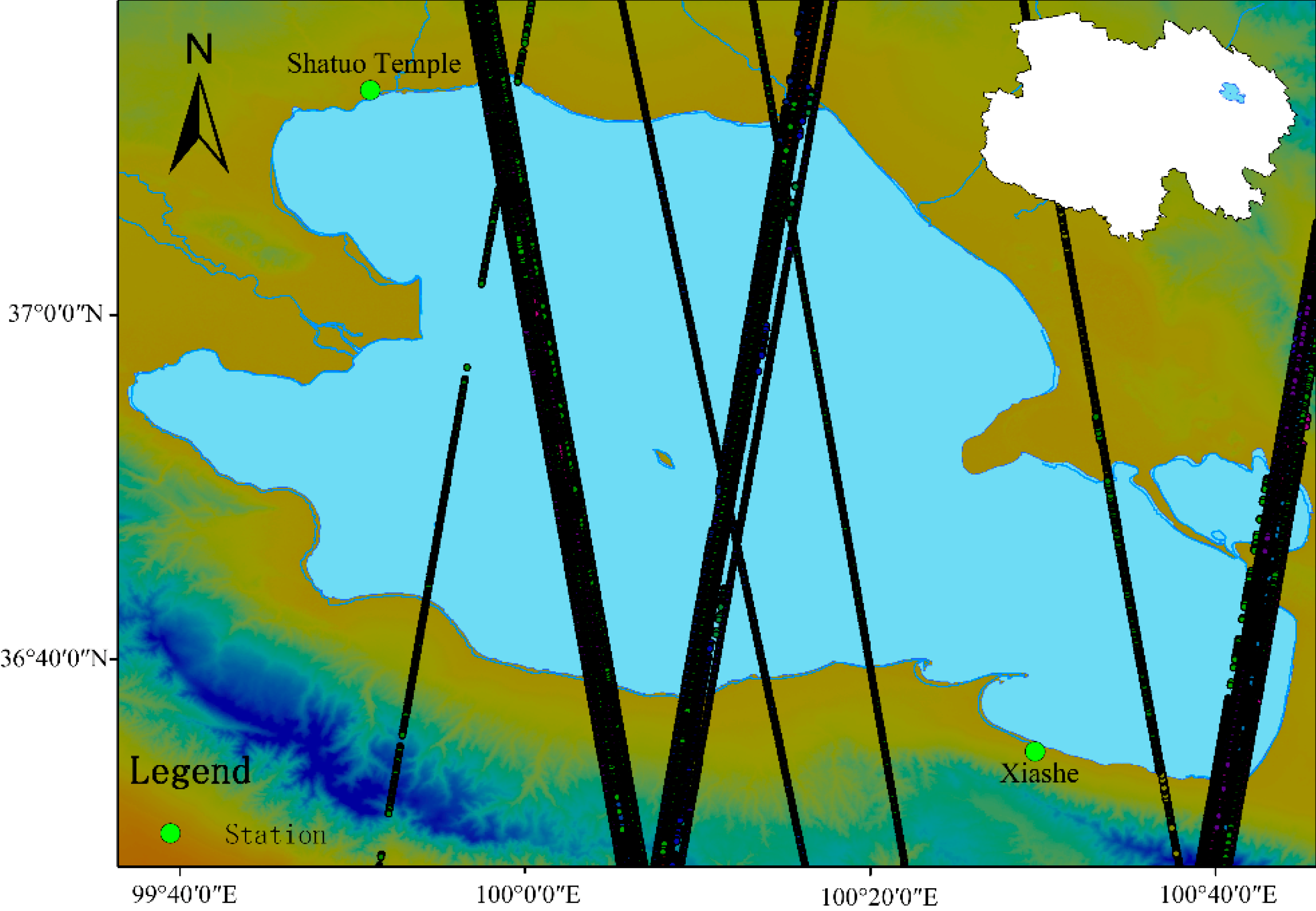
2. Lake Qinghai Settings

Lake Qinghai, also known as Tsongon Po, is an endorheic brackish lake (salinity 12.5 g/L) in the northeast margin of the Tibetan Plateau. As the biggest lake in China, it extends from 36°32′ to 37°15′N and 99°36′ to 100°47′E (Figure 1), with an altitude 3193 m a.s.l, an area of 4317.69 km², and a water volume 7.16 × 10¹⁰ m³ [11]. The mean depth of the lake is 21 m and the maximum 25.5 m [20]. The maximum length and width of the lake are approximately 106 and 67 km, respectively. The lake’s catchment area is about 29,660 km²; this yields an extension rate of 1 : 7 between the lake surface and its catchment area. The water is fed mainly by direct rainfall and runoff through more than 50 seasonal rivers or brooks. There are five large rivers and their tributaries that comprise the Lake Qinghai river system, namely Buha, Shaliu, Hargai, Quanji, and Heima. Among them, Buha River is the longest and largest river, which contributes almost half of the total runoff of the lake. Climatologically, the Lake Qinghai catchment belongs to the semi-arid zone with cold and dry winters and humid summers. The mean annual rainfall (1959–2000) is 357 ± 10 mm. Rainfall is concentrated in summer, and the rainfall from May to September accounts for 80% of the total annual rainfall [21]. Because of its high altitude, the annual mean temperature (1951–2007) is 1.2 °C, and the annual mean evaporation is 924 ± 10 mm, which is three times higher than precipitation [20]. As a result of its special geographical location and climatic characteristics, the ecological environment of the Lake Qinghai catchment is relatively fragile. Especially in the context of global change, the Lake Qinghai catchment has not only become one of the most sensitive regions to climate change in the entire Qinghai-Tibet Plateau, but it has also exhibited a series of environmental problems, such as desertification. It is therefore of great importance to quantitatively estimate and evaluate the water volume variations of Lake Qinghai. As shown in Figure 1, there are two in situ measurement stations around the Qinghai Lake, namely the Xiashe and Shatuo Temple. However, the period of available dates from the Shatuo Temple station are from 1958 to 1992, which do not coincide with the overpass time of ICESat. Therefore, only the observations from the Xiashe station were adopted for validation; the period of available data there is from 1984 to 2010.

Figure 1. Location of Lake Qinghai (blue polygon) in Qinghai Province (white polygon), gauging stations (green points) and all of the ICESat tracks (black lines).

Figure 1. Location of Lake Qinghai (blue polygon) in Qinghai Province (white polygon), gauging stations (green points) and all of the ICESat tracks (black lines).

3. Satellite Data Used and Methodology

3.1. Satellite Data

3.1.1. ICESat/GLAS

Ice, Cloud, and land Elevation Satellite (ICESat), as the first space-borne laser altimetry satellite orbiting the Earth, was launched in January 2003 and retired in February 2010 [22,23]. The Geoscience Laser Altimeter System (GLAS) is the sole payload of ICESat and it works at a frequency of 40 Hz with two channels, 532 nm and 1064 nm. The 1,064 nm channel is used to measure elevation in land, ice sheet, sea ice and ocean [24,25]. Laser footprints on the ground are about 72 m in diameter spaced at 172 m interval along the sub-satellite track [26]. To extend mission life, the operational mode included 33-day to 56-day campaigns, several times per year. Thus, during its lifetime, the GLAS sensor did not monitor elevations continuously, but only in designated campaigns. ICESat/GLAS level 2 altimetry product (GLA14) provides surface elevations for land, including rivers and lakes, plus laser footprint centroid geolocation, range measurements, geoid and many other parameters. Although the main mission of the GLAS instrument is to detect elevation changes in the polar ice caps, ICESat-GLA14 elevation data over water surface has been widely examined in various parts of the world and have shown accuracy of better than 10 cm [27,28,29,30,31,32,33,34,35]. All ICESat/GLAS14 release-33 data covering Lake Qinghai during 2003–2009 were downloaded from NASA’s National Snow and Ice Data Center (NSIDC) and processed. Time series elevation data, together with latitude, longitude and geoid information, are extracted to estimate the water level fluctuation of Lake Qinghai from 2003 to 2009.

3.1.2. Optical Satellite Images

Landsat TM/ETM+ images, because of their high spatial resolution, have been successfully used to extract water surface extent [36,37,38]. However, there are two problems that limit the Landsat TM/ETM+ application greatly in our study. Firstly, the number of TM/ETM+ images we can use at no cost is so inadequate that they are almost impossible to coincide with the dates of altimetry-derived water levels. Secondly, the Scan Line Corrector (SLC) compensating for the forward motion of the satellite in the ETM+ sensor failed on 31 May 2003, which is nearly the time ICESat began operating. There are wedge-shaped gaps and missing pixels in the ETM+ images acquired after the failure, which result in approximately 22% of missing image data for each scene [39]. Therefore, the MOD09Q1 product rather than Landsat TM/ETM+ was used in our study to extract the surface areas for Lake Qinghai on days when ICESat passed over our study area.

MODIS (Moderate Resolution Imaging Spectroradiometer) sensors were launched on board the National Aerodynamics and Space Administration (NASA) Earth Observing System (EOS) Terra and Aqua satellites on December 1999 and May 2002, respectively [40]. In this study, MOD09Q1 product with spatial resolution of 250 m was used to extract the surface areas for Lake Qinghai. MOD09Q1 provides surface reflectance of Band 1 (620–670 nm) and Band 2 (841–876 nm) in an 8-day gridded level-3 product. It should be noted that although in theory the satellite images should coincide exactly with the dates of altimetry-derived water levels, it is impossible to match them exactly in reality because of the inconsistency in temporal resolution between MOD09Q1 and ICESat-GLA14. Based on the daily in situ measurements from the Xiashe station, it is found that the average water level variation of Lake Qinghai is about 1.6 cm during an 8-day period. Therefore, it is assumed that the variations in surface area of Lake Qinghai during a short period (8 days) are minimal. MOD09Q1 8-day gridded images obtained on days close to most of the dates of ICESat overpass and were used to derive water surface areas at the corresponding water levels.

Due to their high accuracy in extracting water surface extent, Landsat TM/ETM+ images covering the study area from 1999 to 2009 were also adopted to monitor lake surface extent of Lake Qinghai, which was mainly used to extend the time series of water level records retrieved from ICESat-GLA14 product. All of the images used are cloud free or have a slight cloud cover (less than 5%). Gaps in the Landsat ETM+ SLC-off images were removed using a simple gap-filling extension toolbox (landsat_gapfill.sav) in the ENVI software [41]. This gap-filling method is based on the local linear histogram matching technique chose by USGS [42].

3.2. Methodology

3.2.1. ICESat Data Processing

It is already well recognized [30] that GLAS data have the potential for monitoring the level of inland water bodies. In this study, the method developed by Zhang et al. [11] was used to extract the footprints of Lake Qinghai. Based on Equation (1), the GLAS elevations are transformed from Topex/Poseidon ellipsoid to the WGS84 ellipsoid, so that a consistent comparison between GLAS elevations and the lake level records collected from hydrometric stations can be made in the same reference system:

ICESat_elevation = ICESat_elevation_Topex − EGM96_geoid − 0.7

(1)

where ICESat_elevation is the data referenced to the WGS84 ellipsoid, ICESat_elevation_Topex and EGM96_geoid are directly retrieved from ICESat/GLA14 data, and the 0.7 m is the offset from Topex ellipsoid to WGS84 ellipsoid [43]. Because of the impact of atmospheric conditions and heterogeneity in land surface, statistical analysis is usually indispensable to further remove some outliers caused by these factors. Standard deviation was adopted to define the threshold of outliers by Zhang et al [11]. However, their research shows that the allowable standard deviation is not a constant and varies with the season. For example, during the winter season, the allowable standard deviation could be up to 30 cm. The variability of the threshold may bring some subjectivity. Thus, a simple method was developed in our study to further remove some outliers. For each ICESat track that passed through Lake Qinghai, all of the footprints extracted by the water body mask (Section 3.2.2) were ranked by ICESat_elevation value, and the difference between two adjacent footprints was calculated successively. Then the footprints that cause a difference higher than 10 cm were labeled as outliers and removed. The average ICESat_elevation value of the remaining footprints was determined as the representative water level of the whole lake surface at the corresponding time. The definition of the 10 cm threshold was based on the general understanding that ICESat elevations on water surfaces would have an accuracy of 10 cm or better [11].

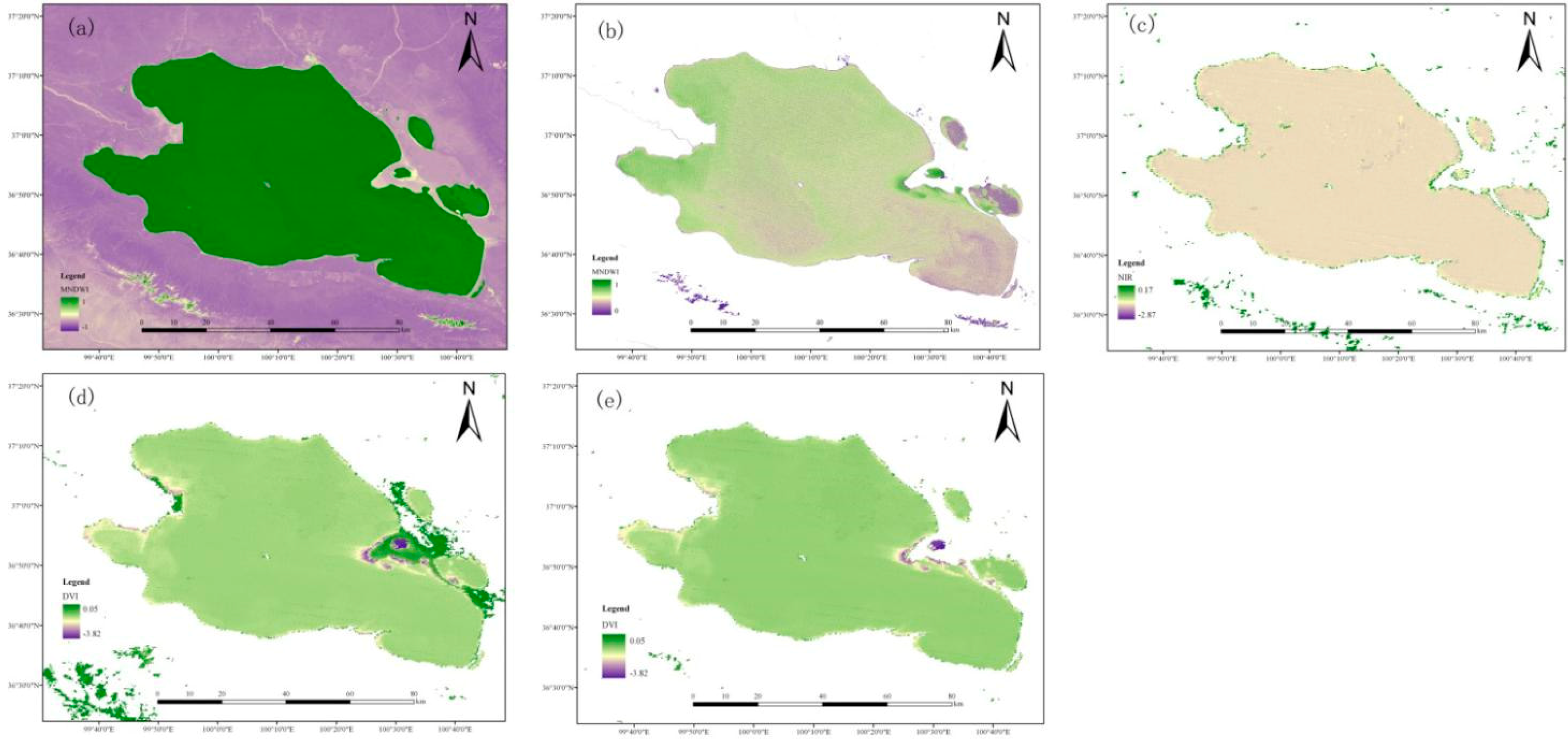
3.2.2. Surface Area Extraction

Specific RS methods were developed for water surface extraction, such as the Normalized Difference Water Index, NDWI [44,45,46,47]. The Modified Normalized Difference Water Index (MNDWI), developed by Xu [48], is a modification of NDWI, which gives improved differentiation between water bodies and other land features. The definition of MNDWI is given in Equation (2).

$$MNDWI = \frac{Green – MIR}{Green – MIR}$$

(2)

The difference between NDWI and MNDWI is that the latter uses the middle infrared band (MIR) instead of the near infrared band (NIR). Because of their high absorption in the MIR band and high reflectance in the Green band, water features usually have positive MNDWI values, while the MNDWI values of non-water features are usually negative. Therefore, a proper definition of specific thresholds of MNDWI reclassification can be used to separate water from other land cover components. In this paper, MNDWI was adopted to extract water surface extent from Landsat TM/ETM+ images. A three-step procedure was used. Step 1 was the calculation of MNDWI for all the Landsat images obtained above. In step 2, for each pixel the number of times when the MNDWI value was positive from 1999 to 2009 was counted, and the pixels with a frequency greater than 90% were assumed as water surface. Then a ten-pixel buffer zone was created over the continuous water surface, which was used as the water mask of Lake Qinghai. Both the extraction of lake surface and retrieval of water level were conducted in this mask. Step 3 was the delineation of lake surface extent for each Landsat image. Despite the considerable number of studies addressing water delineation, there have been divergent opinions concerning how thresholds should be defined [45,49,50]. In this paper, following the manual adjustment procedure by Xu [48] and recommendation by Ji et al. [32], different MNDWI threshold values were tested, and finally the threshold value was set as 0 for Lake Qinghai, which is consistent with the threshold that was used in the creation of water mask for Lake Qinghai.

There are only two bands in the MOD09Q1 product, namely the red band and the near infrared band. Therefore, it is impossible to calculate MNDWI or NDWI from MOD09Q1. However, due to the stronger absorptive capacity of water in the NIR range [51], the NIR band has been referenced as well-suited for detecting open aquatic surfaces. In addition, the Differential Vegetation Index (DVI), defined as the surface reflectance difference between the NIR band and the red band, was also proven useful in separating water from other land cover components [52,53]. Therefore, based on these two indicators, a two-threshold reclassification procedure was developed to delineate water extent of Lake Qinghai from MOD09Q1 product (Equation (3)).

$$\{\begin{array}{l}DVI < {threshold}_{\text{1}}\\ NIR < {threshold}_{\text{2}}\end{array}$$

(3)

Similar to MNDWI, the threshold definition for NIR and DVI is also specific to each study case. In this process, the surface area extracted above from Landsat TM/ETM+ images was adopted as criteria to calibrate the threshold for DVI and NIR. The values that fit best with the surface area extracted from Landsat TM/ETM+ images were adopted as the final threshold. After repeated tests of different threshold values and careful checks on the resulting water body boundary, the threshold values of NIR and DVI for Lake Qinghai were set as 0.17 and 0.05, respectively. Finally, the lake surface areas on days when ICESat overflew Lake Qinghai were obtained by summing up the areas of the pixels identified as aquatic surface. Figure 2 is an example of the surface area extracted from Landsat TM/ETM+ images and MOD09Q1 product.

Figure 2. Surface area extracted from Landsat TM/ETM+ images and MOD09Q1 product. (a) is the MNDWI calculated by using the Landsat TM/ETM+ images on 20 September 2006. (b) is the surface area of Lake Qinghai extracted from (a) using MNDWI > 0 as the threshold. (c) is the surface area of Lake Qinghai extracted from MOD09Q1 product on Julian day 257 in 2006 by using NIR < 0.17 as the threshold. (d) is the surface area of Lake Qinghai extracted from MOD09Q1 product on Julian day 257 in 2006 by using DVI < 0.05 as the threshold. (e) is the final surface area of Lake Qinghai extracted from MOD09Q1 product by using Equation (3).

Figure 2. Surface area extracted from Landsat TM/ETM+ images and MOD09Q1 product. (a) is the MNDWI calculated by using the Landsat TM/ETM+ images on 20 September 2006. (b) is the surface area of Lake Qinghai extracted from (a) using MNDWI > 0 as the threshold. (c) is the surface area of Lake Qinghai extracted from MOD09Q1 product on Julian day 257 in 2006 by using NIR < 0.17 as the threshold. (d) is the surface area of Lake Qinghai extracted from MOD09Q1 product on Julian day 257 in 2006 by using DVI < 0.05 as the threshold. (e) is the final surface area of Lake Qinghai extracted from MOD09Q1 product by using Equation (3).

3.2.3. Estimating Water Volume Variations

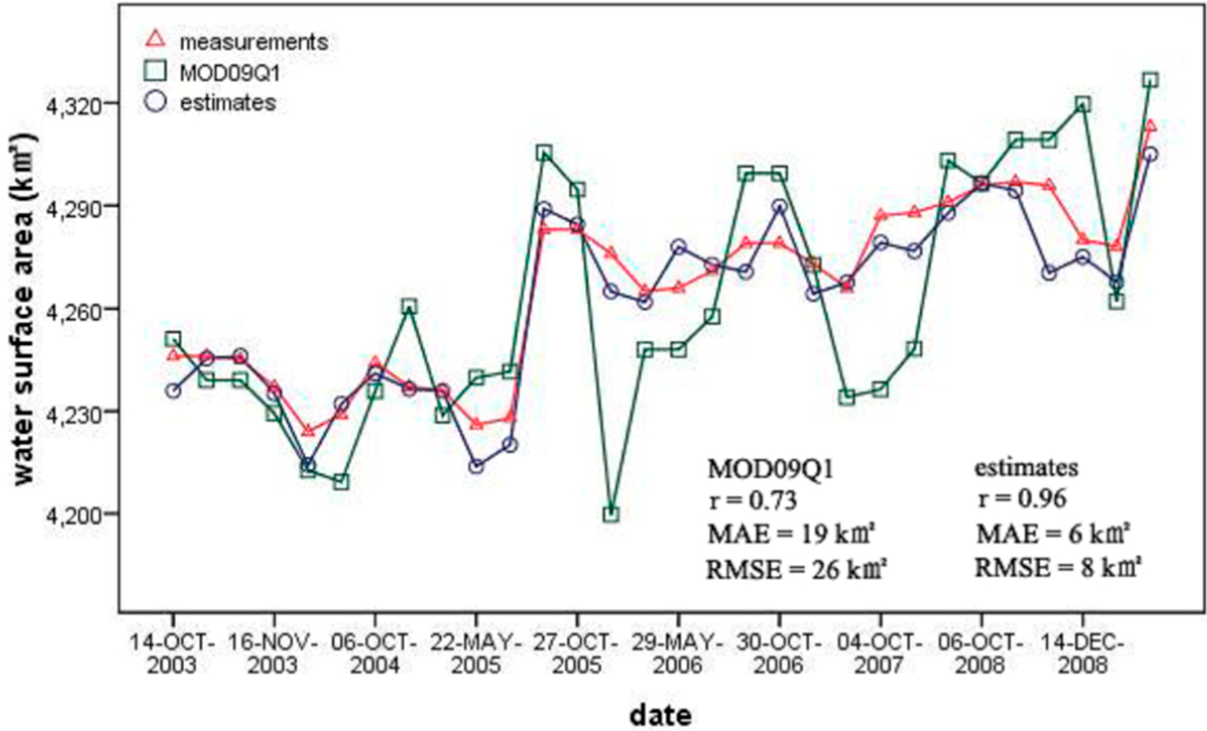
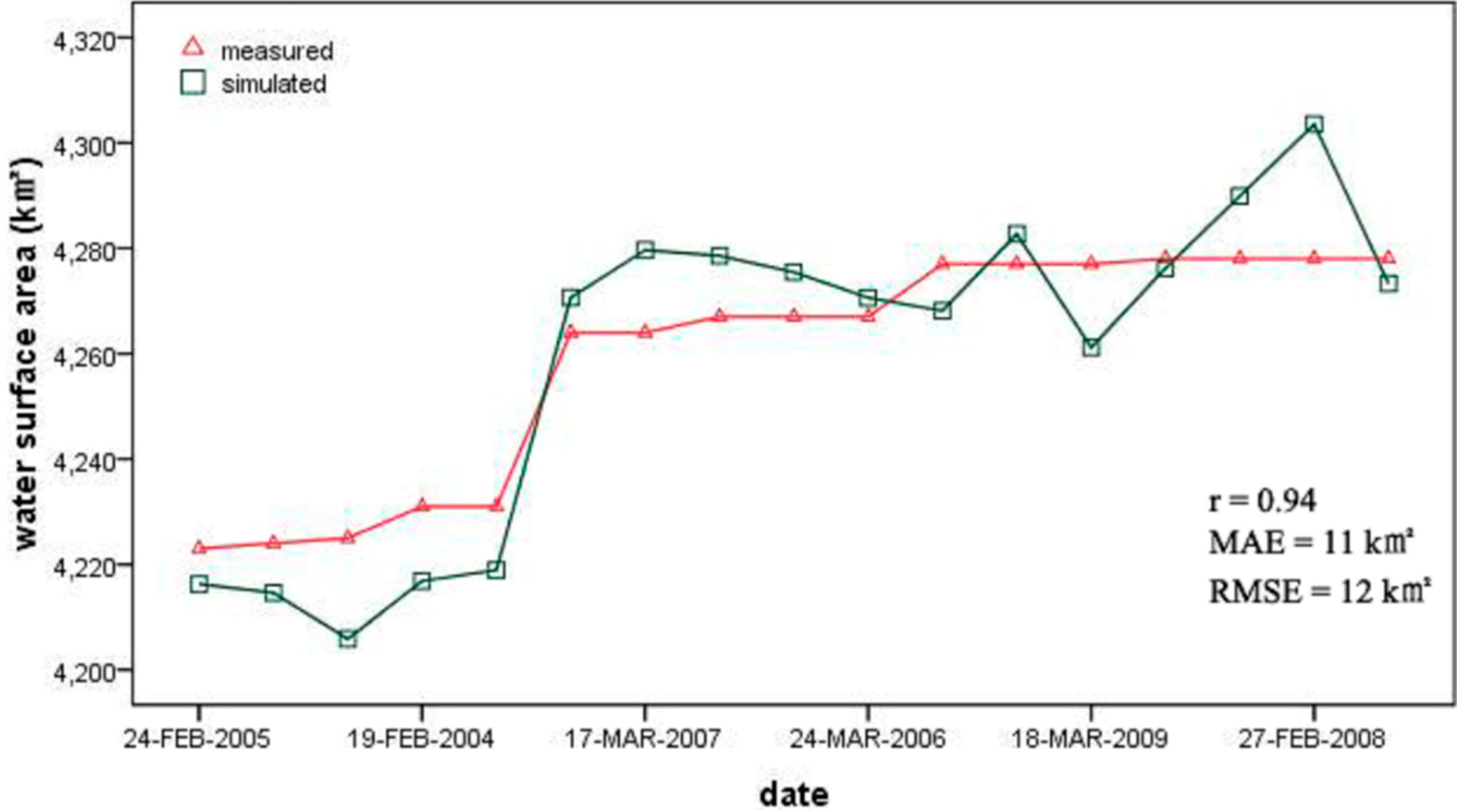
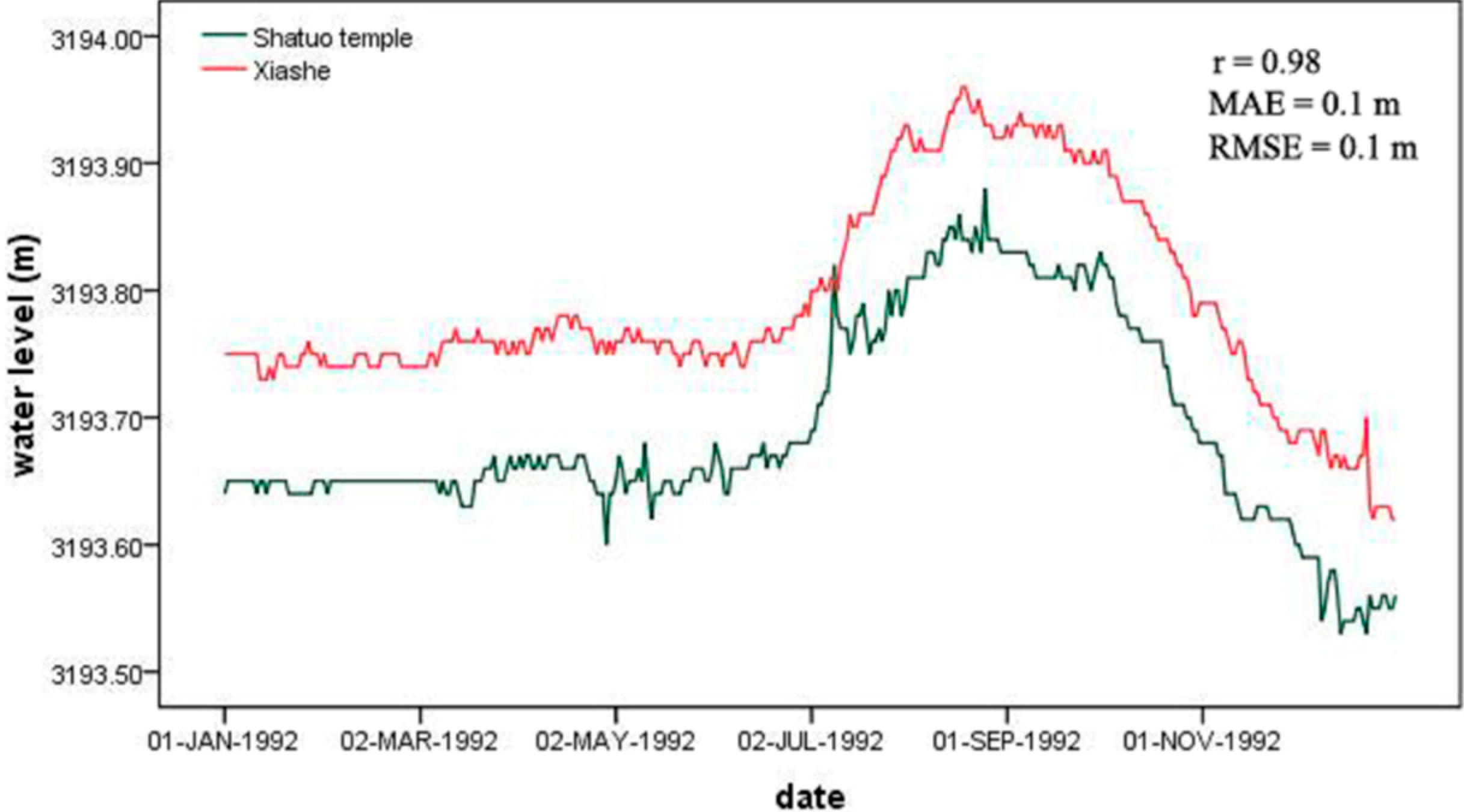
The determination of water volume variations needs both the changes in the water level and the variations in the lake surface extent. Although water surface extent corresponding to water level retrieved from ICESat can be extracted from MOD09Q1, the accuracy of the water area extracted is in doubt because of its low spatial resolution of 250 m. It is well known that, for a given lake, there is a certain relationship between its water level and surface extent. For the whole lake, exponential function is in most cases the best curve that fits this relationship. However, for a given section of this curve, especially when the water level is relatively high, the curve usually approximates closely the linear relationship. In this study, based on the water level data retrieved from ICESat and the corresponding water surface areas extracted from MOD09Q1, the statistical relationship between these two variables of Lake Qinghai was established using the linear regression method. Then the linear relationship established above was used in the following three aspects: (1) Improving the accuracy of water surface extent extracted from MOD09Q1: the water surface extent on days when ICESat passed over Lake Qinghai was estimated again using water level data derived from ICESat as inputs; (2) Extending the time series of water level retrieved from ICESat: the water level on days when Landsat passed over Lake Qinghai was estimated using water surface area extracted from TM/ETM+ images as inputs; (3) Estimating water volume variations: combining time series of water level data and the relationship established above makes it possible to estimate changes in lake storage directly using Equation (4).

$$\Delta \text{W = }{{\displaystyle \int }}_{h_{\text{1}}}^{h_{\text{2}}}f\text{(}h\text{)d}h$$

(4)

where $\Delta W$ is the variation in lake water volume during a given water level change (h₂ – h₁), f(h) is the estimated water surface extent corresponding to water level h. It should be noted that the relationship between water level and surface extent established in our study only works when the water level of Lake Qinghai is similar to the level data retrieved in our study. In cases when the water level is much higher or lower, the relationship established above would lose its effectiveness.

3.2.4. Validation

The validation of water levels derived from satellite is generally conducted by comparison with in situ measurements from gauging stations [5,11,54]. Daily water level measurements from the Xiashe station (Figure 1) were taken from Zhang et al. [11] to make comparisons with the water levels retrieved from ICESat. It is located in 36°35′16.0″N/100°29′28.4″E, the southeastern part of Lake Qinghai. It should be noted that in situ water levels from the Xiashe station have their own reference datum (the Yellow Sea Datum), which is different from the geoids adopted by ICESat. By combination of the datum mark and gauge measurements, the difference between the renewed Yellow Sea Datum and the WGS84 datum is about 40 cm in the Lake Qinghai area [55]. Therefore, the in situ measurements are transformed into the WGS84 datum for comparison with ICESat altimetry data.

For water surface area and water volume, a systematic survey on Lake Qinghai was conducted by the Hydrology and Water Resources Survey Bureau of Qinghai province in 2011. During this campaign, the underwater topography was measured by using sonar sensors on ship transects, and bathymetry maps with high resolution were obtained. Then the curve between water level and water surface area (L-A), and the curve between water level and water storages (L-V) were lineated based on this survey. Thus, the aquatic surface and water storages corresponding to any water level can be known through these curves, which were used to validate the water surface area and water volume variation in our study. However, because of its confidentiality, the water surface area and water volume provided by the Hydrology and Water Resources Survey Bureau of Qinghai Province was just used as validation and was not presented in detail.

For validation purpose, three statistics named with the correlation coefficient (r), the mean absolute error (MAE) and the root mean square error (RMSE) were calculated, which are expressed as

(5)

$$MAE = \frac{\text{1}}{n}{\displaystyle \sum }_{i\text{ = 1}}^n\left|y_i{\text{ – }y}_i^{\prime }\right|$$

(6)

$$RMSE = \sqrt{\frac{\text{1}}{n} {\displaystyle \sum }_{i\text{ = 1}}^n{{\text{(}y}_i\text{ –} y_i^{\prime }\text{ )}}^2}$$

(7)

where, y is the variable such as water level, surface area and water volume measured at the station, y’ is the corresponding variable estimated in our study, $\overline{y}$ and $\overline{y^{\prime }}$ are the mean value of y and y’, respectively, i is the index of the variable, and n is the number of the sample size.

4. Results

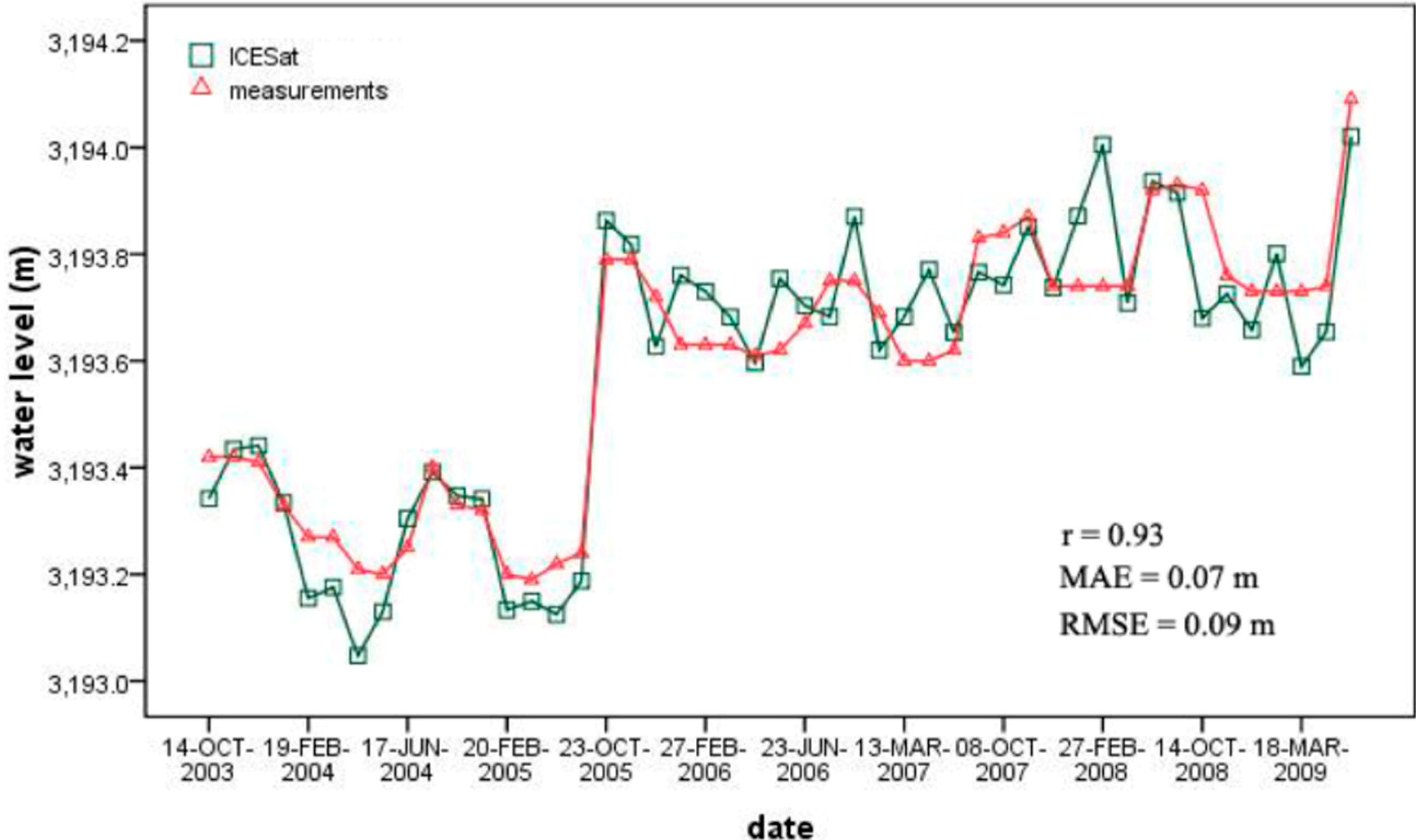
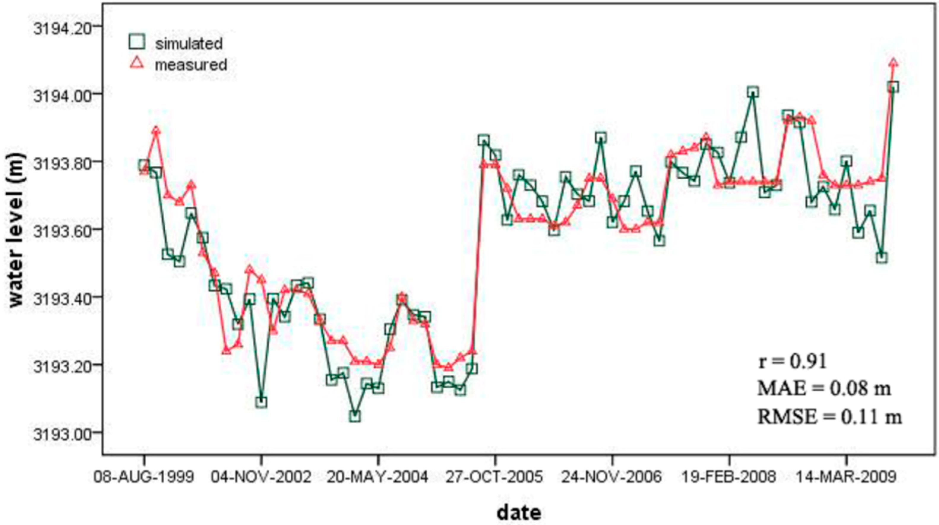
4.1. ICESat/GLA14-Derived Water Levels

In total, there are 47 tracks covering Lake Qinghai from 2003 to 2009. All of these tracks were shown in Figure 1. Figure 3 is the time series curve from 2003 to 2009, which indicates the difference between daily water level retrieved from ICESat and in situ measurements from the Xiashe station. In general, the estimated results effectively captured the trend of annual variation of water level. Both of them indicated an increase tendency for Lake Qinghai. Judging from the magnitude, the results retrieved from ICESat showed that water level had increased from 3193.34 m on 14 October 2003 to 3194.02 m on 2 October 2009. The difference of lake level for the six-year period is about 0.68 m, and the annual average rate of increase is about 0.11 m/yr, which is very close to the results obtained from in situ measurements (from 3193.42 m on 14 October 2003 to 3194.09 m on 2 October 2009). A good agreement was found between the estimated and measured water levels with correlation coefficient r as high as 0.93. The mean absolute error (MAE) and root-mean-square-error (RMSE) between these two elevations are 0.07 m and 0.09 m, respectively, which are similar to the results conducted by Zhang et al. [11] over the same study area (Table 1). Both of these studies support that ICESat elevation has shown accuracy of better than 10 cm in retrieving water levels. The study conducted by Song et al. [7] showed that the time series elevation data retrieved from ICESat could also reveal clear seasonal variations in water level over lakes on the Tibetan Plateau. Unfortunately, this method has lost its effectiveness in monitoring the seasonal variations of Lake Qinghai for the following two reasons. Firstly, on average there are only seven tracks covering Lake Qinghai per year, and they are mainly concentrated in a few months (for example, mainly in February and October in the year 2008), which makes it impossible to monitor water level variations in other months. Secondly, the MAE on some individual days is higher than 10 cm, which introduces large uncertainty in estimation seasonal variation due to the small fluctuation of water level (about 20 cm) during the year. Therefore, we don’t think ICESat alone can be used to monitor the seasonal variations of water level in Lake Qinghai.

Figure 3. Time series of water levels retrieved from ICESat versus measurements. The green square represents the water level estimated by ICESat, and the red triangle represents the water level observed at the Xiashe station.

Figure 3. Time series of water levels retrieved from ICESat versus measurements. The green square represents the water level estimated by ICESat, and the red triangle represents the water level observed at the Xiashe station.

Table 1. Water level of Lake Qinghai derived from ICESat elevation data and the in situ measurements of water level at Xiashe station. The water level unit is in meters

Date	ICEsat Elevation	In situ Measurement	Date	ICEsat Elevation	In situ Measurement
10/14/2003	3193.34	3193.42	06/23/2006	3193.70	3193.67
10/18/2003	3193.43	3193.42	10/27/2006	3193.68	3193.75
10/22/2003	3193.44	3193.41	10/30/2006	3193.87	3193.75
11/16/2003	3193.33	3193.33	11/24/2006	3193.62	3193.69
02/19/2004	3193.16	3193.27	03/13/2007	3193.68	3193.60
02/22/2004	3193.18	3193.27	03/17/2007	3193.77	3193.60
03/18/2004	3193.05	3193.21	04/11/2007	3193.65	3193.62
05/20/2004	3193.13	3193.20	10/04/2007	3193.77	3193.83
06/17/2004	3193.31	3193.25	10/08/2007	3193.74	3193.84
10/06/2004	3193.39	3193.40	11/02/2007	3193.85	3193.87
11/03/2004	3193.35	3193.33	02/19/2008	3193.74	3193.74
11/08/2004	3193.34	3193.32	02/22/2008	3193.87	3193.74
02/20/2005	3193.13	3193.20	02/27/2008	3194.01	3193.74
02/24/2005	3193.15	3193.19	03/18/2008	3193.71	3193.74
05/22/2005	3193.13	3193.22	10/06/2008	3193.94	3193.92
05/26/2005	3193.19	3193.24	10/09/2008	3193.92	3193.93
10/23/2005	3193.86	3193.79	10/14/2008	3193.68	3193.92
10/27/2005	3193.82	3193.79	12/14/2008	3193.73	3193.76
11/21/2005	3193.63	3193.72	03/10/2009	3193.66	3193.73
02/24/2006	3193.76	3193.63	03/14/2009	3193.80	3193.73
02/27/2006	3193.73	3193.63	03/18/2009	3193.59	3193.73
03/24/2006	3193.68	3193.63	04/08/2009	3193.66	3193.74
05/26/2006	3193.60	3193.61	10/02/2009	3194.02	3194.09
05/29/2006	3193.75	3193.62

Table 1. Water level of Lake Qinghai derived from ICESat elevation data and the in situ measurements of water level at Xiashe station. The water level unit is in meters

Date	ICEsat Elevation	In situ Measurement	Date	ICEsat Elevation	In situ Measurement
10/14/2003	3193.34	3193.42	06/23/2006	3193.70	3193.67
10/18/2003	3193.43	3193.42	10/27/2006	3193.68	3193.75
10/22/2003	3193.44	3193.41	10/30/2006	3193.87	3193.75
11/16/2003	3193.33	3193.33	11/24/2006	3193.62	3193.69
02/19/2004	3193.16	3193.27	03/13/2007	3193.68	3193.60
02/22/2004	3193.18	3193.27	03/17/2007	3193.77	3193.60
03/18/2004	3193.05	3193.21	04/11/2007	3193.65	3193.62
05/20/2004	3193.13	3193.20	10/04/2007	3193.77	3193.83
06/17/2004	3193.31	3193.25	10/08/2007	3193.74	3193.84
10/06/2004	3193.39	3193.40	11/02/2007	3193.85	3193.87
11/03/2004	3193.35	3193.33	02/19/2008	3193.74	3193.74
11/08/2004	3193.34	3193.32	02/22/2008	3193.87	3193.74
02/20/2005	3193.13	3193.20	02/27/2008	3194.01	3193.74
02/24/2005	3193.15	3193.19	03/18/2008	3193.71	3193.74
05/22/2005	3193.13	3193.22	10/06/2008	3193.94	3193.92
05/26/2005	3193.19	3193.24	10/09/2008	3193.92	3193.93
10/23/2005	3193.86	3193.79	10/14/2008	3193.68	3193.92
10/27/2005	3193.82	3193.79	12/14/2008	3193.73	3193.76
11/21/2005	3193.63	3193.72	03/10/2009	3193.66	3193.73
02/24/2006	3193.76	3193.63	03/14/2009	3193.80	3193.73
02/27/2006	3193.73	3193.63	03/18/2009	3193.59	3193.73
03/24/2006	3193.68	3193.63	04/08/2009	3193.66	3193.74
05/26/2006	3193.60	3193.61	10/02/2009	3194.02	3194.09
05/29/2006	3193.75	3193.62

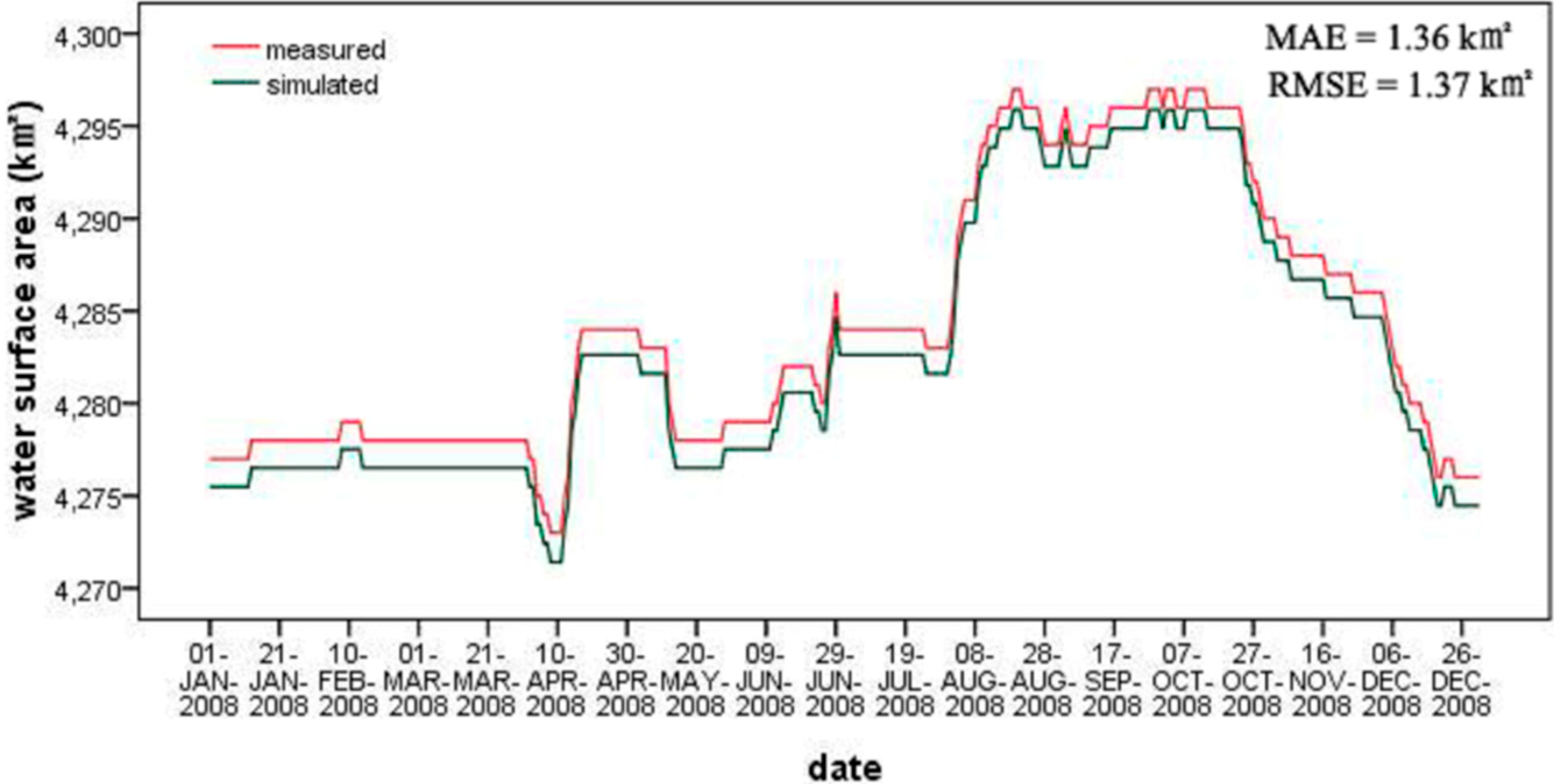
4.2. Surface Area Changes

The time series curve of all the surface area extracted from Landsat images was given in Figure 4. Compared with the surface area measured in Xiashe Station, good agreement was obtained with r as high as 0.81. The MAE and RMSE are 11 km² and 15 km², respectively, which only account for 0.3% of the surface area of Lake Qinghai. Therefore, it is feasible to extract surface area of inland water bodies with high accuracy from Landsat images.

Figure 4. Time series of surface areas extracted from Landsat TM images versus measurements and the extended water levels estimated by the L-A equation established in Section 4.3 and the surface areas extracted from Landsat TM images as inputs. The blue square represents the surface areas estimated from Landsat TM images, and the red triangle represents the surface areas observed at Xiashe station, which was retrieved from the water level observations and the L-A curve provided by the Hydrology and Water Resources Survey Bureau of Qinghai Province. The purple square represents the extended water levels that were estimated by using the L-A equation in Section 4.3 and the surface areas extracted from Landsat TM images as inputs, while the green triangle represents the water levels measured at the Xiashe station.

Figure 4. Time series of surface areas extracted from Landsat TM images versus measurements and the extended water levels estimated by the L-A equation established in Section 4.3 and the surface areas extracted from Landsat TM images as inputs. The blue square represents the surface areas estimated from Landsat TM images, and the red triangle represents the surface areas observed at Xiashe station, which was retrieved from the water level observations and the L-A curve provided by the Hydrology and Water Resources Survey Bureau of Qinghai Province. The purple square represents the extended water levels that were estimated by using the L-A equation in Section 4.3 and the surface areas extracted from Landsat TM images as inputs, while the green triangle represents the water levels measured at the Xiashe station.

The classification method in Equation (3) is not suitable for delineating surface extent when the water is mixed with ice. After eliminating the images with dense cloud and ice cover, water surface area for 30 days was extracted from MOD09Q1. The time series curve of estimated surface area versus measured surface area was shown in Figure 5. Although the MAE on some individual days is relatively large, the results could also capture the increase trend of Lake Qinghai from 2003 to 2009. The surface area has increased from 4285 km² on 14 October 2003 to 4362 km² on 2 October 2009. The difference of surface area for the six-year period is around 77 km², and the annual average rate of increase is about 13 km²/yr, which is close to the results obtained from in situ measurements (from 4286 km² on 14 October 2003 to 4355 km² on 2 October 2009). Compared with the surface area extracted from Landsat images, the accuracy of the surface extent extracted from MOD09Q1 is not very good, the MAE and RMSE is 19 km² and 26 km², respectively. Further research is required to improve the accuracy of the surface area extracted from MOD09Q1.

Figure 5. Time series of surface areas extracted from MOD09Q1 and surface areas estimated by using the L-A equation established in Figure 6 and the water levels retrieved from ICESat as inputs versus measurements. The purple circular represents the surface areas simulated by using the L-A equation in Figure 6 and the water levels retrieved from ICESat as inputs, the green square represents surface area extracted from MOD09Q1, while the red triangle represents the measured surface area.

Figure 5. Time series of surface areas extracted from MOD09Q1 and surface areas estimated by using the L-A equation established in Figure 6 and the water levels retrieved from ICESat as inputs versus measurements. The purple circular represents the surface areas simulated by using the L-A equation in Figure 6 and the water levels retrieved from ICESat as inputs, the green square represents surface area extracted from MOD09Q1, while the red triangle represents the measured surface area.

Figure 6. The empirical relationship between water levels and surface areas of Lake Qinghai, which was established by using the surface areas retrieved from MOD09Q1 and water levels retrieved from ICEsat as inputs.

Figure 6. The empirical relationship between water levels and surface areas of Lake Qinghai, which was established by using the surface areas retrieved from MOD09Q1 and water levels retrieved from ICEsat as inputs.

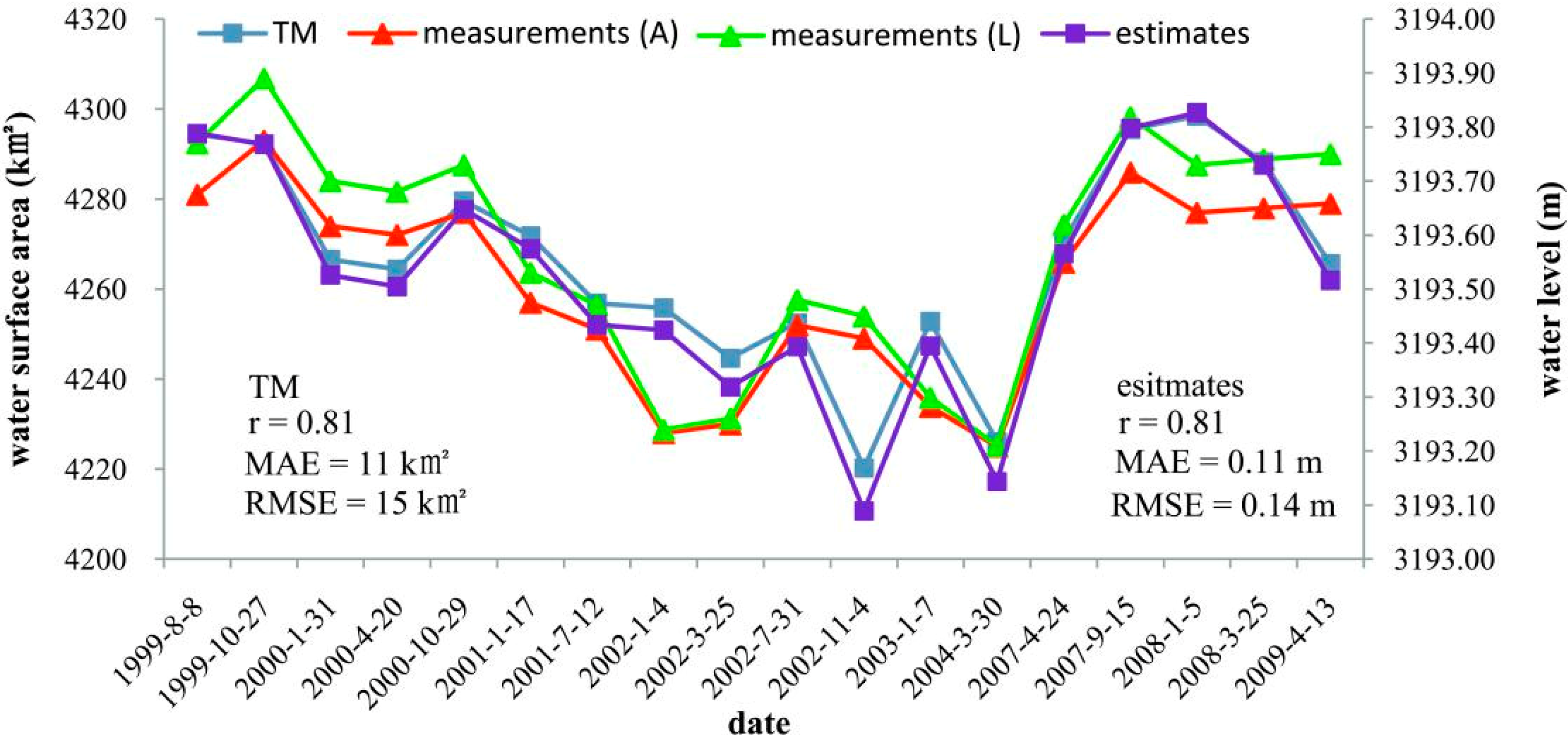
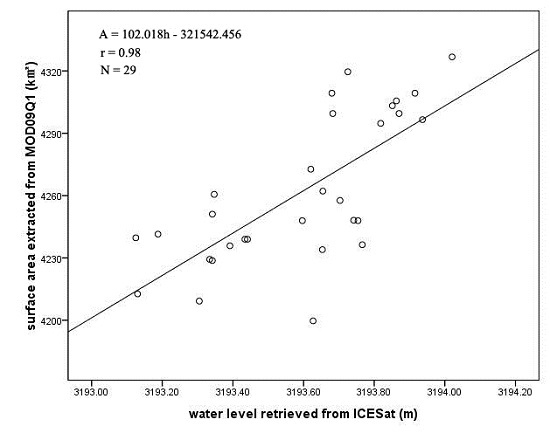
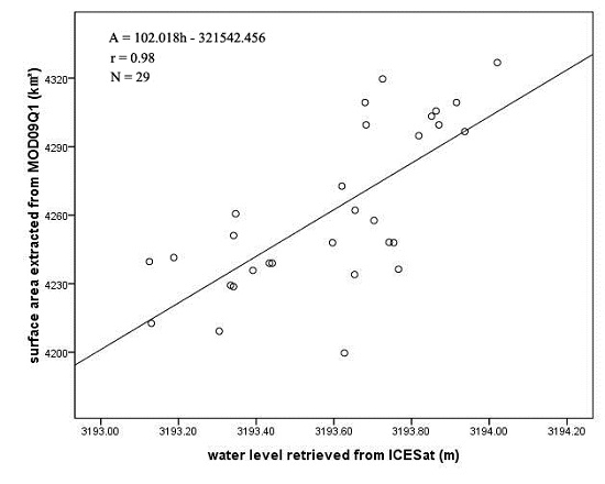
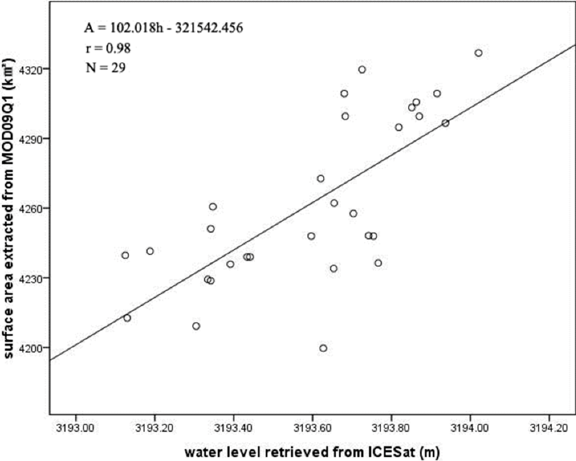
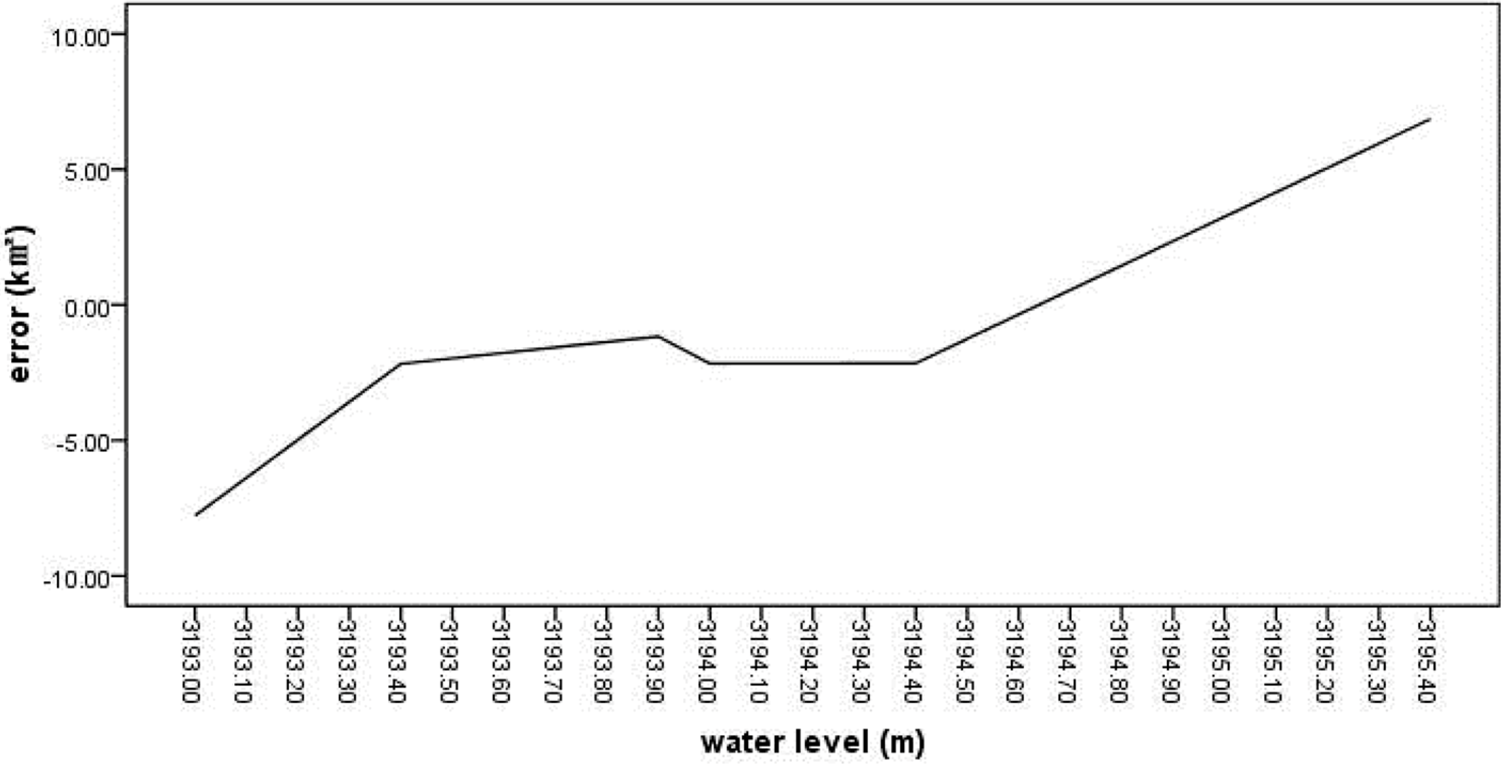
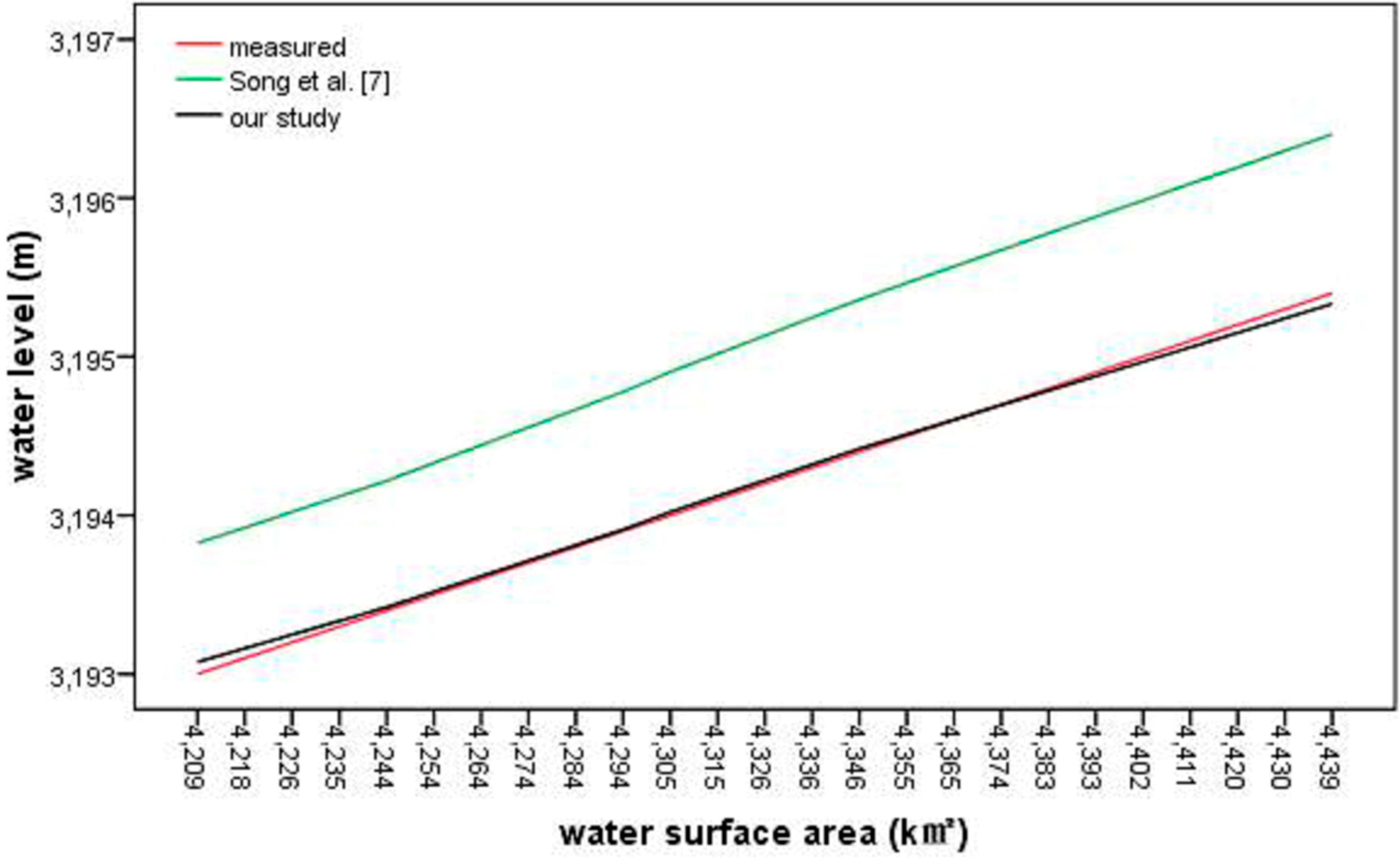
4.3. Relationship between Water Level and Surface Area

Based on the water level retrieved from ICESat and the corresponding surface extent extracted from MOD09Q1, the statistical relationship between water level (h) and surface area (A) of Lake Qinghai was established using linear regression method. The results were shown in Figure 6. Then the surface area corresponding to the water level retrieved from ICESat was estimated again using this linear equation. The time series curve of the estimated surface area and measured area was presented in Figure 5. It is obvious that compared with the surface area extracted from MOD09Q1, the accuracy of the surface area estimated using this linear relationship has been improved significantly. The results were in good agreement with the measured surface area with MAE = 6 km², and RMSE = 8 km², which are even lower than the MAE and RMSE of surface area extracted from Landsat images. Finally, the surface area corresponding to other ICESat-derived water levels that were not used in the establishment of linear equation was also estimated. The results were given in Figure 7. Similar accuracy was obtained with MAE = 11 km², and RMSE = 12 km², which are still better than the results extracted from MOD09Q1. Therefore, the linear relationship established above was applied to all of the water levels retrieved from ICESat.

Figure 7. Comparison of the estimated surface areas with measurements. The green square represents the surface areas estimated by using the L-A equation in Figure 6 and the water levels retrieved from ICESat as inputs. The difference between Figure 5 and Figure 7 is that the water level used in Figure 5 was adopted in the establishment of the L-A equation in Figure 6, while the water level used in Figure 7 was not.

Figure 7. Comparison of the estimated surface areas with measurements. The green square represents the surface areas estimated by using the L-A equation in Figure 6 and the water levels retrieved from ICESat as inputs. The difference between Figure 5 and Figure 7 is that the water level used in Figure 5 was adopted in the establishment of the L-A equation in Figure 6, while the water level used in Figure 7 was not.

In return, the water levels corresponding to the surface areas extracted from Landsat images were also estimated using the inverse function of the linear equation in Figure 6. The results were presented in Figure 4 with MAE = 11 cm and RMSE = 14 cm. Both of them are 4 cm higher than the MAE and RMSE of water levels retrieved from ICESat. Therefore, in our study, ICESat elevation data provides a better indicator for water fluctuation of Lake Qinghai than Landsat images. Combined with the estimated water levels from this linear equation, the time series of water levels retrieved from ICESat were extended to the year 1999. Figure 8 presents the results of the reconstructed water levels from 1999 to 2009. Overall, good agreement was achieved with r = 0.91, MAE = 8 cm, and RMSE = 11 cm.

Figure 8. The reconstructed water levels from 1999 to 2009. The green square represents the reconstructed water level, which in fact was the combination of the water level retrieved from ICESat and the water level extended in Figure 4.

Figure 8. The reconstructed water levels from 1999 to 2009. The green square represents the reconstructed water level, which in fact was the combination of the water level retrieved from ICESat and the water level extended in Figure 4.

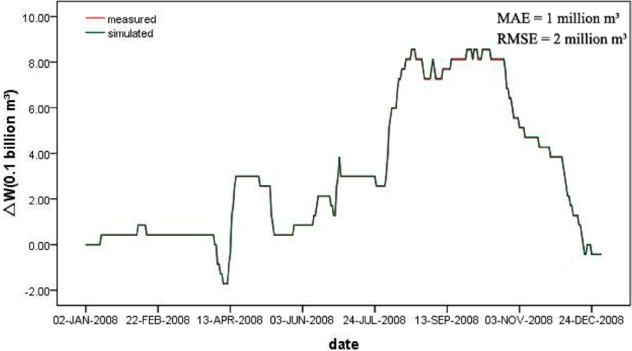
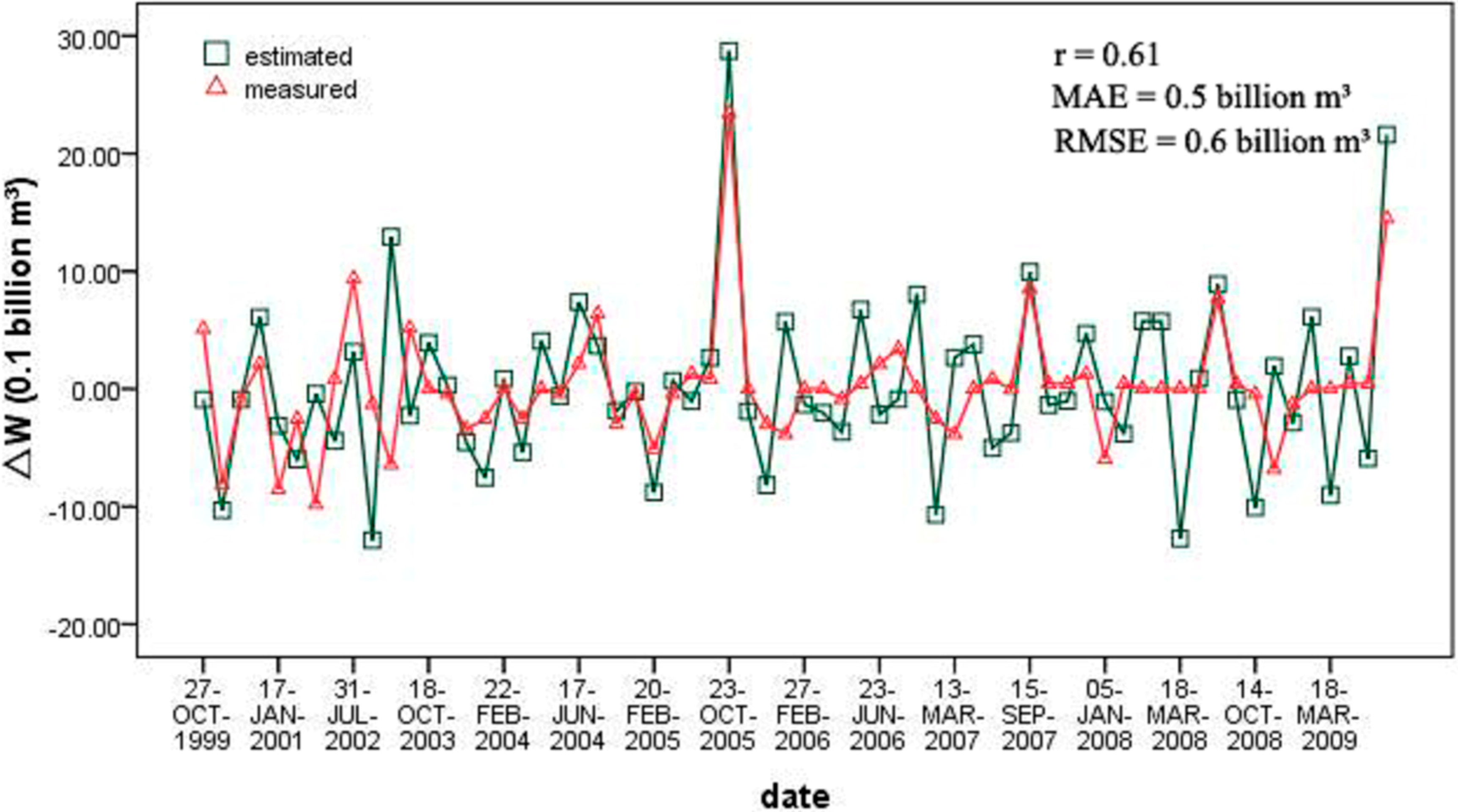
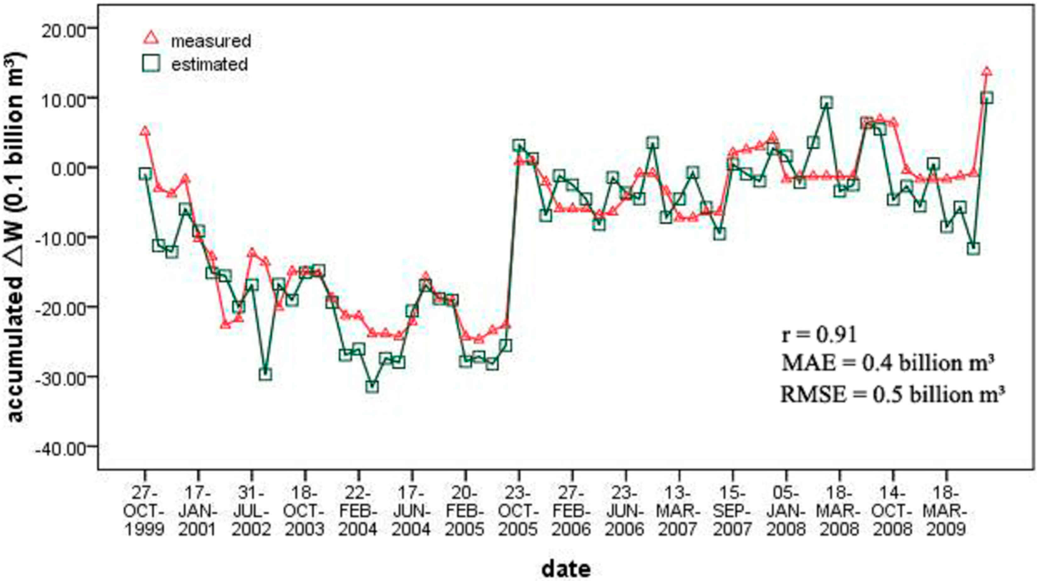
4.4. Water Volume Variations

Finally, based on the statistical relationship between water level and surface area established above, the water volume variations ($\Delta W$) of Lake Qinghai were estimated using the reconstructed water levels as inputs and the linear equation established in Figure 6 as f(h). Equation (5) is the equation retrieved from Equation (4) to estimate the variations of water storage, where h₁ and h₂ are adjacent water levels.

$$\Delta W\text{ = 0}{\text{.051009 }h}^{\text{2}}\text{ – 321.542456 }{h|}_{h_{\text{1}}}^{h_{\text{2}}}$$

(8)

For validation purposes, the unit in Equation (5) has been transformed into m³. All 65 original water levels (47 water levels retrieved from ICESat, and 18 water levels estimated from Landsat images) were used for the estimation of water volume variations. The results were shown in Figure 9. With the exception of individual days, the results effectively captured the trend of annual variation of water volume. Good agreement was obtained between the estimated and measured water volume variations with r as high as 0.61, MAE = 0.5 billion m³, and RMSE = 0.6 billion m³, which account for 0.7% of the total water volume of Lake Qinghai. By comparing $\Delta W$ in May with $\Delta W$ in October, the results also provided insight into the seasonal variation of Lake Qinghai. The water volume of Lake Qinghai increases between May and October (with positive $\Delta W$) and then gradually deceases until April of the following year (with negative $\Delta W$).

Figure 9. Comparison of the estimated water volume variations with measurements. The green square represents the water volume variations estimated by using Equation (5) and the reconstructed water level in Figure 8 as inputs. The red triangle represents the water volume variations observed at the Xiashe station, which was retrieved from the water level observations and the L-V curve provided by the Hydrology and Water Resources Survey Bureau of Qinghai Province.

Figure 9. Comparison of the estimated water volume variations with measurements. The green square represents the water volume variations estimated by using Equation (5) and the reconstructed water level in Figure 8 as inputs. The red triangle represents the water volume variations observed at the Xiashe station, which was retrieved from the water level observations and the L-V curve provided by the Hydrology and Water Resources Survey Bureau of Qinghai Province.

In order to further investigate the annual variation of water volume in Lake Qinghai, the $\Delta W$ in Figure 9 was accumulated. For validation purposes, the corresponding in situ measurement of $\Delta W$ was also accumulated, and the water volume on 8th August 1999 was adopted as the baseline. The results were shown in Figure 10. The estimated results were in good agreement with the in situ measurements in both the amplitude and phase with a high r of 0.91. The MAE and RMSE are 0.4 billion m³ and 0.5 billion m³, respectively. During the period from 1999 to 2009, the water volume variation of Lake Qinghai can be divided into three phases. From 1999 to 2004, the water volume had decreased by 1.9 billion m³; the annual average rate was 0.6 billion m³ per year. It then began to increase rapidly. During the period from 20 February 2005 to 21 November 2005, the water volume increased by 2.1 billion m³ in just nine months, but the water volume was still lower than that in 1999. In the four subsequent years, although intense seasonal variation occurred in 2009 (the water volume increased by 1.6 billion m³ in just seven months), the water volume variations exhibit a trend of increasing gradually. The annual average rate of increase is about 0.42 billion m³ per year, which is very close to the rate calculated from in situ measurements (0.39 billion m³ per year).

Figure 10. Time series of the estimated accumulated water volume variations versus measurements. The green square represents the accumulated water volume variations estimated by our work.

Figure 10. Time series of the estimated accumulated water volume variations versus measurements. The green square represents the accumulated water volume variations estimated by our work.

5. Discussion

5.1. The Accuracy of In Situ Measurements

In this study, the in situ daily water levels at Xiashe Station and the corresponding surface areas and water volumes during the period 1999–2009 were used for validation. The uncertainty of both altimetry measurements and in situ measurements can contribute to the error of final validation. Previous studies show that the actual lake level fluctuation occurs not only due to changes of water volume but it can also be locally influenced by air pressure changes, circulation processes, wind events and tides [5,9,56]. In order to investigate the representative of the water level measured at the Xiashe station, the in situ measurements from another gauging station, Shatuo Temple (Figure 1), were obtained. Unfortunately, the Shatuo Temple station was only operational during the period 1956–1992; the daily water level records during the year 1992 were thus adopted to make a comparison with the corresponding water levels measured at the Xiashe station. The results were presented in Figure 11. Although good agreement was found with a high r of 0.98, there was a significant systematic error existing between these two water level records. The error may be caused by a geoid since Lake Qinghai is so large. Overall, the water level records at the Xiasha station were 10 cm higher than that at the Shatuo Temple station. The MAE and RMSE were both equal to 10 cm, which was even a little higher than the MAE and RMSE calculated from the water levels retrieved from ICESat.

Figure 11. Comparison of the water levels measured at different gauging stations.

Figure 11. Comparison of the water levels measured at different gauging stations.

It should also be noted that the water levels derived from ICESat are average values along the ground tracks overflying Lake Qinghai, and the tacks are usually some distance away from the Xiashe station. This also brings in some uncertainties in the validation results. Given that the MAE in Figure 11 is almost the same as the MAE in Figure 3, there are good reasons to conclude that the average value along the ICESat tracks is a more representative indicator of the water level of the whole lake.

As for the surface extent and water volume, the in situ daily surface areas and water volumes were extracted from the L-A curve and L-V curve delineated by the Hydrology and Water Resources Survey Bureau of Qinghai Province. The accuracy of these two curves was unknown. Even if assuming the curves were absolutely accurate, the 10 cm error in the water level measurements would introduce 10 km² error in the surface area measurements and 0.4 billion m³ error in the water volume measurements. These errors should be kept in mind for the final validation

5.2. The Extension of Our Study

Using multi-source remote sensing data, the statistical relationship between water level and surface area of Lake Qinghai was estimated without any in situ measurements, which was then used for the reconstruction of water level time series and the estimation of water volume variations. In fact, compared with surface area and water volume, water level is relatively easy to measure, and is usually the only variable that is measured routinely for some lakes like Lake Qinghai. In these cases, the L-A and L-V curves can be estimated using the method developed in our study, and then daily surface area and water volume can be estimated from these curves using the corresponding daily water level measurements as inputs. Here the case of Lake Qinghai in the year 2008 was used as an example. Figure 12 presents the time series curve of the estimated and measured water area in the year 2008. Although there is a little underestimation of the water area with a negative systematic error, good agreement was achieved between the estimated and measured water area. The MAE and RMSE are only 1.36 km² and 1.37 km², respectively. The seasonal variations of water volume in 2008 are shown in Figure 13. Here, the water volume on 1 August 2008 was used as the baseline. It is obvious that the estimated L-V curve provides a perfect capture of the seasonal variation of water volume. The MAE and RMSE are only 1 million m³ and 2 million m³, respectively, which account for 2% and 4% of the daily volume variations. Therefore, the L-V curves established in our study are reliable. As mentioned in Section 4.3, the L-A curve established using the linear regression method in our study only works for a limited range of water levels. In order to investigate this range, different water level thresholds were used to compare the estimated surface area with the measured surface area. The curve of the bias (estimated area and measured area) was presented in Figure 14. With the water level increasing from 3193 m to 3195 m, the absolute error decreases first and then increases. When the water level is below 3194.6 m, the L-A curve tends to underestimate the surface area. When the water level is above 3194.7 m, the L-V curve tends to overestimate the surface area. The best application range of the L-A curve established in this study is about from 3193.4 m to 3194.4 m. In this range, the error is relatively stable, and is lower than 2 km². Beyond this range, the error tends to increase rapidly.

Figure 12. Time series of the estimated water surface areas versus measurements in the year 2008. The green line represents the surface areas estimated by using the L-A curve established in Figure 6 and the water level observations at Xiashe station as inputs.

Figure 12. Time series of the estimated water surface areas versus measurements in the year 2008. The green line represents the surface areas estimated by using the L-A curve established in Figure 6 and the water level observations at Xiashe station as inputs.

Figure 13. Seasonal variations of water volume in 2008. The green line represents the water volume variations estimated by using Equation (5) and the water level observations at the Xiashe station as inputs. The difference between the measured and simulated water volume variations is so small that these two curves almost overlap each other entirely.

Figure 13. Seasonal variations of water volume in 2008. The green line represents the water volume variations estimated by using Equation (5) and the water level observations at the Xiashe station as inputs. The difference between the measured and simulated water volume variations is so small that these two curves almost overlap each other entirely.

Figure 14. The error of surface areas obtained at different water levels was evaluated by calculating the difference between the surface areas estimated by the L-A equation in Figure 6 and the surface areas retrieved by the L-A curve provided by the Hydrology and Water Resources Survey Bureau of Qinghai Province.

Figure 14. The error of surface areas obtained at different water levels was evaluated by calculating the difference between the surface areas estimated by the L-A equation in Figure 6 and the surface areas retrieved by the L-A curve provided by the Hydrology and Water Resources Survey Bureau of Qinghai Province.

5.3. Comparison with Similar Studies

As we mentioned in the introduction, a few studies have been conducted to monitor the fluctuation of Lake Qinghai in the past few years. Here, four of them were cited to evaluate the results of our study. In the study conducted by Zhang et al. [11], the water level variation of Lake Qinghai was also retrieved from ICESat altimetry data. After removing the footprints that cause an abnormally high standard deviation, the mean elevation of the remaining footprints was compared with the in situ measurements from the Xiashe Station. A very good agreement was found with r as high as 0.94. The MAE and RMSE are only 6 cm and 8 cm. Both of them are lower than the MAE (7 cm) and RMSE (9 cm) of our study. However, it should be noted that the definition of the abnormally high standard deviation in their study is specific to each ground track. Thus plenty of manual inspection is required to guarantee its reliability, while the threshold of the outliers in our study is set as a constant, which makes the retrieving of water level from ICESat much simpler. Phan et al. [12] investigated the elevation changes of Tibetan lakes using ICESat, in which the water level fluctuation of Lake Qinghai was also explored. RANSAC was adopted in their study to remove anomalies, and the results were compared with a database of lake levels mainly based on radar altimetry data (LEGOS, 2011) rather than in situ measurements. With different RANSAC thresholds (15 cm, 25 cm, and 35 cm), the RMSE of Lake Qinghai is 17.8 cm, 22.3 cm, and 24.9 cm, respectively. The lake water storage changes on the Tibetan Plateau were modeled using multi-mission satellite data by Song et al. [7]. In their study, the statistical relationship between water level and surface area in Lake Qinghai was also established using linear regression method. The water level was also retrieved from ICESat from 2003 to 2009, while the surface area used in the establishment of this linear equation was extracted from nine Landsat images acquired within a time gap of less than 10 days from the closet neighboring altimetry record. The equations established in their study and our study area expressed as follows, respectively.

h = 0.0112A + 3147.3855

(9)

h = 0.0098A + 3151.821

(10)

In order to compare the effectiveness of these two models, the measured water level from 3193 m to 3194.5 m was estimated from the corresponding surface area respectively using these two models, and the water levels have been transformed into WGS84 datum. The results are presented in Figure 15. It is obvious that although similar accuracy was achieved in the estimation of water level variations (this was determined by the slope of these two equations, an error of 10 km² in surface area would only lead to an error of 1.4 cm in the estimation of water level variation), the equation established in our study provided a much more accurate estimation of the absolute water level.

Figure 15. Comparison of the L-A curves established in different studies.

Figure 15. Comparison of the L-A curves established in different studies.

A comprehensive monitoring of Lake Qinghai including water level, surface area and volume variation is available on LEGOS HYDROWEB [17,18]. Here, in order to further highlight the significance of our study, the accuracy of the data provided by HYDROWEB was evaluated based on in situ measurements of the Xiashe Station from 2000 to 2009. The results were shown in Table 2. It is very clear that although HYDROWEB provides a more continuous monitoring of Lake Qinghai, its accuracy is much lower than the results of our study. The MAE and RMSE of the water level estimates by HYDROWEB are 0.10 m and 0.13 m, respectively, which are similar to the accuracy when it was used in Lake Tana [20]. As for the estimation of surface areas, the accuracy of HYDROWEB is very close to the results in Figure 5. However, based on the relationship established in Figure 6, the accuracy of surface areas in our study was improved significantly. The determination of water volume variations needs both the changes in the water levels and the variations in the lake surface areas. The poor accuracy in the surface areas estimation by HYDROWEB inevitably leads to a much poorer accuracy in the estimation of water volume variations. Since there is not much difference in the accuracy of water level estimates between our study and HYDROWEB, it is concluded that the application of the empirical relationship between water level and surface area is not only very helpful to improve the accuracy of water surface areas, but also very important in the estimation of water volume variations.

Table 2. Comparison of the accuracy between the results of our study and the data from HYDROWEB.

Source	Water Level (m)		Surface Area (km2)		Delta Volume (km3)
	MAE	RMSE	MAE	RMSE	MAE	RMSE
HYDROWEB	0.10	0.13	17.49	21.34	1.04	1.18
Our study	0.07	0.09	6.21	7.81	0.48	0.60

Table 2. Comparison of the accuracy between the results of our study and the data from HYDROWEB.

Source	Water Level (m)		Surface Area (km2)		Delta Volume (km3)
	MAE	RMSE	MAE	RMSE	MAE	RMSE
HYDROWEB	0.10	0.13	17.49	21.34	1.04	1.18
Our study	0.07	0.09	6.21	7.81	0.48	0.60

5.4. The Limitations and Applicability of Our Study

A linear relationship between water level and surface area was assumed in this work. However, this is not the case at all times, and the assumption may be valid only for very simple and characteristic shapes of lakes and reservoirs. Even for our study area Lake Qinghai, according to Figure 14 and Figure 15, the L-A linear equation established in our study was only valid for a limited range of water levels, and relatively high error would be produced when the water level was relatively low. A promising method to overcome this problem is to update the regression equation when the water level is relatively low. We tried this, but poor results were obtained, which was mainly caused by the sample size of the inputs. The establishment of regression equation needs enough inputs of water level and surface area. As shown in Figure 3, most of the water level measurement from ICESat ranges from 3193.7 m to 3194.1 m. There are only 13 tracks of ICESat covering Lake Qinghai when the water level is below 3193.7 m, and the water level range for these 13 tracks is only 30 cm. Considering that the error of the water level measurements from ICESat is around 10 cm, it is understandable that poor results were achieved in the establishment of regression equation for these 13 tracks. Besides, the cloud contamination would also reduce the sample size that can be used in the establishment of the regression equation. Therefore, the availability of enough satellite altimetry data and optical satellite imagery is very important to the improvement of the accuracy in our methodology, which might limit the application of our study to other areas when such data is unavailable.

MODIS provides an unprecedented global coverage of surface reflectance of NIR band and red band, which can be used worldwide to extract water surface area. However, ICEsat elevation data, the satellite altimetry data used in this paper is only available for limited lakes and rivers that fall below the satellite orbital track, which is the main constraint on the application of the methodology developed in this study, but that does not influence the application of our study worldwide very much for the following two reasons: (1) As we mentioned in the manuscript, the ICESat-GLA14 elevation data over water surface has been widely examined in various parts of the world. Only taking our study area of the Tibetan Plateau as an example, there are a total of 111 lakes which are covered by the ICESat [28], and most of them are left ungauged; (2) Besides ICESat, there are other satellite altimetry data such as ENVISAT and Jason. All of these altimetry data can be used as the inputs of our methodology. Therefore, although the methodology developed in our study relies heavily on the availability of satellite altimetry data and optical satellite imagery, the combination of multi-source remote sensing data makes it possible to be used more widely.

6. Conclusion

Knowledge of ungauged lakes is important to understand the water balance of the Tibetan Plateau and its response to regional and global climate change. Lake Qinghai was taken as an example in this paper to demonstrate the potential of remote sensing in the monitoring of ungauged lakes. Based on the combination of the satellite altimetry measurements and optical satellite images, a framework was presented in our study to estimate the variations of water level, surface area, and water volume in Lake Qinghai without any in situ measurements. Water level fluctuations were retrieved from ICESat elevation data using a simple method. Water surface extent was extracted from two optical imagery datasets: MOD09Q1 and Landsat TM/ETM+ data. MOD09Q1, because of its regular repeat period, was used to extract water surface area on days when ICESat overflies Lake Qinghai, while Landsat TM/ETM+ images, because of their high accuracy in extracting water surface area, were mainly used to extend the time series of water level records retrieved from ICESat. Finally, based on the water levels retrieved from ICESat and water surface areas extracted from MOD09Q1, the empirical relationship between water level and surface area of Lake Qinghai was established using the regression method, which was then used to model the variations of water volume from 1999 to 2009.

Water levels retrieved from ICESat were strongly correlated with in situ lake level measurements with r = 0.93, MAE = 7 cm, and RMSE = 9 cm. The estimated and measured water levels exhibit the similar increase rate of 0.11 m/year during the period 2003–2009. Water surface areas extracted from MOD09Q1 could also capture the increase trend of Lake Qinghai, showing the annual average increase rate of 13 km2/yr, which is close to the results obtained from in situ measurements (12 km2/yr). However, the MAE and RMSE are 18 km2 and 24 km2, respectively. Further study is needed to improve the accuracy. The accuracy of the surface areas extracted from Landsat TM/ETM+ images is much better with r = 0.81, MAE = 11 km2, and RMSE = 15 km2. The surface area corresponding to the water level retrieved from ICESat was estimated again using the water levels retrieved from ICESat as the inputs of the linear model. Compared with the surface area extracted from MOD09Q1, the accuracy of the surface area estimated using this linear relationship was improved significantly. The results were in good agreement with the measured surface area with MAE = 8 km2, and RMSE = 10 km2, which are even lower than the MAE and RMSE of surface area extracted from Landsat images. In addition to satellite images with high spatial resolution, this provides another method to extract water surface areas with high accuracy. Finally, based on the linear equation and the reconstructed time series of water levels, the water volume variations ($\Delta W$) of Lake Qinghai from 1999 to 2009 were estimated. The results effectively captured the trend of annual variation of water volume. The annual average increase rate of water volume is about 0.54 billion m³ per year. The estimated water volume variations agreed well with in situ water volume variations with r as high as 0.92, MAE = 0.5 billion m³, and RMSE = 0.6 billion m³, which only account for 0.7% of the total water volume of Lake Qinghai. The comparison with other similar studies also shows the high accuracy of our method in the estimation of water surface extent and volume variation.

This study indicates that it is feasible to monitor the fluctuation of inland water bodies comprehensively using only freely available satellite data. Besides modeling water volume variations, the framework developed in our study also exhibits its potential in delineating the L-A and L-V curves of lakes and reservoirs, which is very useful for water resource management in ungauged basins. For further improvement, more satellite altimetry datasets and optical images with high accuracy and long time series are required. The availability of reliable in situ measurements is also indispensable, considering the significant difference in the water level observations from the two stations in our study.

References

1. Abdallah, H.; Bailly, J.S.; Baghdadi, N.; Lemarquand, N. Improving the assessment of ICESatwater altimetry accounting for autocorrelation. ISPRS. J. Photogramm. Remote Sens. 2011, 66, 833–844. [Google Scholar]
2. Alsdorf, D.E.; Rodriguez, E.; Lettenmaier, D.P. Measuring surface water from space. Rev. Geophys. 2007, 45. [Google Scholar] [CrossRef]
3. Calmant, S.; Seyler, F.; Crétaux, J.F. Monitoring continental surface waters by satellite altimetry. Surv. Geophys. 2008, 29, 247–269. [Google Scholar] [CrossRef]
4. Frappart, F.; Calmant, S.; Cauhope, M.; Seyler, F.; Cazenave, A. Preliminary results of ENVISAT RA-2-derived water levels validation over the Amazon basin. Remote Sens. Environ. 2006, 100, 252–264. [Google Scholar] [CrossRef] [Green Version]
5. Medina, C.E.; Gomez-Enri, J.; Alonso, J.J.; Villares, P. Water level fluctuations derived from ENVISAT Radar Altimeter (RA-2) and in situ measurements in a subtropical waterbody: Lake Izabal (Guatemala). Remote Sens. Environ. 2008, 112, 3604–3617. [Google Scholar] [CrossRef]
6. Zhang, J.Q.; Xu, K.Q.; Yang, Y.H.; Qi, L.H.; Hayashi, S.; Watanabe, M. Measuring water storage fluctuations in Lake Dongting, China, by Topex/Poseidon satellite altimetry. Environ. Monit. Assess. 2006, 115, 23–37. [Google Scholar] [CrossRef] [PubMed]
7. Song, C.Q.; Huang, B.; Ke, L.H. Modeling and analysis of lake water storage changes on the Tibetan Plateau using multi-mission satellite data. Remote Sens. Environ. 2013, 135, 25–35. [Google Scholar] [CrossRef]
8. GLCF. MODIS Water Mask. Available online: http://landcover.org/data/watermask (accessed on 27 October 2014).
9. Kropacek, J.; Braun, A.; Kang, S.C.; Feng, C.; Ye, Q.H.; Hochschild, V. Analysis of lake level changes in Nam Co in central Tibet utilizing synergistic satellite altimetry and optical imagery. Int. J. Appl. Earth Obs. Geoinf. 2012, 17, 3–11. [Google Scholar] [CrossRef]
10. Deniz, O.; Yidiz, M.Z. The ecological consequences of level changes in Lake Van. Water Resour. 2007, 34, 707–711. [Google Scholar] [CrossRef]
11. Zhang, G.Q.; Xie, H.J.; Duan, S.Q.; Tian, M.Z.; Yi, D.H. Water level variation of Lake Qinghai from satellite and in situ measurements under climate change. J. Appl. Remote Sens. 2011, 5, 053532–053532. [Google Scholar]
12. Phan, V.H.; Lindenbergh, R.; Menenti, M. ICESat derived elevation changes of Tibetan lakes between 2003 and 2009. Int. J. Appl. Earth Obs. Geoinf. 2012, 17, 12–22. [Google Scholar] [CrossRef]
13. Wang, X.W.; Gong, P; Zhao, Y.Y; Xu, Y.; Cheng, X.; Niu, Z.G.; Luo, Z.C.; Huang, H.B.; Sun, F.D.; Li, X.W. Water-level changes in China’s large lakes determined from ICESat/GLAS data. Remote Sens. Environ. 2013, 132, 131–144. [Google Scholar] [CrossRef]
14. Yan, L.J.; Qi, W. Lakes in Tibetan Plateau extraction from remote sensing and their dynamic changes. Acta Geosci. Sin. 2012, 33, 65–74. [Google Scholar]
15. Liu, J.S.; Wang, S.Y.; Yu, S.M.; Yang, D.Q.; Zhang, L. Climate warming and growth of high-elevation inland lakes on the Tibetan Plateau. Global Planet. Change 2009, 67, 209–217. [Google Scholar] [CrossRef]
16. Ye, Q.H.; Yao, T.D.; Naruse, R.J. Glacier and lake variations in the MapamYumco basin, western Himalayas, Tibetan Plateau, from 1974 to 2003 using remote sensing and GIS technologies. J. Glaciology. 2008, 54, 933–935. [Google Scholar] [CrossRef]
17. Cretaux, J.F.; Jelinski, W.; Calmant, S.; Kouraev, A; Vuglinski, V.; Bergé-Nguyen, M.; Gennero, M.C.; Nino, F.; Abarca Del Rio, R.; Cazenave, A.; et al. SOLS: A lake database to monitor in the Near Real Time water level and storage variations from remote sensing data. Adv. Space Res. 2011, 47, 1497–1507. [Google Scholar] [CrossRef]
18. LEGOS. HYDROWEB. Available online: http://www.legos.obs-mip.fr/soa/hydrologie/hydroweb/ (accessed on 27 October 2014).
19. Duan, Z.; Bastiaanssen, W.G.M. Estimating water volume variations in lakes and reservoirs from four operational satellite altimetry datasets and satellite imagery data. Remote Sens. Environ. 2013, 134, 403–416. [Google Scholar] [CrossRef]
20. Li, X.Y.; Xu, H.Y.; Sun, Y.L.; Zhang, D.S.; Yang, Z.P. Lake-level change and water balance analysis at Lake Qinghai, west China during recent decades. Water Resour. Man. 2007, 21, 1505–1516. [Google Scholar] [CrossRef]
21. Jia, S.F.; Zhu, W.B.; Lv, A.F.; Yan, T.T. A statistical spatial downscaling algorithm of TRMM precipitation based on NDVI and DEM in the Qaidam Basin of China. Remote Sens. Environ. 2011, 115, 3069–3079. [Google Scholar] [CrossRef]
22. Zwally, H.J.; Schutz, B.; Abdalati, W.; Abshire, J.; Bentley, C.; Brenner, A.; Bufton, J.; Dezio, J.; Hancock, D.; Harding, D.; et al. ICESat’s laser measurements of polar ice, atmosphere, ocean, and land. J. Geodynamics 2002, 34, 405–445. [Google Scholar] [CrossRef]
23. Schutz, B.E.; Zwally, H.J.; Shuman, C.A.; Hancock, D.; DiMarzio, J.P. Overview of the ICESat Mission. Geophys. Res. Lett. 2005, 32. [Google Scholar] [CrossRef]
24. Abshire, J.; Sun, X.; Riris, H.; Sirota, J.; McGarry, J.; Palm, S.; Yi, D.; Liiva, P. Geoscience Laser Altimeter System (GLAS) on the ICESat mission: On-orbit measurement performance. Geophys. Res. Lett. 2005, 32, 1–4. [Google Scholar] [CrossRef]
25. Kwok, R.; Zwally, H.J.; Yi, D. ICESat observations of Arctic sea ice: A first look. Geophys. Res. Lett. 2004, 31. [Google Scholar] [CrossRef]
26. Zwally, H.J.; Yi, D.H.; Kwok, R.; Zhao, Y.H. ICESat measurements of sea ice freeboard and estimates of sea ice thickness in the Weddell Sea. J. Geophys .Res.-Oceans 2008, 113. [Google Scholar] [CrossRef]
27. Chipman, J.W.; Lillesand, T.M. Satellite-based assessment of the dynamics of new lakes in southern Egypt. Int. J. Remote. Sens. 2007, 28, 4365–4379. [Google Scholar] [CrossRef]
28. Song, C.Q.; Huang, B.; Ke, L.H.; Richards, K.S. Seasonal and abrupt changes in the water level of closed lakes on the Tibetan Plateau and implications for climate impacts. J. Hydrol. 2014, 514, 131–144. [Google Scholar] [CrossRef]
29. Adalbert, A.; Jean-Francois, C.; Muriel, B.N.; Rodrigo, A.R. Remote sensing-derived bathymetry of Lake Poopo. Remote Sens. 2014, 6, 407–420. [Google Scholar]
30. Baghdadi, N.; Lemarquand, N.; Abdallah, H.; Bailly, J.S. The relevance of GLAS/ICESat elevation data for the monitoring of River Networks. Remote Sens. 2011, 3, 708–720. [Google Scholar] [CrossRef]
31. Zhang, G.Q.; Xie, H.J.; Kang, S.C.; Yi, D.H.; Ackley, S.F. Monitoring lake level changes on the Tibetan Plateau using ICESat altimetry data (2003–2009). Remote Sens. Environ. 2011, 115, 1733–1742. [Google Scholar] [CrossRef]
32. Berry, P.A.M. Two decades of inland water monitoring using satellite radar altimetry. In Proceedings of 2006 15 Years of Progress in Radar Altimetry, Venice, Italy, 1 March 2006; pp. 1–8.
33. Urban, T.J.; Schutz, B.E.; Neuenschwander, A.L. A survey of ICESat coastal altimetry applications: Continental coast, open ocean island, and inland rivers. Terr. Atmos. Ocean. Sci. 2008, 19, 1–19. [Google Scholar] [CrossRef]
34. Braun, A.; Cheng, K.; Csatho, B.; Shum, C.K. ESat Laser Altimetry in the Great Lakes. In Proceedings of 2004 Annual Meeting of the Institute of Navigation, Dayton, OH, USA, 7–9 June 2004; pp. 409–416.
35. Swenson, S.; Wahr, J. Monitoring the water balance of Lake Victoria, East Africa, from space. J. Hydrol. 2009, 370, 163–176. [Google Scholar] [CrossRef]
36. Eric, M.; Yasir, A.M.; Zheng, D.; Pieter, V.Z. Estimation of reservoir discharges from Lake Nasser and Roseires Reservoir in the Nile Basin using satellite altimetry and imagery data. Remote Sens. 2014, 6, 7522–7545. [Google Scholar] [CrossRef]
37. Zhang, B.L.; Jia, R.C.; Zhang, Q.; Cheng, G. The water body area changes of Dalainur Lake based on satellite images of remote sensing. Res. Soil Water Conserv. 2011, 18, 196–199. [Google Scholar]
38. Michishita, R.; Jiang, Z.B.; Xu, B. Monitoring two decades of urbanization in the Poyang Lake area, China through spectral unmixing. Remote Sens. Environ. 2012, 117, 3–18. [Google Scholar] [CrossRef]
39. Chen, J.; Zhu, X.L.; Vogelmann, J.E.; Gao, F.; Jin, S.M. A simple and effective method for filling gaps in Landsat ETM plus SLC-off images. Remote Sens. Environ. 2011, 115, 1053–1064. [Google Scholar] [CrossRef]
40. EXELIS. Visual Information Solution. Available online: http://www.exelisvis.com (accessed on 27 October 2014).
41. Pat, S.; Esad, M.; Gyanesh, C. SCL Gap-Filled Products Phase One Methodology. Available online: http://landsat.usgs.gov/documents/SLC_Gap_Fill_Methodology.pdf (accessed on 27 October 2014).
42. Jang, K.; Kang, S.; Kim, J.; Lee, C.B.; Kim, T.; Kim, J.; Hirata, R.; Saigusa, N. Mapping evapotranspiration using MODIS and MM5 Four-Dimensional Data Assimilation. Remote Sens. Environ. 2010, 114, 657–673. [Google Scholar] [CrossRef]
43. Bhang, K.J.; Schwartz, F.W.; Braun, A. Verification of the vertical error in C-band SRTM DEM using ICESat and Landsat-7, Otter Tail County, MN. IEEE Trans. Geosci. Remote Sens. 2007, 45, 36–44. [Google Scholar] [CrossRef]
44. Gao, B. NDWI—A normalized difference water index for remote sensing of vegetation liquid water from space. Remote Sens. Environ. 1996, 58, 257–266. [Google Scholar] [CrossRef]
45. Ji, L.; Zhang, L.; Wylie, B. Analysis of dynamic thresholds for the normalized difference water index. Photogramm. Eng. Remote Sens. 2009, 75, 1307–1317. [Google Scholar] [CrossRef]
46. Jackson, T.; Chen, D.; Cosh, M.; Li, F.; Anderson, M.; Walthall, C.; Doriaswamy, P.; Hunt, E.R. Vegetation water content mapping using Landsat data derived normalized difference water index for corn and soybeans. Remote Sens. Environ. 2004, 92, 475–482. [Google Scholar] [CrossRef]
47. Lacaux, J.P.; Tourre, Y.M.; Vignolles, C.; Ndione, J.A.; Lafaye, M. Classification of ponds from high-spatial resolution remote sensing: Application to Rift Valley Fever epidemics in Senegal. Remote Sens. Environ. 2007, 106, 66–74. [Google Scholar] [CrossRef]
48. Xu, H.Q. Modification of normalized difference water index (NDWI) to enhance open water features in remotely sensed imagery. Int. J. Remote. Sens. 2006, 27, 3025–3033. [Google Scholar] [CrossRef]
49. Soti, V.; Tran, A.; Bailly, J.-S.; Puech, C.; Seen, D.L.; Bégué, A. Assessing optical earth observation systems for mapping and monitoring temporary ponds in arid areas. Int. J. Appl. Earth Obs. Geoinf. 2009, 11, 344–351. [Google Scholar] [CrossRef] [Green Version]
50. Ouma, Y.; Tateishi, R. A water index for rapid mapping of shoreline changes of five East African Rift Valley lakes: An empirical analysis using Landsat TM and ETM+ data. Int. J. Remote. Sens. 2006, 27, 3153–3181. [Google Scholar] [CrossRef]
51. Verdin, J.P. Remote sensing of ephemeral water bodies in Western Niger. Int. J. Remote. Sens. 1996, 17, 733–748. [Google Scholar] [CrossRef]
52. Richardson, A.J.; Everitt, J.H. Using spectra vegetation indices to estimate rangeland productivity. Geocarto Int. 1992, 1, 63–69. [Google Scholar] [CrossRef]
53. Davranche, A.; Lefebvre, G.; Poulin, B. Wetland monitoring using classification trees and SPOT-5 seasonal time series. Remote Sens. Environ. 2010, 114, 552–562. [Google Scholar] [CrossRef] [Green Version]
54. Birkett, C.M.; Beckley, B. Investigating the performance of the Jason-2/OSTM radar altimeter over lakes and reservoirs. Mar. Geodesy 2010, 33, 204–238. [Google Scholar] [CrossRef]
55. Guo, H.R.; Jiao, W.H.; Yang, Y.X. The systematic difference and its distribution between the 1985 national height datum and the global quasigeoid. Acta Geod. Cartogr. Sin. 2004, 33, 100–104. [Google Scholar]
56. Mercier, F.; Cazenave, A.; Maheu, C. Interannual lake level fluctuations (1993–1999) in Africa from Topex/Poseidon: Connections with ocean–atmosphere interactions over the Indian Ocean. Global Planet. Change 2002, 32, 141–163. [Google Scholar] [CrossRef]