Estimating Biomass of Barley Using Crop Surface Models (CSMs) Derived from UAV-Based RGB Imaging

Abstract
:1. Introduction
2. Materials and Methods
2.1. Test Site: Campus Klein-Altendorf, 2013
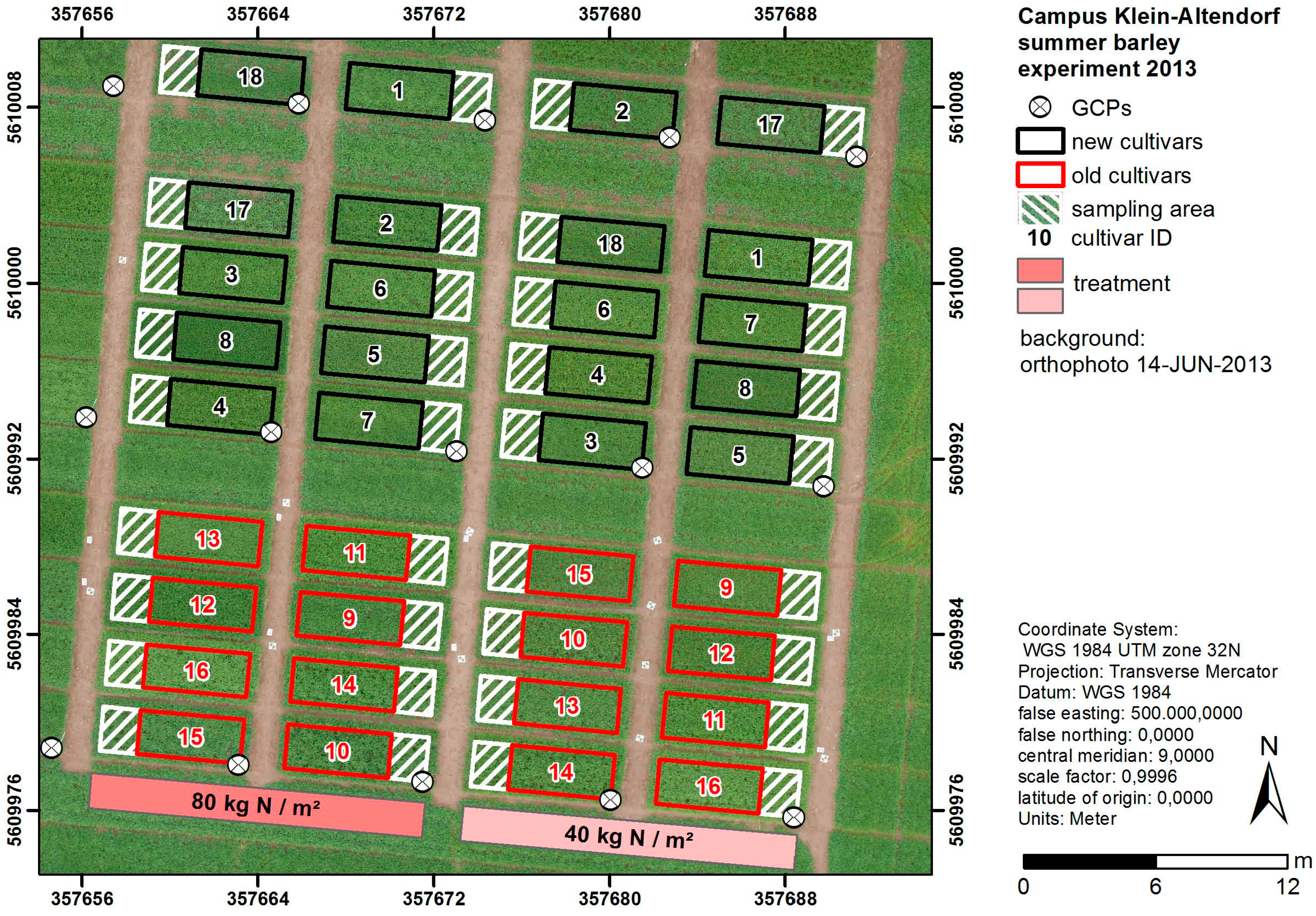
2.2. Biomass Sampling

| Type | Date | Number of Images Collected | BBCH *1 | Point Density (pt./m²) | Ø Image Overlap *2 |
|---|---|---|---|---|---|
| UAV (ground model) | 30 April 2013 | 216 | |||
| UAV | 14 May 2013 | 378 | 2878 | >9 | |
| Biomass | 14 May 2013 | tillering (21–27) | |||
| UAV | 28 May 2013 | 783 | 2675 | >9 | |
| Biomass | 28 May 2013 | tillering-stem elongation (25–35) | |||
| UAV | 14 June 2013 | 363 | 2958 | >9 | |
| Biomass | 12 June 2013 | booting (41–47) | |||
| UAV | 25 June 2013 | 300 | 3452 | >9 | |
| Biomass | 25 June 2013 | inflorescence emergence, heading (51–59) | |||
| UAV | 8 July 2013 | 342 | 2836 | >9 | |
| Biomass | 9 July 2013 | development of fruit (71–75) | |||
| UAV | 23 July 2013 | 265 | 2653 | >9 | |
| Biomass | 22 July 2013 | development of fruit-ripening (77–89) |
2.3. Platform
2.4. Sensor
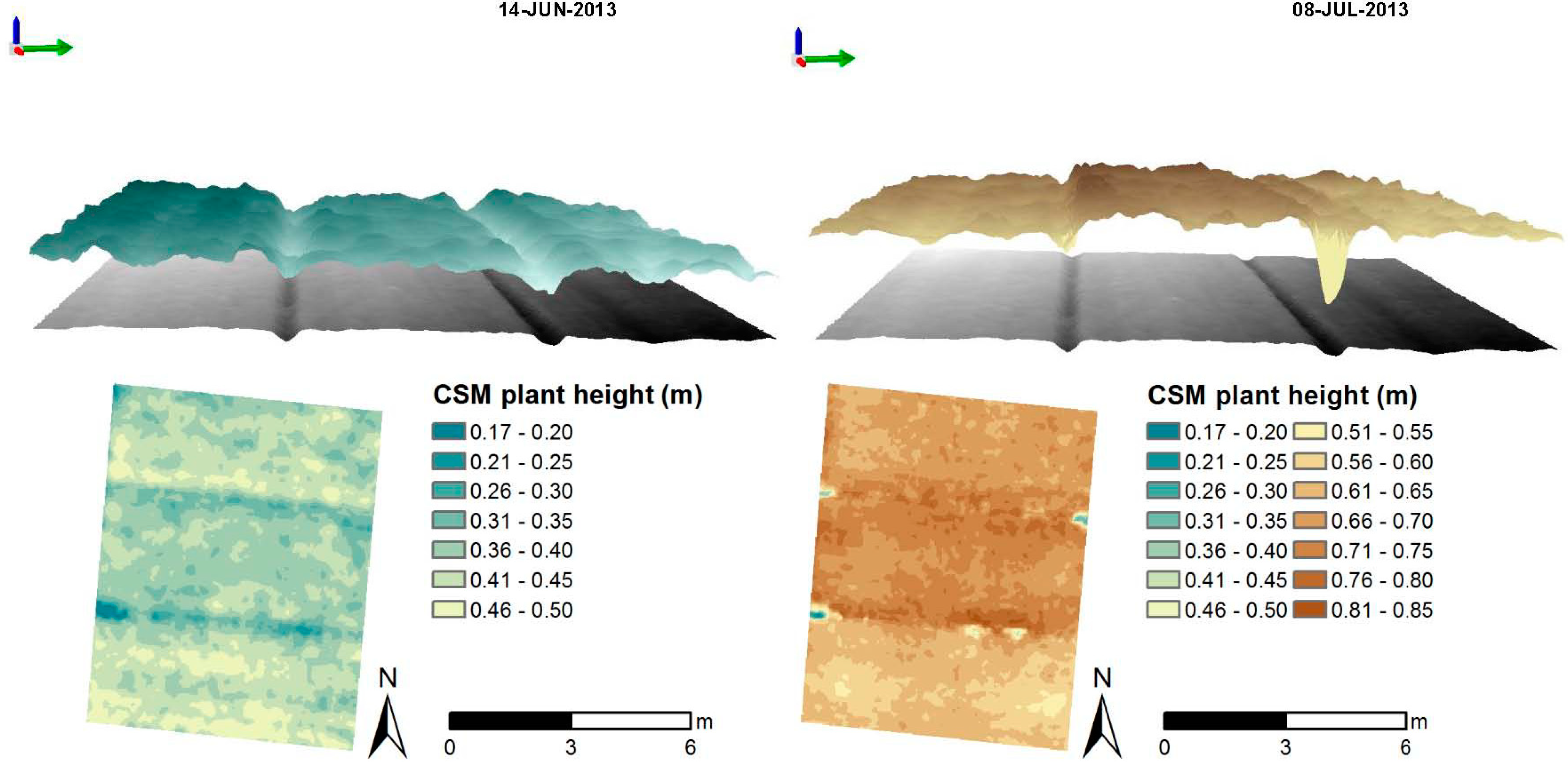
2.5. Generating CSMs
| PHref (m) | PHCSM (m) | Fresh Biomass (kg/m²) | Dry Biomass (kg/m²) | |
|---|---|---|---|---|
| Min | 0.14 | −0.03 | 0.22 | 0.03 |
| Max | 1.00 | 0.80 | 8.29 | 2.70 |
| Mean | 0.55 | 0.43 | 3.24 | 0.81 |
| SE | 0.25 | 0.25 | 1.96 | 0.68 |
| n | 216 | 216 | 216 | 216 |
2.6. Statistical Analyses
| R2 | PHref (m) | PHCSM (m) | Fresh Biomass (kg/m²) | Dry Biomass (kg/m²) |
|---|---|---|---|---|
| PHref (m) | 1 | |||
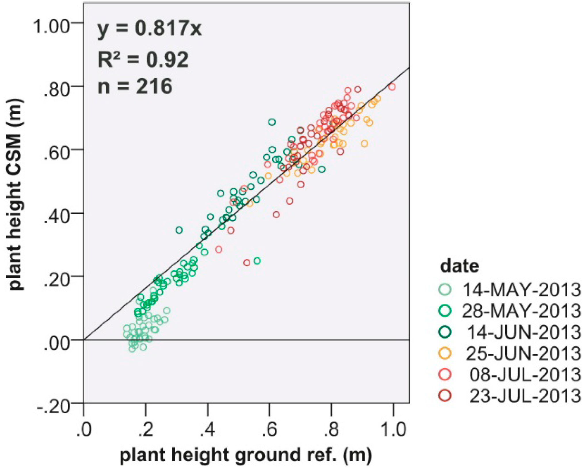
| PHCSM (m) | 0.92 (lin.) | 1 | ||
| fresh biomass (kg/m²) | 0.76 (exp.) | 0.81 (exp.) | 1 | |
| dry biomass (kg/m²) | 0.79 (exp.) | 0.82 (exp.) | 0.67 (lin.) | 1 |
3. Results
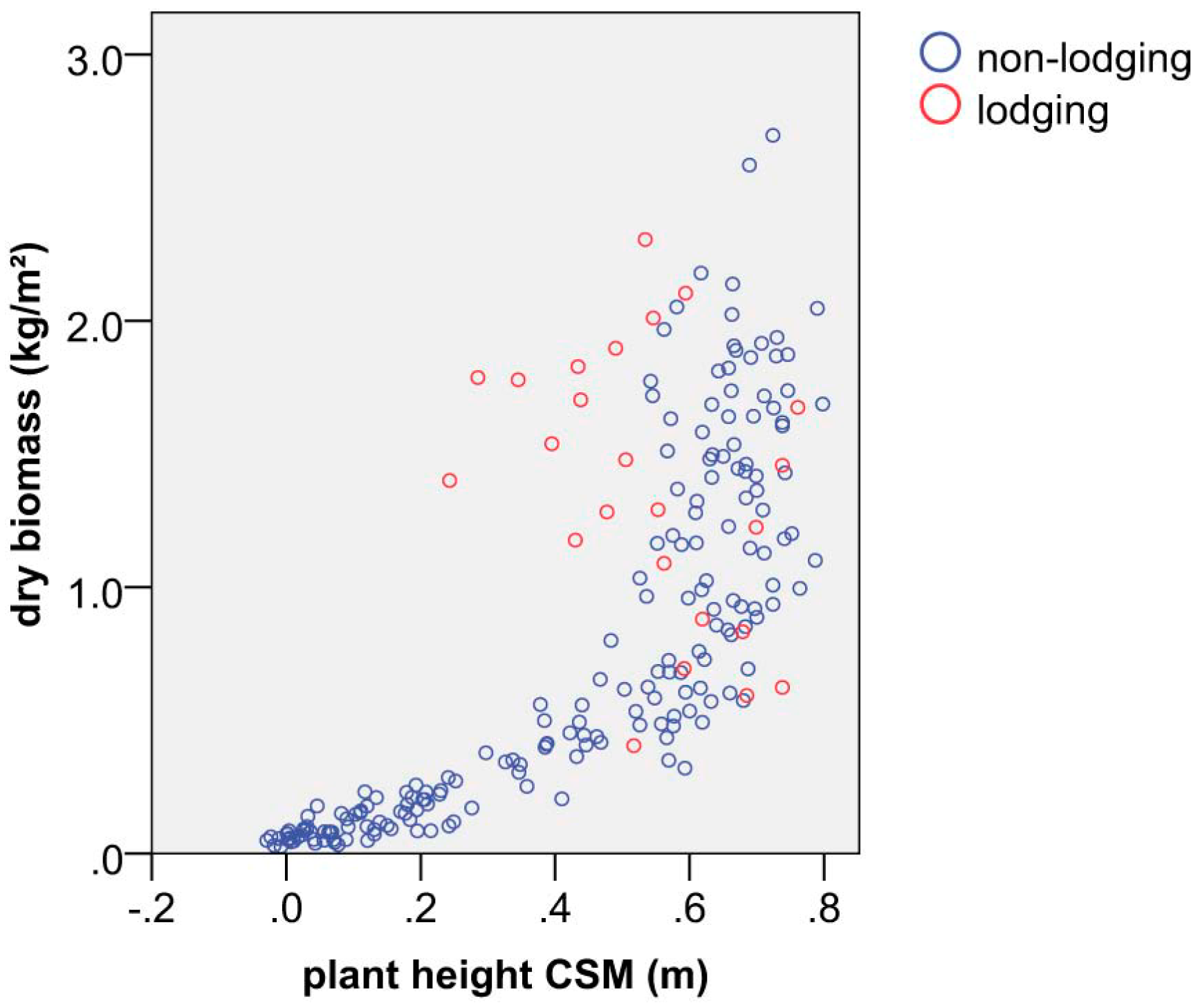
3.1. Plant Height and Biomass Samples
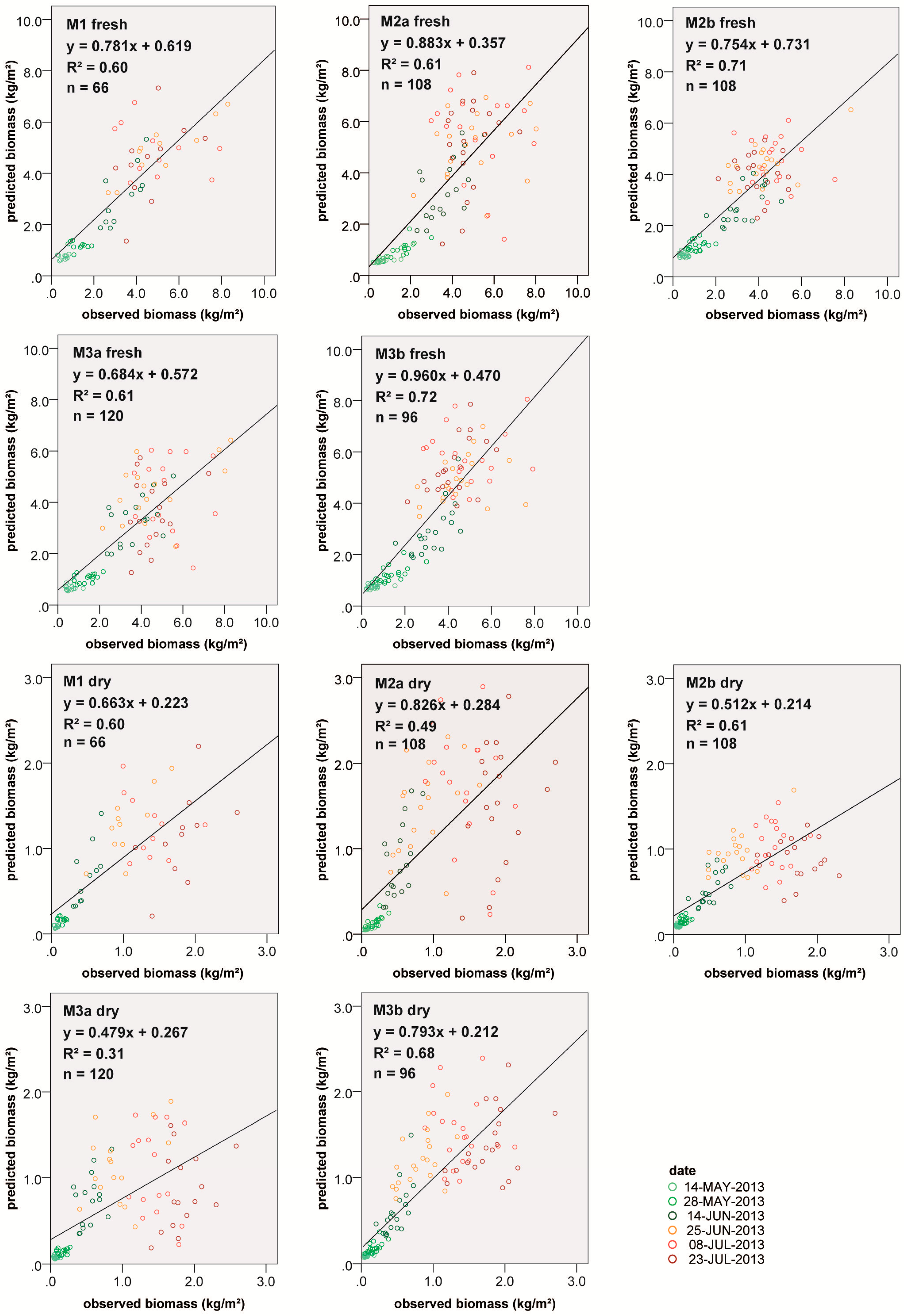
| Calibration/Validation Dataset | Regression Model | n | SE (kg/m2) | R2 | RMSE (kg/m2) | RE (%) |
|---|---|---|---|---|---|---|
| Fresh Biomass | ||||||
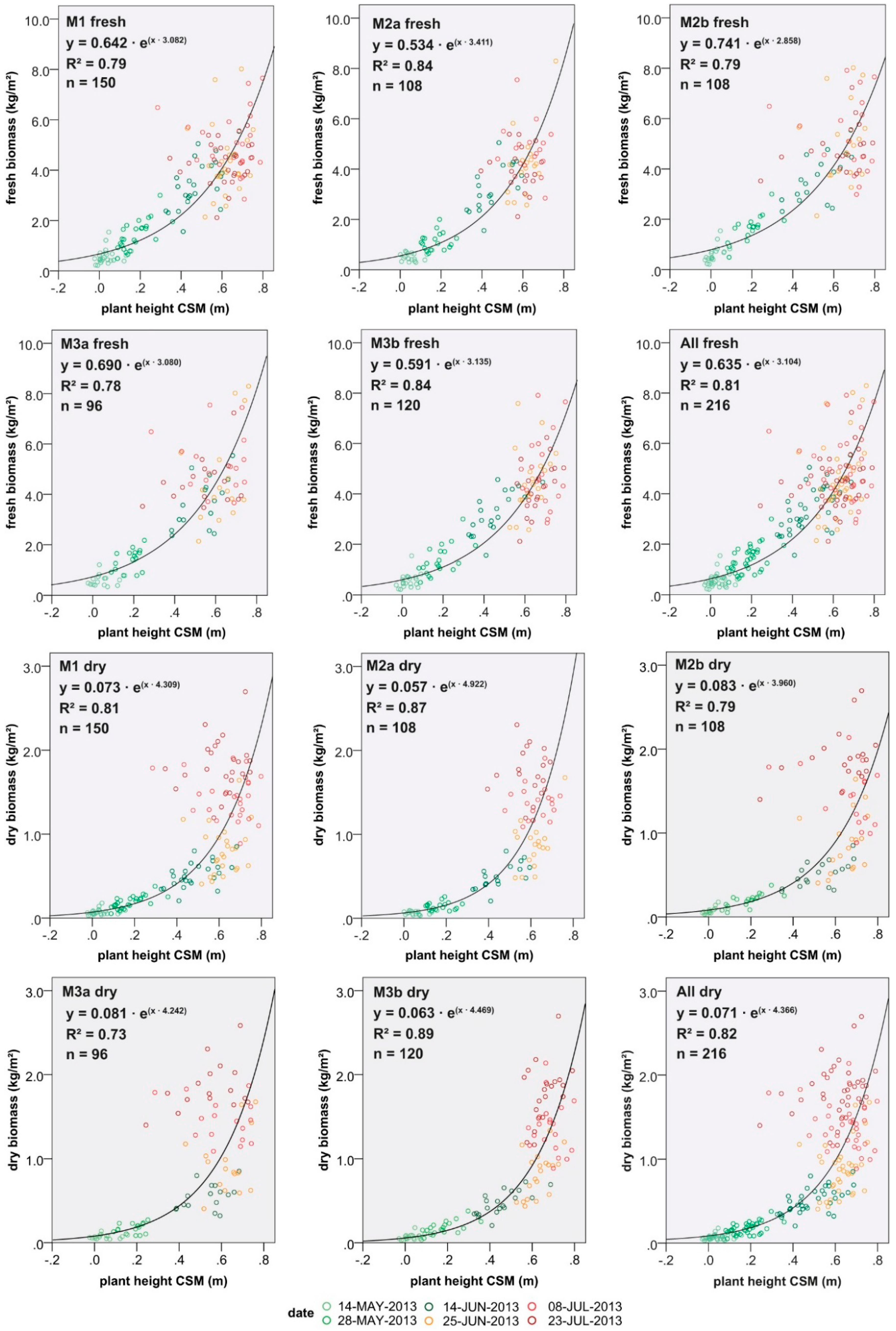
| M1: 70%/30% | BIOM = 0.642 × exp(PH × 3.082) | 66 | 3.21 | 0.71 | 1.95 | 60.87 |
| M2a: 40/80 kg N/m2 | BIOM = 0.534 × exp(PH × 3.411) | 108 | 3.46 | 0.61 | 2.35 | 67.72 |
| M2b: 80/40 kg N/m2 | BIOM = 0.741 × exp(PH × 2.858) | 108 | 2.97 | 0.71 | 1.60 | 54.04 |
| M3a: old/new cultivars | BIOM = 0.690 × exp(PH × 3.080) | 120 | 3.49 | 0.61 | 2.15 | 61.50 |
| M3b: new/old cultivars | BIOM = 0.591 × exp(PH × 3.135) | 96 | 2.87 | 0.72 | 1.77 | 61.79 |
| Dry Biomass | ||||||
| M1: 70%/30% | BIOM = 0.073 × exp(PH × 4.309) | 66 | 0.77 | 0.60 | 0.59 | 76.50 |
| M2a: 40/80 kg N/m2 | BIOM = 0.057 × exp(PH × 4.922) | 108 | 0.98 | 0.49 | 0.83 | 84.61 |
| M2b: 80/40 kg N/m2 | BIOM = 0.083 × exp(PH × 3.960) | 108 | 0.61 | 0.61 | 0.42 | 68.41 |
| M3a: old/new cultivars | BIOM = 0.081 × exp(PH × 4.242) | 120 | 0.67 | 0.39 | 0.54 | 79.88 |
| M3b: new/old cultivars | BIOM = 0.063 × exp(PH × 4.469) | 96 | 0.83 | 0.68 | 0.64 | 76.28 |
3.2. Biomass Modelling
3.2.1. Model Development
3.2.2. Model Application
4. Discussion
5. Conclusions and Outlook
Acknowledgments
Author Contributions
Conflicts of Interest
References and Notes
- Mulla, D.J. Twenty five years of remote sensing in precision agriculture: Key advances and remaining knowledge gaps. Biosyst. Eng. 2013, 114, 358–371. [Google Scholar]
- Laudien, R.; Bareth, G. Multitemporal hyperspectral data analysis for regional detection of plant diseases by using a tractor- and an airborne-based spectrometer. Photogramm. Fernerkund. Geoinf. 2006, 3, 217–227. [Google Scholar]
- Goyne, P.J.; Meinke, H.; Milroy, S.P.; Hammer, G.L.; Hare, J.M. Development and use of a barley crop simulation model to evaluate production management strategies in north-eastern Australia. Crop.Pasture Sci. 1996, 47, 997–1015. [Google Scholar]
- Shanahan, J.F.; Schepers, J.S.; Francis, D.D.; Varvel, G.E.; Wilhelm, W.W.; Tringe, J.M.; Schlemmer, M.R.; Major, D.J. Use of remote-sensing imagery to estimate corn grain yield. Agron. J. 2001, 93, 583–589. [Google Scholar]
- Adamchuk, V.I.; Ferguson, R.B.; Hergert, G.W. Soil heterogeneity and crop growth. In Precision Crop Protection—The Challenge and Use of Heterogeneity; Oerke, E.-C., Gerhards, R., Menz, G., Sikora, R.A., Eds.; Springer: Dordrecht, The Netherlands, 2010; pp. 3–16. [Google Scholar]
- Thenkabail, P.S.; Smith, R.B.; De Pauw, E. Hyperspectral vegetation indices and their relationships with agricultural crop characteristics. Remote Sens. Environ. 2000, 71, 158–182. [Google Scholar]
- Jensen, A.; Lorenzen, B.; Østergaard, H.S.; Hvelplund, E.K. Radiometric estimation of biomass and nitrogen content of barley grown at different nitrogen levels. Int. J. Remote Sens. 1990, 11, 1809–1820. [Google Scholar]
- Chen, P.; Haboudane, D.; Tremblay, N.; Wang, J.; Vigneault, P.; Li, B. New spectral indicator assessing the efficiency of crop nitrogen treatment in corn and wheat. Remote Sens. Environ. 2010, 114, 1987–1997. [Google Scholar]
- Lemaire, G.; Gastal, F. N uptake and distribution in plant canopies. In Diagnosis of the Nitrogen Status in Crops; Lemaire, D.G., Ed.; Springer: Berlin, Germany, 1997; pp. 3–43. [Google Scholar]
- Lemaire, G.; Jeuffroy, M.-H.; Gastal, F. Diagnosis tool for plant and crop N status in vegetative stage. Eur. J. Agron. 2008, 28, 614–624. [Google Scholar]
- Kumar, L.; Schmidt, K.; Dury, S.; Skidmore, A. Imaging spectrometry and vegetation science. In Imaging Spectrometry; Van der Meer, F.D., Jong, S.M.D., Eds.; Kluwer Academic Publishers: Dordrecht, The Netherlands, 2001; pp. 111–155. [Google Scholar]
- Koppe, W.; Gnyp, M.L.; Hennig, S.D.; Li, F.; Miao, Y.; Chen, X.; Jia, L.; Bareth, G. Multi-temporal hyperspectral and radar remote sensing for estimating winter wheat biomass in the North China Plain. Photogramm. Fernerkund. Geoinf. 2012, 3, 281–298. [Google Scholar]
- Migdall, S.; Bach, H.; Bobert, J.; Wehrhan, M.; Mauser, W. Inversion of a canopy reflectance model using hyperspectral imagery for monitoring wheat growth and estimating yield. Precis. Agric. 2009, 10, 508–524. [Google Scholar]
- Yang, C.; Everitt, J.H.; Bradford, J.M. Yield estimation from hyperspectral imagery using spectral angle mapper (SAM). Trans. ASABE 2008, 51, 729–737. [Google Scholar]
- Jang, G.-S.; Sudduth, K.A.; Hong, S.Y.; Kitchen, N.R.; Palm, H.L. Relating hyperspectral image bands and vegetation indices to corn and soybean yield. Korean J. Remote Sens. 2006, 22, 183–197. [Google Scholar]
- Hoyos-Villegas, V.; Fritschi, F.B. Relationships among vegetation indices derived from aerial photographs and soybean growth and yield. Crop Sci. 2013, 53, 2631–2642. [Google Scholar]
- Sakamoto, T.; Gitelson, A.A.; Nguy-Robertson, A.L.; Arkebauer, T.J.; Wardlow, B.D.; Suyker, A.E.; Verma, S.B.; Shibayama, M. An alternative method using digital cameras for continuous monitoring of crop status. Agric. For. Meteorol. 2012, 154–155, 113–126. [Google Scholar]
- Gnyp, M.L.; Bareth, G.; Li, F.; Lenz-Wiedemann, V.I.S.; Koppe, W.; Miao, Y.; Hennig, S.D.; Jia, L.; Laudien, R.; Chen, X.; et al. Development and implementation of a multiscale biomass model using hyperspectral vegetation indices for winter wheat in the North China Plain. Int. J. Appl. Earth Obs. Geoinf. 2014, 33, 232–242. [Google Scholar]
- Li, F.; Miao, Y.; Hennig, S.D.; Gnyp, M.L.; Chen, X.; Jia, L.; Bareth, G. Evaluating hyperspectral vegetation indices for estimating nitrogen concentration of winter wheat at different growth stages. Precis. Agric. 2010, 11, 335–357. [Google Scholar]
- Lati, R.N.; Filin, S.; Eizenberg, H. Estimating plant growth parameters using an energy minimization-based stereovision model. Comput. Electron. Agric. 2013, 98, 260–271. [Google Scholar]
- Bendig, J.; Bolten, A.; Bareth, G. UAV-based imagzing for multi-temporal, very high resolution crop surface models to monitor crop growth variability. Photogramm. Fernerkund. Geoinf. 2013, 6, 551–562. [Google Scholar]
- Hoffmeister, D.; Bolten, A.; Curdt, C.; Waldhoff, G.; Bareth, G. High-resolution Crop Surface Models (CSM) and Crop Volume Models (CVM) on field level by terrestrial laser scanning. Proc. SPIE 2010, 7840. [Google Scholar] [CrossRef]
- Hoffmeister, D.; Waldhoff, G.; Curdt, C.; Tilly, N.; Bendig, J.; Bareth, G. Spatial variability detection of crop height in a single field by terrestrial laser scanning. In Precision Agriculture’13; Stafford, J.V., Ed.; Wageningen Academic Publishers: Lleida, Spain, 2013; pp. 267–274. [Google Scholar]
- Tilly, N.; Hoffmeister, D.; Cao, Q.; Huang, S.; Lenz-Wiedemann, V.I.S.; Miao, Y.; Bareth, G. Multitemporal crop surface models: Accurate plant height measurement and biomass estimation with terrestrial laser scanning in paddy rice. J. Appl. Remote Sens. 2014, 8, 083671–083671. [Google Scholar]
- Tilly, N.; Hoffmeister, D.; Liang, H.; Cao, Q.; Liu, Y.; Lenz-Wiedemann, V.; Miao, Y.; Bareth, G. Evaluation of terrestrial laser scanning for rice growth monitoring. Int.Arch. Photogramm. Remote Sens. Spat. Inf. Sci. 2012, XXXIX-B7, 351–356. [Google Scholar]
- Hoffmeister, D.; Curdt, C.; Tilly, N.; Bendig, J.; Bareth, G. 3D change detection of different sugar-beet types by multi-temporal terrestrial laser scanning. In Proceedings of 2011 International Symposium on Remote Sensing and GIS Methods for Change Detection and Spatio-Temporal Modelling (CDSM), Hong Kong, China, 15–16 December 2011; p. 5.
- Lumme, J.; Karjalainen, M.; Kaartinen, H.; Kukko, A.; Hyyppä, J.; Hyyppä, H.; Jaakkola, A.; Kleemola, J. Terrestrial laser scanning of agricultural crops. Int. Arch. Photogramm. Remote Sens. Spat. Inf. Sci. 2008, 37, 563–566. [Google Scholar]
- Ehlert, D.; Adamek, R.; Horn, H.-J. Laser rangefinder-based measuring of crop biomass under field conditions. Precis. Agric. 2009, 10, 395–408. [Google Scholar]
- Colomina, I.; Molina, P. Unmanned aerial systems for photogrammetry and remote sensing: A review. ISPRS J. Photogramm. Remote Sens. 2014, 92, 79–97. [Google Scholar]
- Zarco-Tejada, P.J. A new era in remote sensing of crops with unmanned robots. Proc. SPIE 2008, 7480, 2–4. [Google Scholar]
- Jensen, T.; Apan, A.; Young, F.; Zeller, L. Detecting the attributes of a wheat crop using digital imagery acquired from a low-altitude platform. Comput. Electron. Agric. 2007, 59, 66–77. [Google Scholar] [Green Version]
- Hunt, E.R.; Hively, W.D.; McCarty, G.W.; Daughtry, C.S.T.; Forrestal, P.J.; Kratochvil, R.J.; Carr, J.L.; Allen, N.F.; Fox-Rabinovitz, J.R.; Miller, C.D. NIR-green-blue high-resolution digital images for assessment of winter cover crop biomass. GISci. Remote Sens. 2011, 48, 86–98. [Google Scholar]
- Agüera, F.; Carvajal, F.; Pérez, M. Measuring sun-flower nitrogen status from an unmanned aerial vehicle-based system and an on the ground device. Int. Arch. Photogramm. Remote Sens. Spat. Inf. Sci. 2011, 38, 33–37. [Google Scholar]
- Berni, J.A.J.; Zarco-Tejada, P.J.; Suárez, L.; González-Dugo, V.; Fereres, E. Remote sensing of vegetation from UAV platforms using lightweight multispectral and thermal imaging sensors. Int. Arch. Photogramm. Remote Sens. Spat. Inf. Sci. 2009, 38, 6. [Google Scholar]
- Baluja, J. Assessment of vineyard water status variability by thermal and multispectral imagery using an Unmanned Aerial Vehicle (UAV). Irrig. Sci. 2012, 6, 511–522. [Google Scholar]
- Turner, D.; Lucieer, A.; Malenovský, Z.; King, D.; Robinson, S. Spatial co-registration of ultra-high resolution visible, multispectral and thermal images acquired with a micro-UAV over Antarctic Moss Beds. Remote Sens. 2014, 6, 4003–4024. [Google Scholar]
- Verhoeven, G. Taking computer vision aloft—Archaeological three-dimensional reconstructions from aerial photographs with photoscan. Archaeol. Prospect. 2011, 18, 67–73. [Google Scholar]
- Turner, D.; Lucieer, A.; Watson, C. An automated technique for generating georectified mosaics from ultra-high resolution unmanned aerial vehicle (UAV) imagery, based on structure from motion (SfM) point clouds. Remote Sens. 2012, 4, 1392–1410. [Google Scholar]
- Lucieer, A.; Turner, D.; King, D.H.; Robinson, S.A. Using an Unmanned Aerial Vehicle (UAV) to capture micro-topography of Antarctic moss beds. Int. J. Appl. Earth Obs. Geoinf. 2014, 27, 53–62. [Google Scholar]
- Baiocchi, V.; Dominici, D.; Elaiopoulos, M.; Massimi, V.; Mormile, M.; Rosciano, E. UAV flight plan software: first implementation of UP23d. In Proceedings of 2013 EARSeL Symposium Towards Horizon 2020: Earth Observation and Social Perspectives, Matera, Italy, 3–6 June 2013; pp. 829–841.
- Ehlert, D.; Horn, H.-J.; Adamek, R. Measuring crop biomass density by laser triangulation. Comput. Electron. Agric. 2008, 61, 117–125. [Google Scholar]
- Busemeyer, L.; Mentrup, D.; Möller, K.; Wunder, E.; Alheit, K.; Hahn, V.; Maurer, H.P.; Reif, J.C.; Würschum, T.; Müller, J.; et al. Breedvision—A multi-sensor platform for non-destructive field-based phenotyping in plant breeding. Sensors 2013, 13, 2830–2847. [Google Scholar]
- Grenzdörffer, G.; Zacharias, P. Bestandeshöhenermittlung landwirtschaftlicher Kulturen aus UAS-Punktwolken. DGPF Tagungsband 2014, 23, 1–8. [Google Scholar]
- Scotford, I.M.; Miller, P.C.H. Combination of spectral reflectance and ultrasonic sensing to monitor the growth of winter wheat. Biosyst.Eng. 2004, 87, 27–38. [Google Scholar]
- Clevers, J.P.G.W.; Jongschaap, R. Imaging spectrometry for agricultural applications. In Imaging Spectrometry; Van der Meer, F.D., Jong, S.M.D., Eds.; Kluwer Academic Publishers: Dordrecht, The Netherlands, 2001; pp. 157–199. [Google Scholar]
- Confalonieri, R.; Bregaglio, S.; Rosenmund, A.S.; Acutis, M.; Savin, I. A model for simulating the height of rice plants. Eur. J. Agron. 2011, 34, 20–25. [Google Scholar]
- Doneus, M.; Verhoeven, G.; Fera, M.; Briese, C.; Kucera, M.; Neubauer, W. From deposit to point cloud: a study of low-cost computer vision approaches for the straightforward documentation of archaeological excavations. In Proceedings of 2011 International CIPA Symposium, Prague, Czech Republic, 12–16 September 2011; pp. 81–88.
- Naumann, M.; Bill, R.; Niemeyer, F.; Nitschke, E. Deformation analysis of dikes using Unmanned Aerial Systems (UAS). In Proceedings of the South Baltic Conference on Dredged Materials in Dike Construction, Rostock, Germany, 10–12 April 2014; pp. 119–126.
- Niethammer, U.; James, M.R.; Rothmund, S.; Travelletti, J.; Joswig, M. UAV-based remote sensing of the Super-Sauze landslide: Evaluation and results. Eng. Geol. 2012, 128, 2–11. [Google Scholar]
- Höfle, B. Radiometric correction of terrestrial LiDAR point cloud data for individual maize plant detection. IEEE Geosci. Remote Sens. Lett. 2014, 1, 94–98. [Google Scholar]
- Swain, K.C.; Thomson, S.J.; Jayasuriya, H.P.W. Adoption of an unmanned helicopter for low-altitude remote sensing to estimate yield and total biomass of a rice crop. Trans. ASAE 2010, 53, 21–27. [Google Scholar]
- Eling, C.; Klingbeil, L.; Wieland, M.; Kuhlmann, H. A precise position and attitude determination system for lighweight unmanned aerial vehicles. Int. Arch. Photogramm. Remote Sens. Spat. Inf. Sci. 2013, XL-1/W2, 113–118. [Google Scholar]
- Turner, D.; Lucieer, A.; Wallace, L. Direct georeferencing of ultrahigh-resolution UAV imagery. IEEE Trans. Geosci. Remote Sens. 2014, 52, 2738–2745. [Google Scholar]
- Pfeifer, N.; Glira, P.; Briese, C. Direct georeferencing with on board navigation components of light weight UAV platforms. Int. Arch. Photogramm. RemoteSens. Spat. Inf. Sci. 2012, XXXIX-B7, 487–492. [Google Scholar]
- Eling, C.; Klingbeil, L.; Wieland, M.; Kuhlmann, H. Direct georeferencing of micro aerial vehicles—System design, system calibration and first evaluation tests. Photogramm. Fernerkund. Geoinf. 2014, 4, 227–237. [Google Scholar]
- Yu, K.; Lenz-Wiedemann, V.; Leufen, G.; Hunsche, M.; Noga, G.; Chen, X.; Bareth, G. Assessing hyperspectral vegetation indices for estimating leaf chlorophyll concentration of summer barley. ISPRS Ann. Photogramm. Remote Sens. Spat. Inf. Sci. 2012, I-7, 89–94. [Google Scholar]
- Bareth, G.; Bendig, J.; Aasen, H.; Gnyp, M.L.; Bolten, A.; Jung, A.; Michels, R.; Soukkamäki, J. Low-weight and UAV-based hyperspectral full-frame cameras for monitoring crops: Spectral comparison with portable spectroradiometer measurements. Photogramm. Fernerkund. Geoinf. 2015, in press. [Google Scholar]
- Honkavaara, E.; Saari, H.; Kaivosoja, J.; Pölönen, I.; Hakala, T.; Litkey, P.; Mäkynen, J.; Pesonen, L. Processing and assessment of spectrometric, stereoscopic imagery collected using a lightweight UAV spectral camera for precision agriculture. Remote Sens. 2013, 5, 5006–5039. [Google Scholar]
- Hunt, E.R., Jr.; Cavigelli, M.; Daughtry, C.S.T.; Mcmurtrey, J.E., III; Walthall, C.L. Evaluation of digital photography from model aircraft for remote sensing of crop biomass and nitrogen status. Precis. Agric. 2005, 6, 359–378. [Google Scholar]
- Hunt, E.R., Jr.; Doraiswamy, P.C.; McMurtrey, J.E.; Daughtry, C.S.T.; Perry, E.M.; Akhmedov, B. A visible band index for remote sensing leaf chlorophyll content at the canopy scale. Int. J. Appl. Earth Obs. Geoinf. 2013, 21, 103–112. [Google Scholar]
© 2014 by the authors; licensee MDPI, Basel, Switzerland. This article is an open access article distributed under the terms and conditions of the Creative Commons Attribution license (http://creativecommons.org/licenses/by/4.0/).
Share and Cite
Bendig, J.; Bolten, A.; Bennertz, S.; Broscheit, J.; Eichfuss, S.; Bareth, G. Estimating Biomass of Barley Using Crop Surface Models (CSMs) Derived from UAV-Based RGB Imaging. Remote Sens. 2014, 6, 10395-10412. https://doi.org/10.3390/rs61110395
Bendig J, Bolten A, Bennertz S, Broscheit J, Eichfuss S, Bareth G. Estimating Biomass of Barley Using Crop Surface Models (CSMs) Derived from UAV-Based RGB Imaging. Remote Sensing. 2014; 6(11):10395-10412. https://doi.org/10.3390/rs61110395
Chicago/Turabian StyleBendig, Juliane, Andreas Bolten, Simon Bennertz, Janis Broscheit, Silas Eichfuss, and Georg Bareth. 2014. "Estimating Biomass of Barley Using Crop Surface Models (CSMs) Derived from UAV-Based RGB Imaging" Remote Sensing 6, no. 11: 10395-10412. https://doi.org/10.3390/rs61110395