Temporal Polarimetric Behavior of Oilseed Rape (Brassica napus L.) at C-Band for Early Season Sowing Date Monitoring


 ,
,  ,
,
Abstract
:1. Background and Rationale
2. Objectives
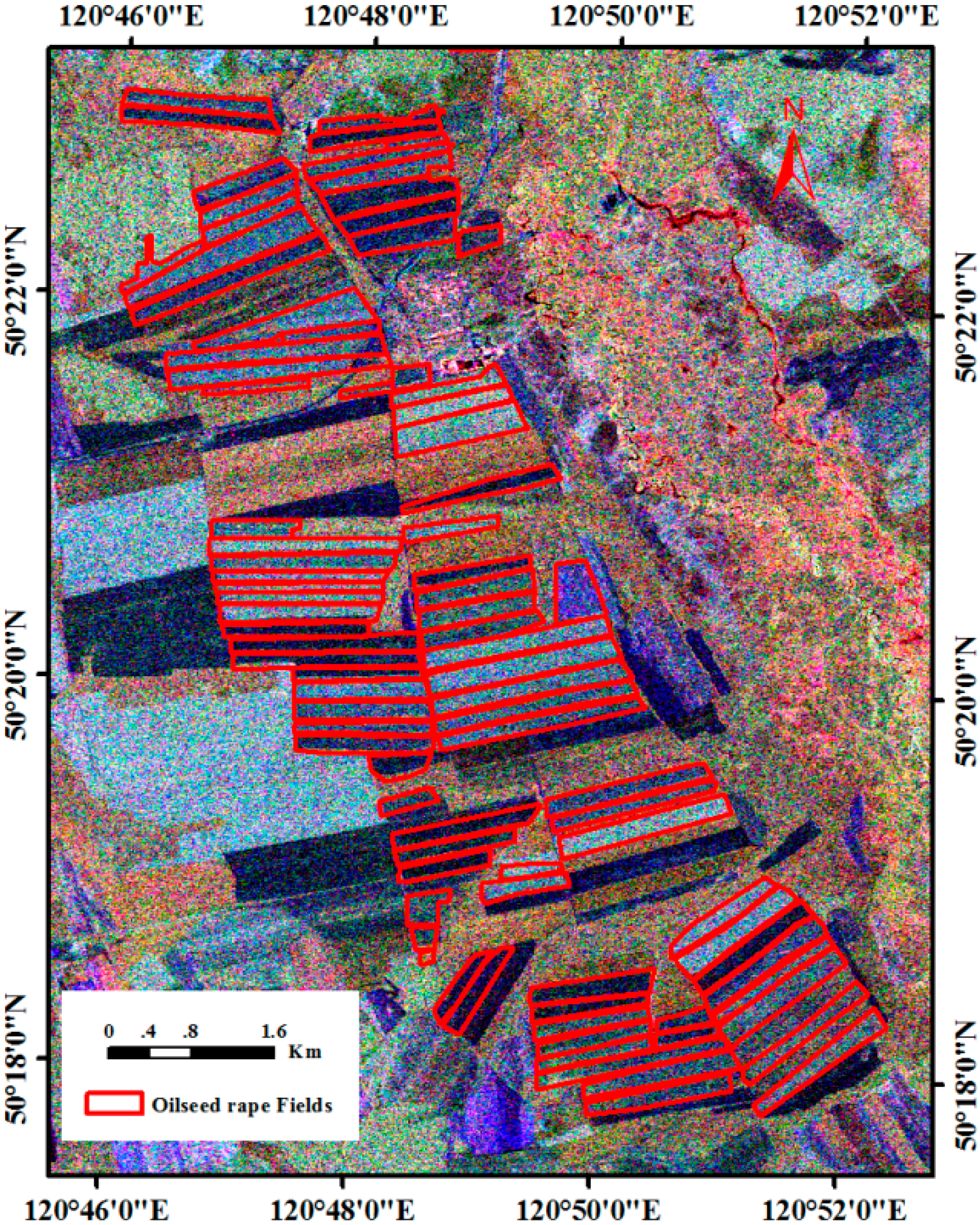
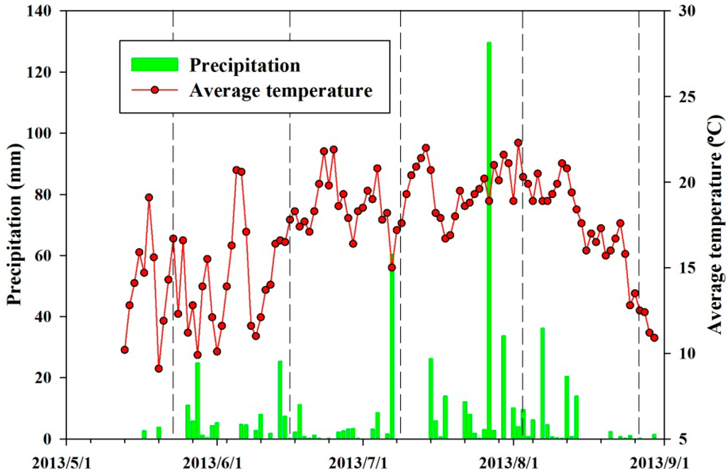
3. Study Area
4. Approach and Methods

| Parameter | Values |
|---|---|
| Imaging Mode | Fine Quad Polarization |
| Center frequency | 5.405 GHz |
| Incidence angle | 37.4°–38.8° |
| Resolution | about 8m |
| Orbit direction | Ascending |
| Beam mode | FQ18 |
| Acquired Time | UTC 09:47:33 |
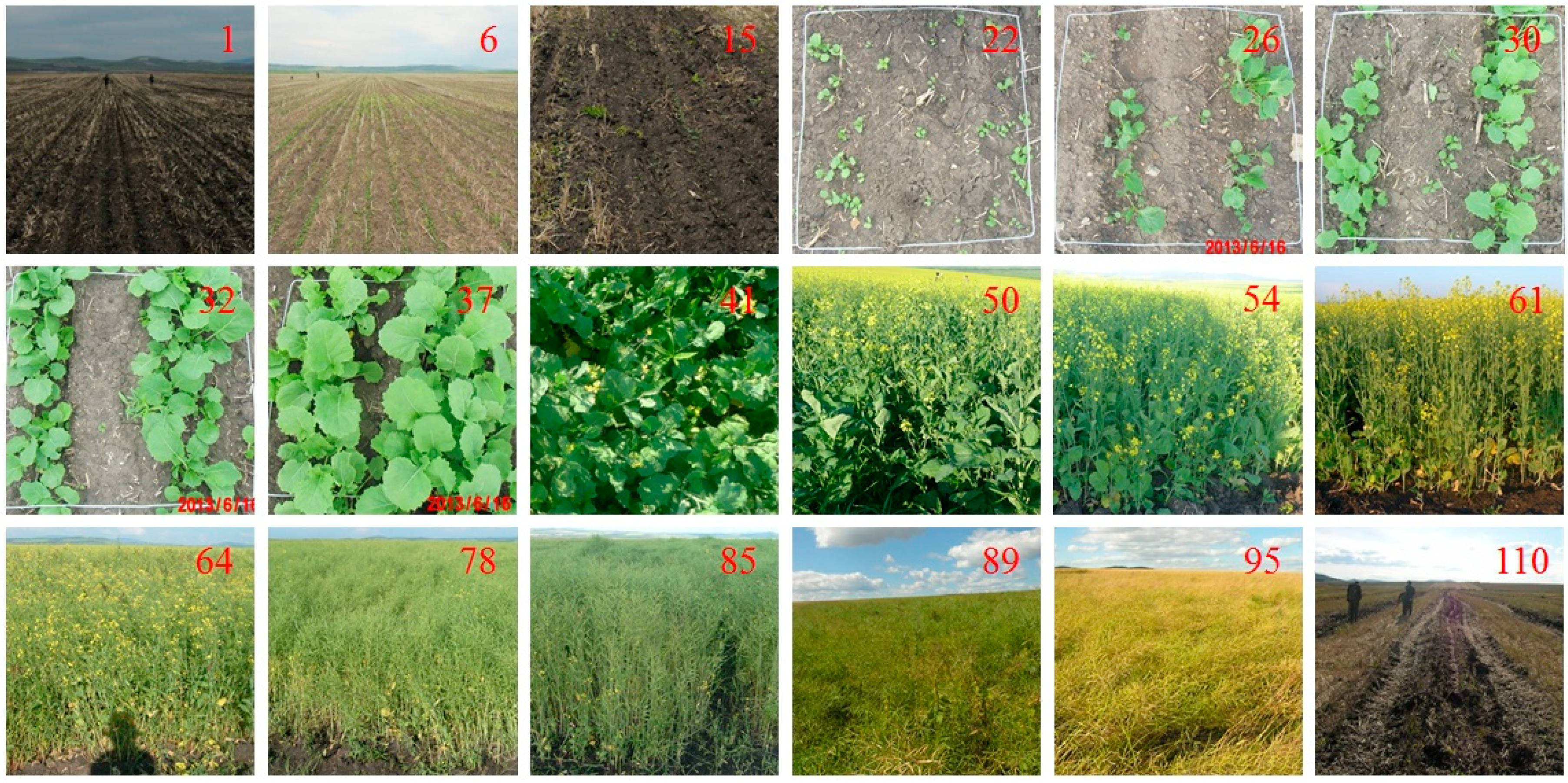
| Acquisition Dates | Principal Growth Stage [31] |
|---|---|
| 23 May 2013 | Germination (0) |
| 16 June 2013 | Leaf development (1) and formation of side shoots (2) |
| 10 July 2013 | Stem elongation (3), inflorescence emergence (5), and flowering (6) |
| 03 August 2013 | development of fruit (7) |
| 27 August 2013 | Ripening (8) and senescence (9) |

| Date | Number of Fields | DAS | LAI (m2/m2) | Soil Moisture (%) | Dry Biomass (g/m2) | PWC (g/g) |
|---|---|---|---|---|---|---|
| 23 May 2013 | 14 | [−7, 15] | - | [19.2, 42.4] | - | - |
| 32.7 | ||||||
| 16 June 2013 | 11 | [16, 39] | [0, 1.5] | [32.5, 43.8] | [9.5, 89.0] | [0.88, 0.92] |
| 0.6 | 37.8 | 37.7 | 0.90 | |||
| 10 July 2013 | 12 | [40, 63] | [2.5, 3.6] | [34.1, 47.4] | [86.8, 350.9] | [0.86, 0.94] |
| 3.1 | 41.7 | 207.3 | 0.90 | |||
| 03 August 2013 | 14 | [64, 87] | [2.2, 3.5] | [41.0, 59.8] | [694.7, 2009.2] | [0.81, 0.86] |
| 2.9 | 56.3 | 1210.4 | 0.84 | |||
| 27 August 2013 | 11 | [89, 110] | - | [22.4, 51.0] | [875.0, 2509.7] | [0.38, 0.75] |
| 41.3 | 1616.4 | 0.46 |

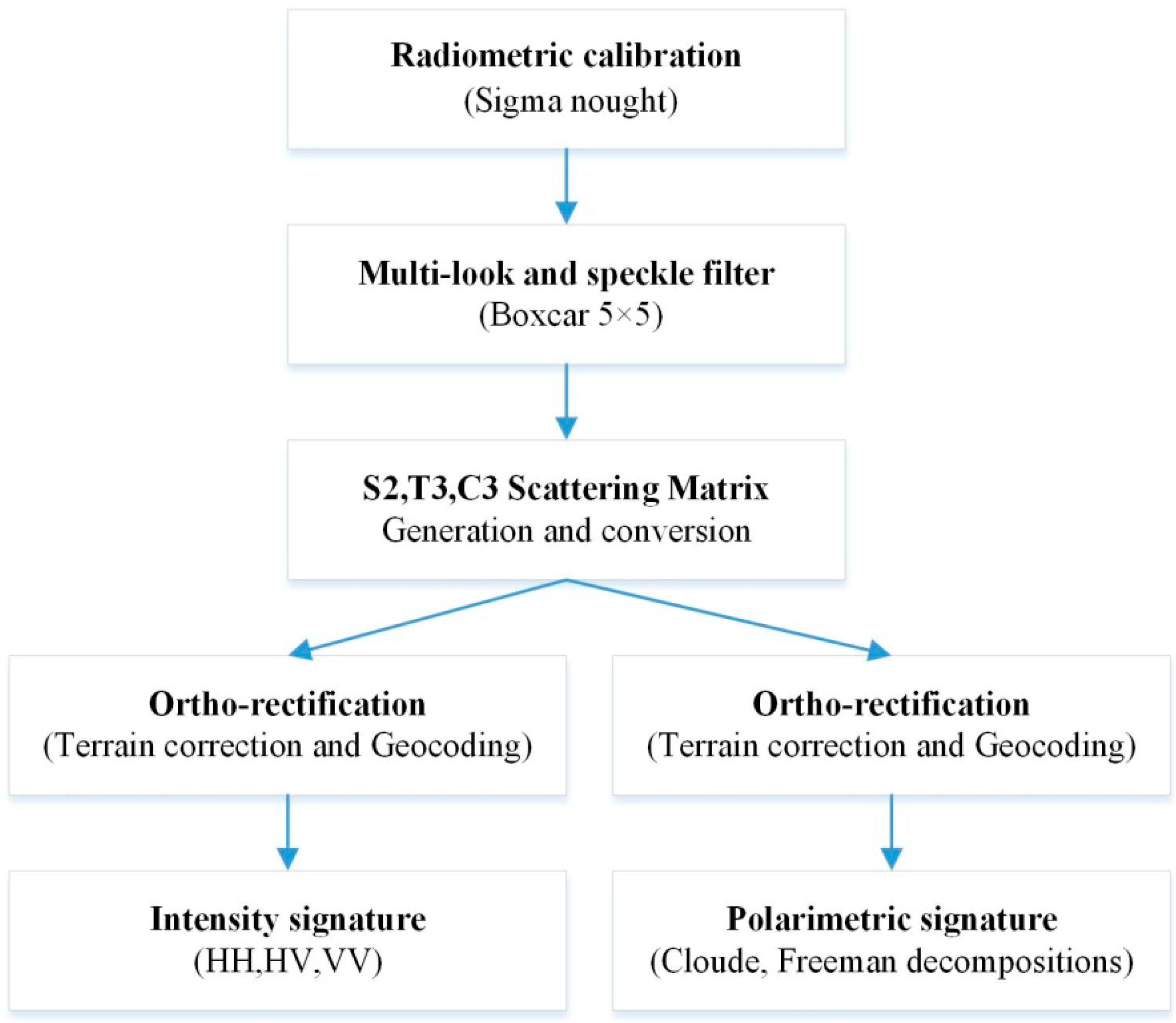
4.1. Preprocessing of SAR Image
4.2. Derivation of the Polarimetric Parameters
4.3. Analysis of the Temporal Evolution of Polarimetric Parameters and the Retrieval of the Sowing Dates
5. Results and Discussion
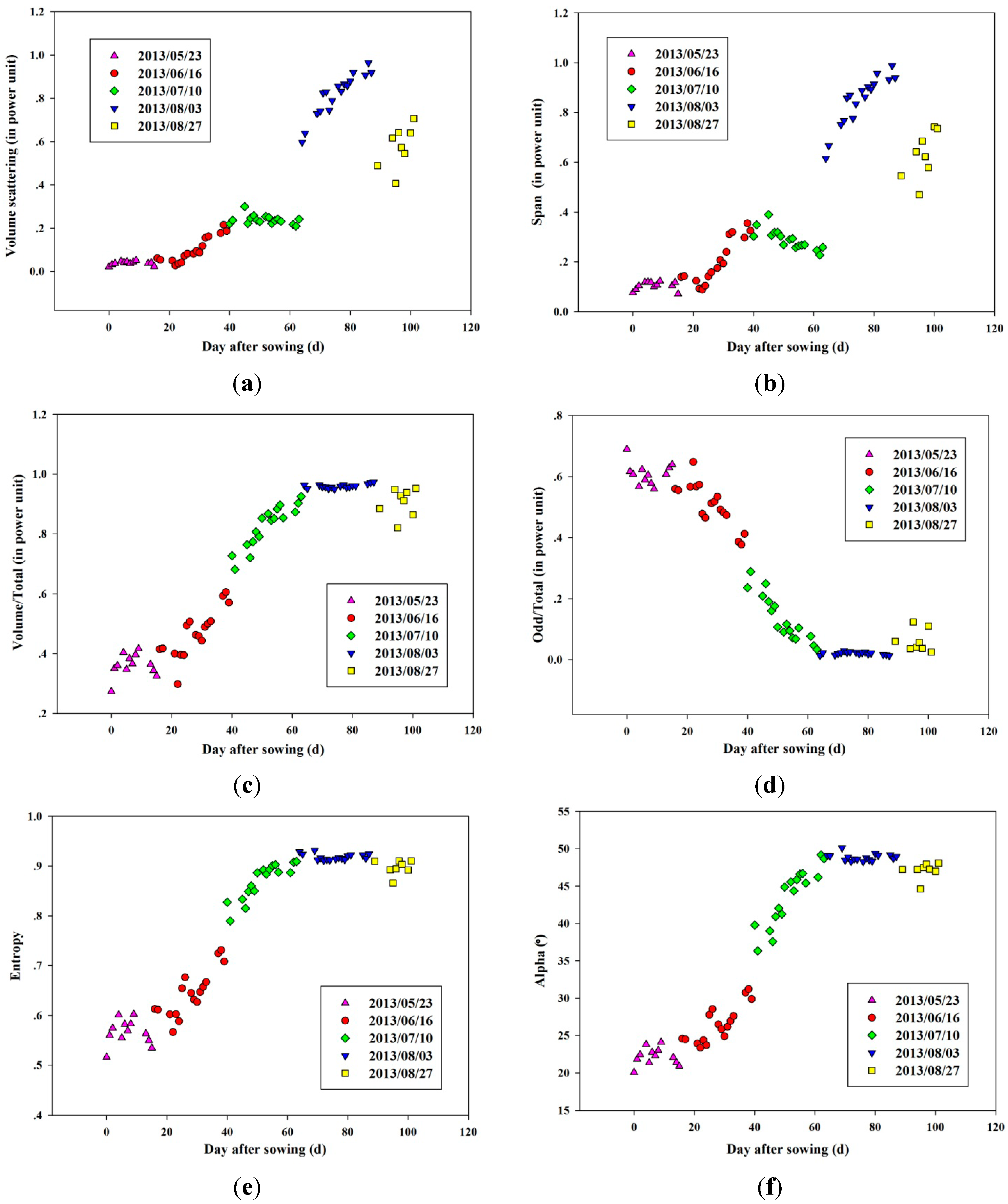
5.1. Temporal Behavior of the Polarimetric Response during the Crop Growing Season
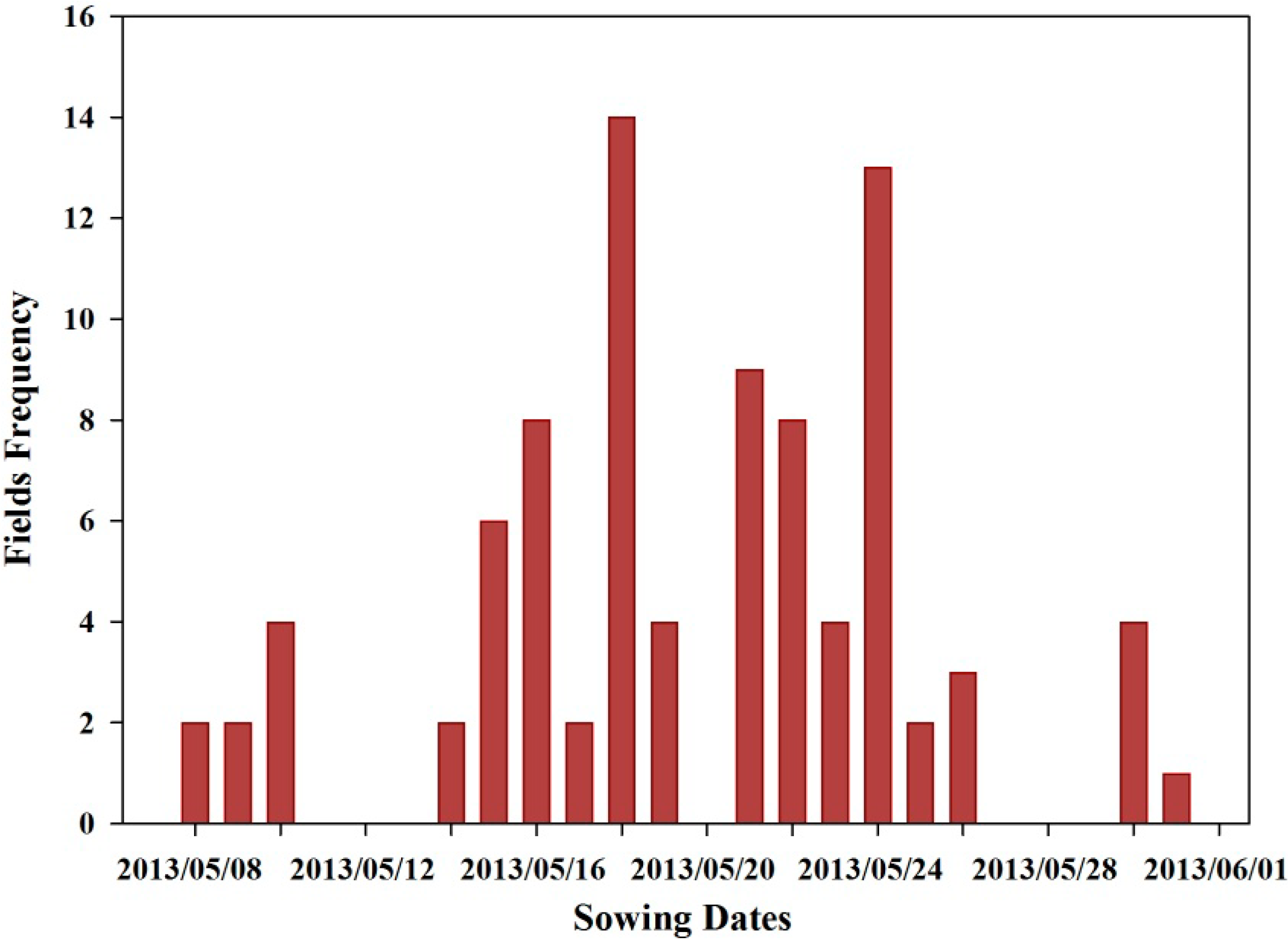
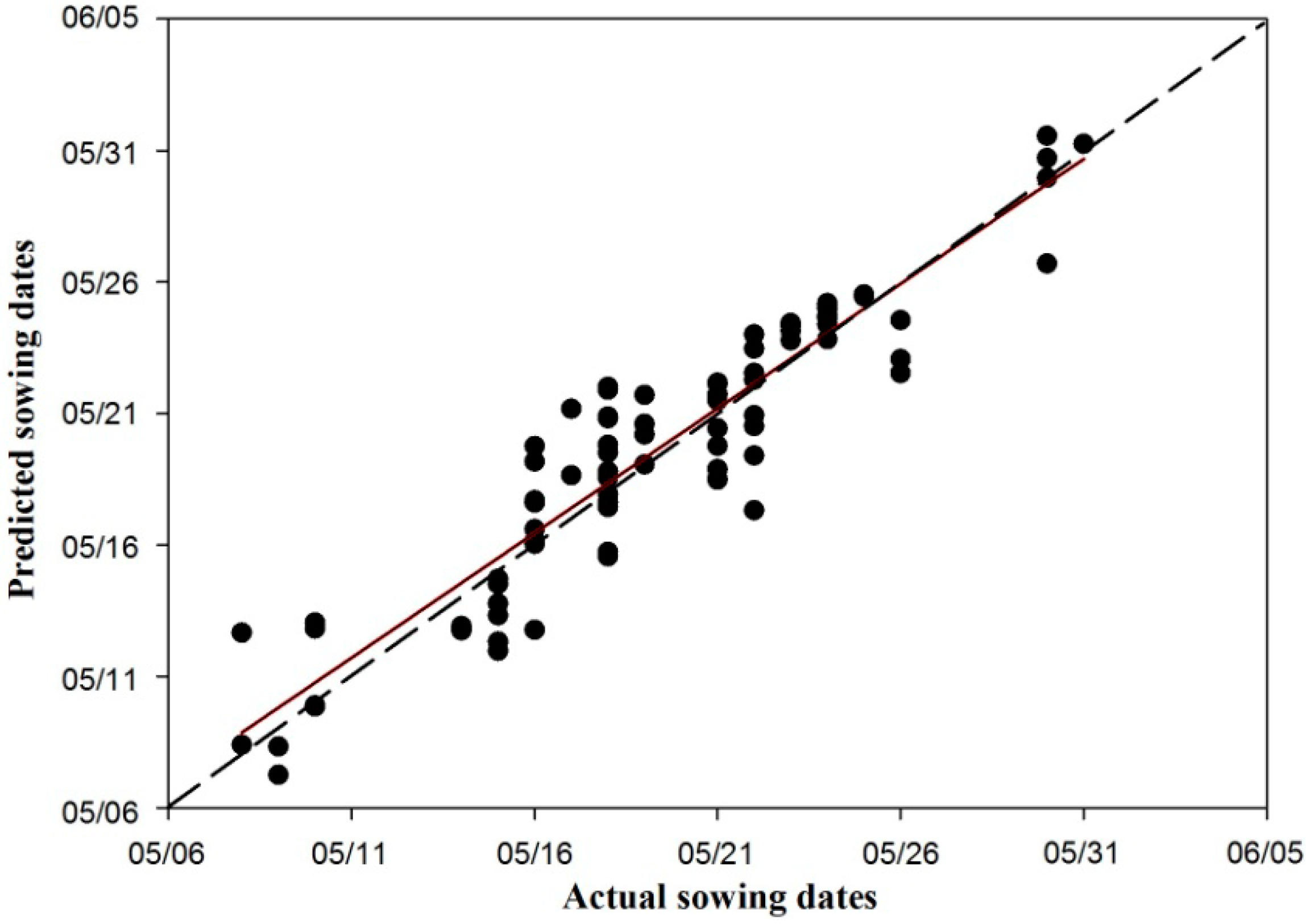
5.2. Sowing Date Monitoring by Polarimetric Parameters in the Early Season
| Acquisition Date | Parameters | 66 Fields for Calibration | 22 Fields for Validation | |
|---|---|---|---|---|
| Linear Model | R² | RMSE (d) | ||
| 16 June | Span | y = 0.0152x − 0.2353 | 0.91 | 2.6 |
| Volume | y = 0.0106x − 0.2004 | 0.94 | 2.4 | |
| Volume/Total | y = 0.0123x + 0.1155 | 0.76 | 5.8 | |
| Odd/Total | y = −0.0109x + 0.8183 | 0.74 | 6.1 | |
| Entropy | y = 0.0083x + 0.4122 | 0.81 | 5.8 | |
| Alpha | y = 0.4311x + 14.652 | 0.78 | 6.8 | |
| 10 July | Span | y = −0.0046x + 0.526 | 0.67 | 6.9 |
| Volume | y = −0.0006x + 0.2688 | 0.04 | - | |
| Volume/Total | y = 0.0103x + 0.29 | 0.81 | 2.8 | |
| Odd/Total | y = −0.0112x + 0.7167 | 0.84 | 2.9 | |
| Entropy | y = 0.005x + 0.6117 | 0.77 | 3.9 | |
| Alpha | y = 0.5499x + 15.143 | 0.84 | 3.3 | |
| 16 June and 10 July | Volume/Total | y = 0.0144x + 0.0658 | 0.95 | 3.1 |
| Odd/Total | y = −0.0149x + 0.9196 | 0.95 | 3.1 | |
| Entropy | y = 0.0087x + 0.4094 | 0.94 | 3.9 | |
| Alpha | y = 0.674x + 8.1788 | 0.95 | 3.2 | |
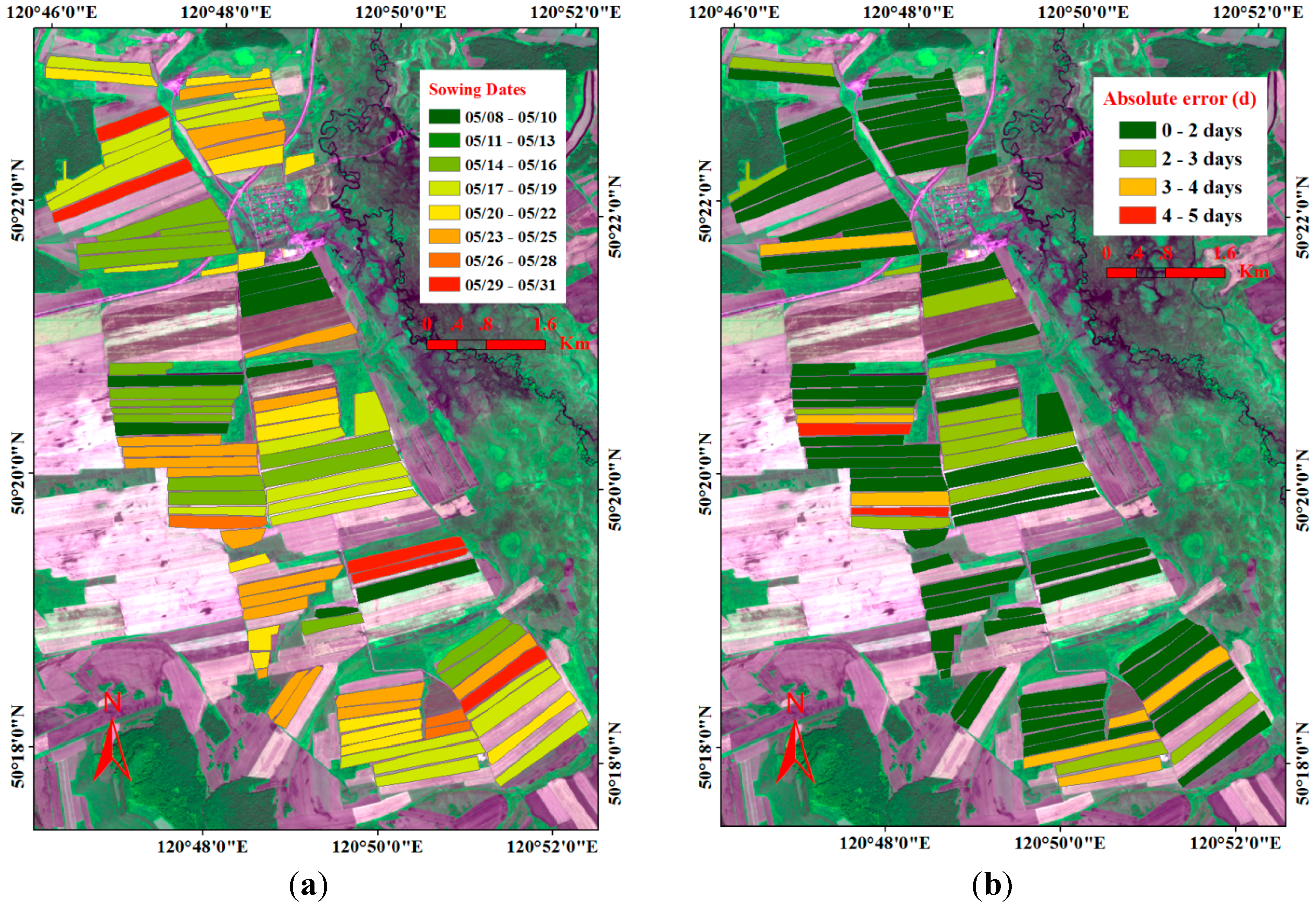
5.3. Mapping Result of Oilseed Rape Fields
5.4. Discussion

6. Conclusions
Acknowledgments
Author Contributions
Conflicts of Interest
References
- Ortiz-Monasterio, J.I.; Dhillon, S.S.; Fischer, R.A. Date of sowing effects on grain-yield and yield components of irrigated spring wheat cultivars and relationships with radiation and temperature in Ludhiana, India. Field Crops Res. 1994, 37, 169–184. [Google Scholar]
- Ortiz-Monasterio, J.I.; Lobell, D.B. Remote sensing assessment of regional yield losses due to sub-optimal planting dates and fallow period weed management. Field Crops Res. 2007, 101, 80–87. [Google Scholar]
- Lobell, D.B.; Ortiz-Monasterio, J.I.; Sibley, A.M.; Sohu, V.S. Satellite detection of earlier wheat sowing in India and implications for yield trends. Agric. Syst. 2013, 115, 137–143. [Google Scholar]
- Muratova, N.; Terekhov, A. Estimation of spring crops sowing calendar dates using MODIS in Northern Kazakhstan. In Proceedings of 2004 IEEE International Geoscience and Remote Sensing SymposiumIGARSS ’04, Anchorage, AK, USA, 20–24 September 2004; Volume 6, pp. 4019–4020.
- Subedi, K.D.; Ma, B.L.; Xue, A.G. Planting date and nitrogen effects on grain yield and protein content of spring wheat. Crop. Sci. 2007, 47, 36–44. [Google Scholar]
- Eslami, H.; Hadi, S.M.; Arabi, M.K. Effect of planting date on protein content of wheat varieties. Int. J. Farming Allied Sci. 2014, 3, 362–364. [Google Scholar]
- Singh, S.; Gupta, A.K.; Gupta, S.K.; Kaur, N. Effect of sowing time on protein quality and starch pasting characteristics in wheat (Triticum aestivum L.) genotypes grown under irrigated and rain-fed conditions. Food Chem. 2010, 122, 559–565. [Google Scholar]
- Leenhardt, D.; Lemaire, P. Estimating the spatial and temporal distribution of sowing dates for regional water management. Agric. Water Manag. 2002, 55, 37–52. [Google Scholar]
- Moulin, S.; Bondeau, A.; Delecolle, R. Combining agricultural crop models and satellite observations: From field to regional scales. Int. J. Remote Sens. 1998, 19, 1021–1036. [Google Scholar]
- Leinenkugel, P.; Kuenzer, C.; Oppelt, N.; Dech, S. Characterisation of land surface phenology and land cover based on moderate resolution satellite data in cloud prone areas—A novel product for the Mekong Basin. Remote Sens. Environ. 2013, 136, 180–198. [Google Scholar]
- Tan, B.; Morisette, J.T.; Wolfe, R.E.; Gao, F.; Ederer, G.A.; Nightingale, J.; Pedelty, J.A. An enhanced TIMESAT algorithm for estimating vegetation phenology metrics from MODIS data. IEEE. J. Sel. Top. Appl. Earth Obs. 2011, 4, 361–371. [Google Scholar]
- Wagenseil, H.; Samimi, C. Assessing spatio-temporal variations in plant phenology using Fourier analysis on NDVI time series: Results from a dry savannah environment in Namibia. Int. J. Remote Sens. 2006, 27, 3455–3471. [Google Scholar]
- Sakamoto, T.; Yokozawa, M.; Toritani, H.; Shibayama, M.; Ishitsuka, N.; Ohno, H. A crop phenology detection method using time-series MODIS data. Remote Sens. Environ. 2005, 96, 366–374. [Google Scholar]
- Wu, W.B.; Yang, P.; Tang, H.J.; Zhou, Q.B.; Chen, Z.X.; Shibasaki, R. Characterizing spatial patterns of phenology in cropland of China based on remotely sensed data. Agric. Sci. China 2010, 9, 101–112. [Google Scholar]
- Mattia, F.; le Toan, T.; Picard, G.; Posa, F.I.; D’Alessio, A.; Notarnicola, C.; Pasquariello, G. Multitemporal C-band radar measurements on wheat fields. IEEE Trans. Geosci. Remote Sens. 2003, 41, 1551–1560. [Google Scholar]
- Liu, C.; Shang, J.; Vachon, P.W.; McNairn, H. Multiyear crop monitoring using polarimetric Radarsat-2 data. IEEE Trans. Geosci. Remote Sens. 2013, 51, 2227–2240. [Google Scholar]
- Shi, L.; Zhang, L.; Yang, J.; Zhang, L.; Li, P. Supervised graph embedding for polarimetric SAR image classification. IEEE Geosci. Remote Sens. Lett. 2013, 10, 216–220. [Google Scholar]
- Lopez-Sanchez, J.M.; Cloude, S.R.; Ballester-Berman, J.D. Rice phenology monitoring by means of SAR polarimetry at X-band. IEEE Trans. Geosci. Remote Sens. 2012, 50, 2695–2709. [Google Scholar]
- Lopez-Sanchez, J.M.; Vicente-Guijalba, F.; Ballester-Berman, J.D.; Cloude, S.R. Polarimetric response of rice fields at C-band: Analysis and phenology retrieval. IEEE Trans. Geosci. Remote Sens. 2014, 52, 2977–2993. [Google Scholar]
- McNairn, H.; Hochheim, K.; Rabe, N. Applying polarimetric radar imagery for mapping the productivity of wheat crops. Can. J. Remote Sens. 2004, 30, 517–524. [Google Scholar]
- Hajnsek, I.; Jagdhuber, T.; Schon, H.; Papathanassiou, K.P. Potential of estimating soil moisture under vegetation cover by means of PolSAR. IEEE Trans. Geosci. Remote Sens. 2009, 47, 442–454. [Google Scholar]
- Cloude, S.R. Polarisation: Applications in Remote Sensing; Oxford University Press: Oxford, UK, 2009. [Google Scholar]
- Adams, J.R.; Rowlandson, T.L.; McKeown, S.J.; Berg, A.A.; McNairn, H.; Sweeney, S.J. Evaluating the Cloude–Pottier and Freeman–Durden scattering decompositions for distinguishing between unharvested and post-harvest agricultural fields. Can. J. Remote Sens. 2013, 39, 318–327. [Google Scholar]
- Cloude, S.R.; Pottier, E. An entropy based classification scheme for land applications of polarimetric SAR. IEEE Trans. Geosci. Remote Sens. 1997, 35, 68–78. [Google Scholar]
- Freeman, A.; Durden, S.L. A three-component scattering model for polarimetric SAR data. IEEE Trans. Geosci. Remote Sens. 1998, 36, 963–973. [Google Scholar]
- Vicente-Guijalba, F.; Martinez-Marin, T.; Lopez-Sanchez, J.M. Crop phenology estimation using a multitemporal model and a Kalman filtering strategy. IEEE Geosci. Remote Sens. Lett. 2014, 11, 1081–1085. [Google Scholar]
- Fieuzal, R.; Baup, F.; Marais-Sicre, C. Monitoring wheat and rapeseed by using synchronous optical and radar satellite data—From temporal signatures to crop parameters estimation. Adv. Remote Sens. 2013, 2, 162–180. [Google Scholar]
- Wiseman, G.; McNairn, H.; Homayouni, S.; Shang, J. RADARSAT-2 Polarimetric SAR response to crop biomass for agricultural production monitoring. IEEE. J. Sel. Top. Appl. Earth Obs. 2014. [Google Scholar] [CrossRef]
- Larranaga, A.; Alvarez-Mozos, J.; Albizua, L.; Peters, J. Backscattering behavior of rain-fed crops along the growing season. IEEE Geosci. Remote Sens. Lett. 2013, 10, 386–390. [Google Scholar]
- Balenzano, A.; Mattia, F.; Satalino, G.; Davidson, M. Dense temporal series of C- and L-band SAR data for soil moisture retrieval over agricultural crops. IEEE. J. Sel. Top. Appl. Earth Obs. 2011, 4, 439–450. [Google Scholar]
- Satalino, G.; Balenzano, A.; Mattia, F.; Davidson, M. C-band SAR data for mapping crops dominated by surface or volume scattering. IEEE Geosci. Remote Sens. Lett. 2013, 11, 384–388. [Google Scholar]
- Meier, U. Growth Stages of Mono-and Dicotyledonous Plants. Available online: http://www.bba.de/veroeff/bbch/bbcheng.pdf (accessed on 17 October 2014).
- Koppe, W.; Gnyp, M.L.; Hütt, C.; Yao, Y.; Miao, Y.; Chen, X.; Bareth, G. Rice monitoring with multi-temporal and dual-polarimetric TerraSAR-X data. Int. J. Appl. Earth Obs. Geoinf. 2013, 21, 568–576. [Google Scholar]
- Lee, J.S.; Pottier, E. Polarimetric Radar Imaging: From Basics to Applications; CRC Press, Taylor & Francis Group: New York, NY, USA, 2009. [Google Scholar]
- Sheng, Y.; Alsdorf, D.E. Automated georeferencing and orthorectification of Amazon basin-wide SAR mosaics using SRTM DEM data. IEEE Trans. Geosci. Remote Sens. 2005, 43, 1929–1940. [Google Scholar]
- Gens, R.; Pottier, E.; Atwood, D.K. Geocoding of polarimetric processing results: Alternative processing strategies. Remote Sens. Lett. 2013, 4, 39–45. [Google Scholar]
- Boerner, W.M.; Mott, H.; Livingstone, C.; Brisco, B.; Brown, R.; Paterson, J.S.; Luneburg, E.; van Zyl, J.J.; Randall, D.; Budkewitsch, P. Polarimetry in remote sensing: Basic and applied concepts. In The Manual of Remote Sensing: Principles and Applications of Imaging Radar, 3rd ed.; Ryerson, R.A., Ed.; American Society for Photogrammetry and Remote Sensing: Bethesda, MD, USA, 1998; pp. 271–357. [Google Scholar]
- Cable, J.; Kovacs, J.; Jiao, X.; Shang, J. Agricultural monitoring in northeastern Ontario, Canada, using multi-temporal polarimetric RADARSAT-2 Data. Remote Sens. 2014, 6, 2343–2371. [Google Scholar]
- Wang, X.; Ge, L.; Li, X. Pasture monitoring using SAR with COSMO-SkyMed, ENVISAT ASAR, and ALOS PALSAR in Otway, Australia. Remote Sens. 2013, 5, 3611–3636. [Google Scholar]
- Ali, I.; Schuster, C.; Zebisch, M.; Forster, M.; Kleinschmit, B.; Notarnicola, C. First results of monitoring nature conservation sites in alpine region by using very high resolution (VHR) X-band SAR data. IEEE. J. Sel. Top. Appl. Earth Obs. 2013, 6, 2265–2274. [Google Scholar]
- McNairn, H.; Wiseman, G.; Powers, J.; Merzouki, A.; Shang, J. Assessment of disease risk in oilseed rape using multi-frequency SAR: Preliminary results. In Proceedings of EUSAR 2014—10th European Conference on Synthetic Aperture Radar, Berlin, Germany, 2–6 June 2014; pp. 747–750.
- Li, K.; Brisco, B.; Yun, S.; Touzi, R. Polarimetric decomposition with RADARSAT-2 for rice mapping and monitoring. Can. J. Remote Sens. 2012, 38, 169–179. [Google Scholar]
- Lopez-Sanchez, J.M.; Ballester-Berman, J.D.; Hajnsek, I. First results of rice monitoring practices in Spain by means of time series of TerraSAR-X dual-pol images. IEEE. J. Sel. Top. Appl. Earth Obs. 2011, 4, 412–422. [Google Scholar]
- Kim, Y.; Lee, H.; Hong, S. Continuous monitoring of rice growth with a stable ground-based scatterometer system. IEEE Geosci. Remote Sens. Lett. 2013, 10, 831–835. [Google Scholar]
- Kim, Y.; Jackson, T.; Bindlish, R.; Hong, S.; Jung, G.; Lee, K. Retrieval of wheat growth parameters with radar vegetation indices. IEEE Geosci. Remote Sens. Lett. 2014, 11, 808–812. [Google Scholar]
- Sakamoto, T.; Wardlow, B.D.; Gitelson, A.A.; Verma, S.B.; Suyker, A.E.; Arkebauer, T.J. A two-step filtering approach for detecting maize and soybean phenology with time-series MODIS data. Remote Sens. Environ. 2010, 114, 2146–2159. [Google Scholar]
- Vyas, S.; Nigam, R.; Patel, N.K.; Panigrahy, S. Extracting regional pattern of wheat sowing dates using multispectral and high temporal observations from Indian geostationary satellite. J. Indian Soc. Remote Sens. 2013, 41, 855–864. [Google Scholar]
- Inoue, Y.; Sakaiya, E.; Wang, C. Capability of C-band backscattering coefficients from high-resolution satellite SAR sensors to assess biophysical variables in paddy rice. Remote Sens. Environ. 2014, 140, 257–266. [Google Scholar]
© 2014 by the authors; licensee MDPI, Basel, Switzerland. This article is an open access article distributed under the terms and conditions of the Creative Commons Attribution license (http://creativecommons.org/licenses/by/4.0/).
Share and Cite
Yang, H.; Li, Z.; Chen, E.; Zhao, C.; Yang, G.; Casa, R.; Pignatti, S.; Feng, Q. Temporal Polarimetric Behavior of Oilseed Rape (Brassica napus L.) at C-Band for Early Season Sowing Date Monitoring. Remote Sens. 2014, 6, 10375-10394. https://doi.org/10.3390/rs61110375
Yang H, Li Z, Chen E, Zhao C, Yang G, Casa R, Pignatti S, Feng Q. Temporal Polarimetric Behavior of Oilseed Rape (Brassica napus L.) at C-Band for Early Season Sowing Date Monitoring. Remote Sensing. 2014; 6(11):10375-10394. https://doi.org/10.3390/rs61110375
Chicago/Turabian StyleYang, Hao, Zengyuan Li, Erxue Chen, Chunjiang Zhao, Guijun Yang, Raffaele Casa, Stefano Pignatti, and Qi Feng. 2014. "Temporal Polarimetric Behavior of Oilseed Rape (Brassica napus L.) at C-Band for Early Season Sowing Date Monitoring" Remote Sensing 6, no. 11: 10375-10394. https://doi.org/10.3390/rs61110375