Article

Estimation of Forest Height Using Spaceborne Repeat-Pass L-Band InSAR Correlation Magnitude over the US State of Maine

Department of Electrical and Computer Engineering, University of Massachusetts Amherst, 151 Holdsworth Way, Amherst, MA 01003, USA
*
Author to whom correspondence should be addressed.
Remote Sens. 2014, 6(11), 10252-10285; https://doi.org/10.3390/rs61110252
Submission received: 27 July 2014 / Revised: 10 October 2014 / Accepted: 11 October 2014 / Published: 24 October 2014

Abstract

:
This paper describes a novel, simple and efficient approach to estimate forest height over a wide region utilizing spaceborne repeat-pass InSAR correlation magnitude data at L-band. We start from a semi-empirical modification of the RVoG model that characterizes repeat-pass InSAR correlation with large temporal baselines (e.g., 46 days for ALOS) by taking account of the temporal change effect of dielectric fluctuation and random motion of scatterers. By assuming (1) the temporal change parameters and forest backscatter profile/extinction coefficient follow some mean behavior across each inteferogram; (2) there is minimal ground scattering contribution for HV-polarization; and (3) the vertical wavenumber is small, a simplified inversion approach is developed to link the observed HV-polarized InSAR correlation magnitude to forest height and validated using ALOS/PALSAR repeat-pass observations against LVIS lidar heights over the Howland Research Forest in central Maine, US (with RMSE < 4 m at a resolution of 32 hectares). The model parameters derived from this supervised regression are used as the basis for propagating the estimates of forest height to available interferometric pairs for the entire state of Maine, thus creating a state-mosaic map of forest height. The present approach described here serves as an alternative and complementary tool for other PolInSAR inversion techniques when full-polarization data may not be available. This work is also meant to be an observational prototype for NASA’s DESDynI-R (now called NISAR) and JAXA’s ALOS-2 satellite missions.

Graphical Abstract

1. Introduction

A spaceborne satellite mission with radar and lidar would have the capability of mapping the global vegetation structural information at fine resolutions, which is important to understand and monitor the global carbon budget and climate change. To address this need, NASA envisioned the DESDynI mission (originally to include both radar and lidar) as a high priority in the current decade. In 2011, the lidar portion of DESDynI was effectively cancelled [1], thus placing an increased emphasis on the remaining radar portion (called DESDynI-R or NISAR). In accordance with this change, algorithms associated with radar’s capabilities for resolving vegetation biophysical information will need to be configured in such a way as to make due with the satellite’s new configuration.
Multi-baseline, single-pass InSAR/PolInSAR correlation observations have been shown to be sensitive to vegetation vertical structure and forest height through the use of a physical scattering model [2,3], often termed as the Random Volume over Ground (RVoG) model that relates complex correlations to the vegetation structure and/or height. In repeat-pass SAR interferometry however, the additional error source of temporal decorrelation has been observed to affect the correlation measurements to varying degrees [4,5]. The degree of temporal decorrelation is primarily dependent on the changes of the environmental conditions (e.g., moisture [6,7], wind [8,9], tree regrowth [10], freezing [11]) during the repeat period (referred to as “temporal baseline”), with the thought that the longer temporal baseline, the more likely the environmental conditions will change a lot. In this paper, we will use the term “temporal baseline” to characterize the possibility of weather changes.
Generally speaking, in repeat-pass InSAR applications, the RVoG model has also been successfully used to provide estimates of forest heights with airborne temporal baselines of 40 minutes at both L- and P-band [12]. For moderate temporal baselines (i.e., less than 15 days), modified versions of the RVoG model have been demonstrated to account for the effect of ground dielectric change and random motion of the volume scatterers [6,13]. To this end, Askne et al. [8] and Lavalle et al. [9,14] introduce a coordinate-dependent vertical motion profile which can be incorporated into the RVoG model characterizing the wind-induced temporal decorrelation.
For spaceborne repeat-pass InSAR systems with large temporal baselines (on the order of months; at least 46 days for ALOS), the effect of temporal decorrelation (e.g., both dielectric change and random motion) often dominates the correlation observations even under the condition of small kz (vertical wavenumber) so that the observed correlation magnitudes are relatively low. Without a proper modification of the RVoG model, the interpretation and utility of the spaceborne repeat-pass InSAR correlation data is constrained.
In the work presented here, a semi-empirical version of the repeat-pass InSAR correlation model is used to estimate forest height in the US state of Maine. This is achieved by augmenting the random motion model developed in [8,9] so that the repeat-pass InSAR correlation model includes the effect from dielectric change in the target, which has the effect of changing the correlation by a height-independent constant. By assuming (1) the temporal change parameters and forest backscatter profile/extinction coefficient follow some mean behavior across each inteferogram; (2) the ground scattering contribution is minimal for cross-polarization; and (3) the vertical wavenumber is small, a simplified inversion approach is developed to link the observed HV-polarized InSAR correlation magnitude to forest height with the model parameters characterizing the temporal change effects (both dielectric change and random motion). These model parameters are thus determined by fitting the ALOS InSAR-inverted forest height with full-waveform lidar data collected over a 63 km by 7 km region (44,000 hectares) in central Maine, US covered by the LVIS sensor. The temporal change parameters derived from this supervised regression are used as the basis for propagating the height estimates to available interferometric pairs for the entire state of Maine, thus creating a state-mosaic map of forest height.
This paper begins by demonstrating the modified repeat-pass InSAR correlation model (Section 2), followed by the simplified forest height inversion approach along with the simulation results (Section 3). Section 4 describes the study area as well as the experimental data utilized in Section 5, where validation results and discussions will be shown. This paper concludes with Section 6 and three appendices which discuss the fundamental assumptions utilized in this paper.

2. Theory

For moderate temporal baselines (i.e., less than 15 days), modified versions of the RVoG model have been demonstrated to account for the effect of dielectric change and random motion of the scatterers [6,13,15] by incorporating a multiplicative temporal correlation factor. Askne et al. [8] and Lavalle et al. [9,14] introduce a vertical motion profile which is incorporated into the RVoG model in order to characterize a wind-induced temporal decorrelation. The results from these papers [8,9] are augmented so that the modified RVoG model presented here can be formulated as below for spaceborne repeat-pass InSAR systems with large temporal baselines (on the order of months; at least 46 days for ALOS), where temporal decorrelation from both dielectric change and random motion will dominate. Particularly, the correlation component of the coupled effect from volume scattering and temporal change is written as
γ v & t   =     γ d v γ v & m   + γ d g m 1 + m
with
γ v & m = exp [ 1 2 ( 4 π λ ) 2 σ r 2 ( z ) ] σ V ( z ) exp ( j k z z ) d z σ V ( z ) d z
where m is the ground-to-volume ratio, and σV(z) is the extinction-weighted backscattering profile for the volume only. The variables γdv and γdg represent the temporal correlation component due to dielectric change for the volume and the underlying ground, respectively, and γv&m is the coupled correlation component due to volume scattering and random motion. In the above, kz is the vertical wavenumber (in units of rad/m), σr(z) is the random motion standard deviation along the line of sight, and λ is the wavelength.
The motion standard deviation in Equation (2) is here assumed to be linear as a function of height, i.e.,
σ r ( z ) = σ r h r z
where σr denotes the motion standard deviation at some reference height hr(selected to be 15 m in this work and also as in [9]). Equation (3) is equivalent to [8] and in contrast to [9] (where the motion variance is assumed linear in the vertical coordinate) because results created using the assumption in Equation (3) created a “best fit” between ground validation observations and height in this application (to be discussed later in Section 5.2). Moreover, the ground motion term used in [9] is not used in this model since the wind-induced ground-motion is expected to be small in comparison to volume-motion. In contrast, dielectric change of the ground surface is accounted for by including a term for ground dielectric change, γgd, as in [6,8,13].
The model parameters, γdv, γdg and σr, in Equation (1) through Equation (3) are a function of the d temporal decorrelation, which is target dependent [4,5] and results from a combination of factors, including wind and rain effects [6,8,9,13]. Even though these factors are expected to be spatially varying throughout a scene, it is reasonable to assume that they follow some degree of mean behavior (Appendix A), and it is this behavior that the model is meant to use for estimating forest height. For those interferograms where the spatial variation is non-stationary, or that the spatial variation is the dominant signature, the interferogram may be eliminated and another used in its place given plenty of interferograms over the same area (e.g., it is not uncommon that dozens of interferograms from ALOS/PALSAR are available). This is possible, because the errors that appear due to spatially varying temporal decorrelation, are detectable within individual scenes (showing up as non-physical height estimates), and when scenes are mosaicked together, because of large differences in forest height solutions between adjacent scenes.
By setting γdv = Sscene and γdg = S′scene, and substituting Equation (3) into Equation (1), a general model for the combined volumetric and temporal decorrelation can be written as
γ v & t = S s c e n e γ v & m + µ m 1 + m
With
γ v & m = exp [ 1 2 ( 4 π σ r λ h r ) 2 z 2 ] σ V ( z ) exp ( j k z z ) d z σ V ( z ) d z
and
µ = S s c e n e S s c e n e
where Sscene and S′scene are complex numbers with magnitudes less than or equal to one, and µ being the “ground-to-volume ratio” of the temporal decorrelation induced by dielectric fluctuations, which has a complex value with |µ| ∈ [0, ∞).
The values of Sscene, S′scene and m are polarization-dependent, making the use of Equation (4) through Equation (6) potentially very difficult. Simplified scenarios where this polarization dependence is reduced (e.g., [13,15]) are often used under the assumption of short temporal baselines [6,13], in order to apply PolInSAR techniques [3]. When the time between observations for an interferometric pair is on the order of months, both Sscene and S′scene are expected to be strongly polarization-dependent, which makes the PolInSAR formulation of determining the vegetation height an underdetermined problem. In this study, we investigate the effect of this polarization-dependence on the inversion using HH-pol and HV-pol channels (Appendix B), although ultimately, it is the HV-pol data that is used for forest height inversion.

3. Forest Height Inversion Approach

In this section, a simplified semi-empirical forest height inversion method is first introduced and then implemented through the use of a Least Squares curve fitting. Simulated inversion results based on this are demonstrated as well. As an overall guide, the flowchart is demonstrated below in Figure 1 showing the associated InSAR processing and inversion procedure. Specifically, Section 3.1 derives the simplified inversion model, Section 3.2 describes the nonlinear Least Squares fitting with the Gauss-Newton numerical method, and the InSAR processing details will be provided in Section 5.1.
Figure 1. Flowchart of the InSAR processing and the inversion procedure. The sinc inversion model and the Gauss-Newton algorithm are discussed in Section 3.1 and Section 3.2, respectively, while InSAR processing details are to be provided in Section 5.1.
Remotesensing 06 10252 g001

3.1. Simplified Model of |γv&t|

In practice, there is always a ground scattering component (i.e., m 0 in Equation (1)) over bare surfaces or sparse forests. It is also possible that a polarization-dependence exists for the parameters m and µ (see previous section). In Appendix B, simulation results are demonstrated on the performance of the forest height inversion model presented here for HH-pol (characterized by a large value for m) and HV-pol (characterized by a small value for m) data with various choices of µ. Because of the second-order scattering dependence of cross-polarized fields, it is observed that for HV-pol data, the assumption of a small m (not necessarily to be zero) with µ close to 1 works well over almost the entire height range and hence performance of this inversion approach is equivalent to the case of m = 0. Therefore, the absence of a ground-scattering term (i.e., m = 0 [9,12]; see also Appendix B), for cross-polarized fields is assumed here only in order to simplify the analysis and the derivation of the semi-empirical forest height inversion model.
By making this assumption, Equation (4) is reduced to
γ v & t = S s c e n e exp [ 1 2 ( 4 π σ r λ h r ) 2 z 2 ] σ V ( z ) exp ( j k z z ) d z σ V ( z ) d z
This expression is further simplified under the zero-baseline scenario (only to simplify the derivation; to be discussed later), when kz = 0, where Equation (7) is rewritten as
γ v & t = S s c e n e exp [ 1 2 ( 4 π σ r λ h r ) 2 z 2 ] σ V ( z ) d z σ V ( z ) d z
By utilizing the mean value theorem for integration, it can be shown that there exists an intermediate height, ξ, between the ground and the maximum forest height, hv, (i.e., ξ [0, hv]) such that Equation (8) can be rewritten as
γ v & t = S s c e n e exp [ 1 2 ( 4 π σ r λ h r ) 2 ξ 2 ]
Assuming forests with different height values are of the scaled versions of extinction-weighted backscattering profile and height-dependent motion profile (in Section 3.3 both extinction coefficient and random motion level are considered constant in the mean’s sense in order to ensure this assumption; see Appendix A), ξ is thus proportional to hv, i.e., ξ = αhv with the proportionality constant 0 α 1. Therefore, we have
| γ v & t | = S s c e n e exp [ 1 2 ( 4 π σ r α λ h r ) 2 h v 2 ] S s c e n e sinc ( h v C s c e n e ) ,  for  h v < π C s c e n e
where
C s c e n e = λ h r   2 π 2 σ r   α
After taking the magnitude of γv&t, Sscene becomes |Sscene|; however, in order to maintain a concise notation, Sscene is used here instead of |Sscene|, with the exact definition of Sscene allowed to be inferred from the context. Here, the scaling factor Cscene primarily relates to the random motion level (e.g., due to wind and/or tree regrowth) of the volume scatterers. At the current stage, we know that the higher dielectric change is, the smaller Sscene we have, while the greater random motion is, the smaller Cscene we have.
Note, importantly, that the sinc function in Equation (10) is used to approximate the “Gaussian-like” function in the derivation. This has the benefit of obtaining an upper limit (i.e., πCscene) on the maximum inverted height in the presence of uncertainty in measuring the correlation. Without this simplifying approximation, the expression in Equation (10) is significantly more complicated and the inverted height will approach infinity as the observed correlation magnitude becomes very low. This is also important, because there is a large uncertainty in estimating low correlation magnitude signals (<0.2; [16]) when the number of sampled looks is small, as is usually the case for spaceborne missions (e.g., 20 looks were used in the study presented here). In such a scenario, the estimation error encountered in the inversion of the Gaussian function of Equation (10) will create significant errors in the long “tail” regions of a Gaussian curve, as the forest heights get larger.
Futhermore, for spaceborne repeat-pass InSAR systems, it is difficult to have kz = 0, and therefore it is also not possible to separate its effect from Equation (7). Small values of kz (<0.15 rad/m; which is taken as the effective range of kz values for this study in Appendix C) can be accommodated by the model in Equation (10) under a small-kz assumption (described in Appendix C). This assumption manifests itself as a bias in Equation (8) and a kz-dependent correction factor is included in α (and thus Cscene) in Equation (11). Hence, under the small-kz assumption, α depends on the extinction-weighted backscattering profile, the height-dependent motion profile, and kz. If a uniform backscattering profile along with an exponential extinction profile is considered (as used in Section 3.3), α (and thus Cscene) only depends on the extinction coefficient (denoted by ke), random motion level σr and vertical wavenumber kz, and can be written as
α = α (ke, σr, kz)
It should be noted that the sinc function of Equation (10) is not related to the sinc solution derived for forest height estimation in Polarization Coherence Tomography, PCT [17], where a uniform extinction-weighted backscattering profile is assumed in the absence of temporal change effects. In deriving Equation (10), a small-kz assumption (see Appendix C) is used, and thus the temporal decorrelation effects from dielectric fluctuations and random motion dominate the repeat-pass InSAR correlation rather than the volumetric component associated with PCT. In Equation (10), Sscene derives from the target dielectric change (perhaps due to moisture change, e.g., rain), while Cscene (defined as Equation (11)) primarily describes the level of random motion (resulting from wind and/or changes in the forest structure). While the expression in Equation (10) is not restricted to uniform profiles, in the simulations that follow (Section 3.3), a uniform backscattering profile with an exponential extinction profile are used in order to illustrate how the model behaves under conditions of varying motion and forest height.
Since this model utilizes the temporal change effects (both dielectric change and random motion) under the conditions of small, but not zero, values of kz, the performance of this inversion approach does not rely on the ground topography.

3.2. Forest Height Inversion by Estimating the Fitting Parameters Sscene and Cscene

Before we look at the parameter estimation, we first discuss and define the resolution in this work. As will be shown later in Section 5.1, all of the interferograms in this paper are at a resolution of 20 m × 30 m. However, due to the observational error in the correlation measurements (i.e., correlation sampling noise [16]) and the target-dependent behavior of the temporal change effects (which is different from stand to stand), spatial averaging (which is referred to as “multi-pixel averaging” in this work) must be performed in order to remove these uncertainties. This gives resolution on the order of 20–30 hectares with RMSE < 4 m.
The observed repeat-pass InSAR correlation magnitude, |γv&t|, due to the coupled effect of volume scattering and temporal change can be related to the desired height estimates, hv, by analytically inverting Equation (10) over the region of validity, hv < πCscene. An equivalent, more computationally efficient approach, is to use a look-up table. In either case, forest height estimates are based on the fitting parameters, Sscene and Cscene. These parameters can be determined from overlap with regions of known forest height (such as where lidar data is available), or in overlap regions of scenes created by adjacent orbits or along-track observations of the satellite. The process of estimating values of Sscene and Cscene follows.
In these overlap areas, the set of known heights can be written as, hv1, which are considered as the reference. The heights determined by Equation (10) are specified as hv2, and are dependent on both the observed correlation magnitude and the model parameters, Sscene and Cscene. With a set of initial values for Sscene and Cscene, a scatter plot of hv1 versus hv2 can be made, such as that shown in Figure 2, where the cloud of data points, on a pixel-by-pixel basis are illustrated by an ellipse.
Figure 2. Geometric illustration of the comparison between two sets of height estimates. The data cloud is considered an ellipse, with the angle between the major axis and the horizontal axis denoted by φ, and their average heights denoted as m1 and m2. Here Height 1 is considered as the reference height.
Remotesensing 06 10252 g002
Ideally, all points in these overlap regions would follow along the diagonal representing the 1:1 line in Figure 2, and in the presence of error sources, would have the ellipse align itself along the line. In general, this is not the case, and there is a offset associated with the location of the ellipse centroid, and its tilt angle. Both of these parameters can be determined through an optimization procedure which will achieve this alignment.
To achieve this goal, a principal components analysis routine [18] was used here to determine the slope k of the ellipse’s major axis (i.e., the tangent of the tilt angle ϕ shown in Figure 2), and the offset b of the ellipse centroid from the 1:1 line (i.e., the relative difference between the mean heights m1 and m2 in Figure 2). Therefore, we have the following definitions for k and b, i.e.,
k = tan ϕ b =     m 1 m 2   ( m 1 + m 2 ) / 2  
Specifically, in order to solve for the slope k, we denote hv1(i) and hv2(i) to be the reference height and the InSAR-inverted height for the ith averaged pixel. Suppose there are N averaged pixels in total, we can write the covariance matrix of these two estimates of height as
X _ _   = [ i = 1 N ( h v 1 ( i ) m 1 ) 2 i = 1 N ( h v 1 ( i ) m 1 ) ( h v 2 ( i ) m 2 ) i = 1 N ( h v 1 ( i ) m 1 ) ( h v 2 ( i ) m 2 ) i = 1 N ( h v 2 ( i ) m 2 ) 2 ] = [ P 11 P 12 P 21 P 22 ] [ λ 1 0 0 λ 2 ] [ P 11 P 12 P 21 P 22 ] 1
where the eigen value decomposition is applied in the last equation. Here, λ1 and λ2 are the eigen values in the descending order, while [ P 11 P 21 ] and [ P 12 P 22 ] are their corresponding eigen vectors, respectively. Then, the slope k can be calculated as
k = P 21 P 11
With k and b determined, Sscene and Cscene are adjusted such that the long-axis of the ellipse is aligned with the 1:1 line (i.e., k ≈ 1 and b ≈ 0). Hence, we come up with the following fitting metric (denoted as the “k-b” fitting metric), i.e.,
  ( S   s c e n e , C   s c e n e * = a r g m i n S s c e n e , C s c e n e ( k 1 ) 2 + ( b 0 ) 2
which is equivalent to a nonlinear least squares fit (since the fitting parameters k and b are nonlinear functions of the model parameters Sscene and Cscene), where S s c e n e and C s c e n e are the desired optimum values of the model parameters. To solve the above nonlinear least squares problem, a Gauss-Newton algorithm [19] is applied, i.e.,
[ S   s c e n e * C s c e n e   ] = ( J _ _ T   J _ _ ) 1 J _ _ T [ 1 k 0 0 b 0 ] + [ S s c e n e 0 C s c e n e 0 ]
where Sscene0 and Cscene0 are the initial guess of the model parameters, and k0 and b0 are the fitting parameters corresponding to this initial case. The matrix J _ _ is the Jacobian matrix (calculated at the initial point) that is defined as in Equation (18) and can be computed numerically, i.e.,
J _ _ = [ k S s c e n e k C s c e n e b S s c e n e b C s c e n e ] | S s c e n e 0 C s c e n e 0
The Gauss-Newton algorithm is an iterative numerical method, which iteratively considers the derived model parameters on the left-hand side of Equation (17) as the new initial point for another circulation of Equation (17). Regardless of the accuracy of the initial point, convergence for the type of data in the present work has been achieved after the third iteration.
An alternative to the “k-b” fitting metric would be to use the Euclidean norm instead. This is successful when the Root Mean Squared Error (RMSE) between the ground validation and initial height estimates is small. However, when the RMSE is large, i.e., >3 m, the “k-b” fitting metric proves more robust. An example is shown in Figure 3, where the input data RMSE is 3.9 m. This figure shows the residual error plotted as a function of Sscene and Cscene, the two parameters that are being determined, using the two different error metrics: the Euclidian norm (Figure 3a) and the “k-b” fitting metric (Figure 3b). As can be seen in the set of figures, it is difficult to determine the global minimum using the Euclidean norm, whereas the “k-b” fit is much more well behaved. The reason is that when the RMSE is large, the Euclidean norm metric is not sensitive to the orientation of the data cloud depicted in Figure 2. Here, even though the RMSE will be small, it will not guarantee a good linear relationship with the ground validation data. Use of the “k-b” metric, as described in Equation (16), and illustrated in Figure 3b, the global minimum is better defined and guarantees this linear relationship (since k ≈ 1) while also maintaining a small RMSE.
Figure 3. The two dimensional residual error distribution over the Sscene and Cscene plane with (a) the Euclidean norm as the fitting metric and (b) the “k-b” fitting metric for the experimental data with RMSE of 3.9 m.
Remotesensing 06 10252 g003

3.3. Simulation Results

The correlation due to the coupled effect of volume scattering and temporal change can be simulated by numerically computing the integral in Equation (7), while the height estimates obtained from the simulations are determined by inverting Equation (10) through the adjustment of the model parameters Sscene and Cscene (Section 3.2). For the extinction-weighted backscattering profile in Equation (7), σV(z), a uniform backscattering profile along with an exponential extinction profile are used. The basic simulation parameters are chosen such that the extinction coefficient ke = 0.1 dB/m (e.g., a sparse forest; less than the values used in [3,9] at L-band), the vertical wavenumber kz = 0.05 rad/m (corresponding to B = 500 m with ALOS’s viewing geometry), the magnitude of the correlation component due to dielectric fluctuation Sscene = 0.7 and the motion standard deviation σr = 2 cm at the reference height hr = 15 m (i.e., σr(z) = 0.0013z). By assuming a constant temporal change and forest backscatter profile/extinction coefficient (Appendix A), all of the above parameters are assumed constant in the mean’s sense for different values of forest height. The simulation result is illustrated in Figure 4a, with the left-hand side plot showing the estimated heights compared to the actual height, and the right-hand side showing the simulated correlation magnitude by using Equation (7) compared to the fitted solution of Equation (10). Through curve fitting, the parameter Cscene is determined to be 10.92, which primarily corresponds to σr= 2 cm (at a reference height of hr = 15 m), and Sscene fitted to be 0.7. Using Equation (11), α is calculated to be 0.82. We make a note here that such simulation parameters are selected to mimic the ground validation results of Section 5.
Figure 4. Simulation Results. (a) serves as the basis of the simulations, showing the estimated height vs. the actual height (on the left), and the simulated correlation component vs. the sinc approximation (on the right). The simulation parameters for this basic case are: extinction coefficient of 0.1 dB/m, kz of 0.05 rad/m, Sscene of 0.7, motion standard deviation of 2 cm at the reference height of 15 m. (b) shows the result with a different extinction coefficient (0.3 dB/m); (c) shows the result with a different kz(0 rad/m); while (d) shows the result with a different motion standard deviation (6 cm at the height of 15 m).
Remotesensing 06 10252 g004
In the remaining three simulations of Figure 4, we allow the relevant parameters to vary and study the sensitivity of the inversion results. Specifically, the extinction coefficient is changed to 0.3 dB/m (e.g., a dense forest [9]; Figure 4b), the vertical wavenumber is changed to 0 (zero-baseline; Figure 4c), and the motion standard deviation is changed to 6 cm at hr = 15 m (greater level of random motion; Figure 4d).
It is clear that σr is the most important parameter that dominates the value of Cscene, which is noticed to have a weak dependence on the extinction coefficient. Here, the kz-dependence of Cscene can be ignored for kz’s up to 0.05 rad/m, and plays a weak role for kz < 0.15 rad/m (small kz assumption; Appendix C). Using Equation (11), the α values for all of the three subplots are 0.93, 0.82 and 0.65, respectively, which demonstrates the dependence of α on σr and ke. The kz-dependence of α can be neglected for kz < 0.05 rad/m, although it is noticeable for kz up to 0.15 rad/m (Appendix C).
Larger random motion levels (possibly induced by higher wind speed) results in smaller values of Cscene, which will make the saturation point occur at a low height value. In such a scenario, meaningful forest height inversion will be hindered due to the loss of sensitivity of the model in Equation (10) to changes in forest heights. Similarly, larger dielectric changes (possibly due to moisture change) results in smaller values of Sscene, which will suppress the measured correlation component γv&t (see Equation (7)) by a large amount causing the information to be dominated by the correlation sampling noise [16] as discussed above.

4. Study Area and Experimental Data

In this section, we will first describe the study site in central Maine, US and then introduce the experimental data from LVIS and ALOS/PALSAR.

4.1. Site Description

To validate the inversion model, the chosen study area extends over a 83 km × 71 km region in central Maine (see Figure 5), where the Howland Research Forest (Latitude 45°12’, Longitude −68°43’) and the Penobscot Experimental Forest (Latitude 44°51’, Longitude −68°37’) are located. Two climate observing stations that are close to the Howland forest and the Penobscot forest are illustrated in Figure 5 with the historical weather record available from NOAA’s National Climate Data Center (NCDC) [20].
About 35 miles north of Bangor, ME, the 202-ha Howland research forest is a boreal-northern hardwood transition forest consisting of spruce-hemlock-fir, aspen-birch, and hemlock-hardwood mixtures with average tree height of 20 m [21]. The forest has not been selectively logged since 1900 and is considered as an “overmature” forest. The climate over this area is primarily cold, humid, and continental with the snowpack being of up to 2 m from December through March. The annual temperature and rainfall in this region are measured as 6.1 ± 1.0 °C and 988 ± 170 mm. The topography around this area varies from flat to gently rolling with a maximum elevation change of < 68 m within 10 km.
Similarly, the 1619-ha Penobscot experimental forest adjacent to Bangor, ME across the Penobscot river is located in Acadian Forest, which is an ecotone between the eastern broadleaf and boreal forests consisting of a mixture of northern conifers and hardwoods dominated by spruces, balsam fir, and eastern hemlock [22]. The average tree height is 18.4 m. The climate is cool and humid with the annual temperature average of 6.6 °C (e.g., −7.0 °C for February and 20.0 °C for July). Annual precipitation is about 1060 mm, with 48% falling from May through October, and annual snowfall averages 239 cm.
Figure 5. Study area in Maine, US. The grey image shows the correlation magnitude of the interferogram 10 July–25 August 2007 over the central Maine area, where the Howland research forest and the Penobscot experimental forest are encompassed and marked. The overlaid color map is an LVIS strip of height, and serves as the ground validation data for forest height inversion. Two climate observing stations (“North Station” and “South Station”) are also indicated.
Remotesensing 06 10252 g005

4.2. LVIS Lidar Data

Ground validation data exists in the form of a narrow strip (63 km × 7 km) of Laser Vegetation Imaging Sensor (LVIS; [23]) data collected over the Howland forest and the Penobscot forest in 2009. LVIS is an airborne full-waveform scanning laser altimeter, which is developed by NASA’s Goddard Space Flight Center (GSFC). It operates at an altitude of 10 km producing swath up to 1000 km wide and normally with 25-m wide footprints and 10-cm height accuracy. The LVIS height data in this study is demonstrated as a color strip map in Figure 5 with a spatial resolution of 50 m × 50 m in raster grid.
The data products of LVIS Lidar data has various metrics: RH50, RH75 and RH100, etc. Here, “RH” means relative height, and RH100 height stands for the height above the detected ground at which 100% of the waveform energy has been returned, and is typically associated with the maximum tree height within a resolution beam of the lidar. In this study, RH100 metric is used and found to be well related to the ALOS InSAR-inverted forest heights, as will be shown in Section 5.2.

4.3. ALOS/PALSAR Data

ALOS/PALSAR is a repeat-pass L-band SAR developed by the Japanese Aerospace Explore Agency (JAXA) through the Kyoto and Carbon Initiative (K&C) [24,25]. The repeat period of ALOS/PALSAR is 46 days. In this central Maine area, there also exists eight FBS (fine-beam single-polarization) and ten FBD (fine-beam dual-polarization) ALOS/PALSAR scenes (Table 1). In Table 1, we also show the temperature and the precipitation on the observation date, as well as the accumulated precipitation during the past three days prior to the data collection (denoted as “3-day accumulated precipitation”), all of which are available from NOAA’s NCDC [20]. For each observation date, the weather record for both climate observing stations are demonstrated. The “3-day accumulated precipitation” is used because it happens that there might not be rainfall on the observation date; however, the humidity level is still high due to the accumulated rainfall in the past few days, e.g., “20101018”. It can also be seen that some of the PALSAR scenes have uniform weather conditions over the northern and southern sites, e.g., “20070710”, “20071010” and “20100718”. However, some of them seem to have nonuniform weather conditions (e.g., “20070825”), which we would like to avoid in order to apply the assumption of constant temporal change parameters as discussed above and in Appendix A (i.e., the weather conditions for each acquisition of the interferogram is uniform). Such an effect can be seen in Figure 5 where the grey-scale image shows the correlation magnitude of the interferogram 07/10/2007–08/25/2007. Here, the correlation magnitude is significantly affected by the nonuniform weather conditions on 08/25/2007 due to the rainfall occurred over the northern site.

5. Results and Discussions

In this section, we first validate the presented inversion model by comparing ALOS InSAR correlation magnitude-inverted heights with LVIS heights (i.e., supervised regression) over the Howland and Penobscot forests, then utilize the derived model parameters from central Maine as the basis to create the state mosaic of forest height.

5.1. InSAR Processing

All interferograms described in this paper were created using Gamma Remote Sensing software [26] with a correlation estimation window size of 5 × 5 and a multi-look averaging (two range looks along with ten azimuth looks) afterwards. The data were transformed into map coordinates (at a resolution of 20 m × 30 m) that are coincident with the Shuttle Radar Topography Mission (SRTM) data through a look-up table. The common-band filtering (both range and azimuth) is applied to ensure the geometric decorrelation is removed [27,28]. The estimation bias in the sampled correlation magnitudes and the thermal noise decorrelation are corrected as in [16,29], respectively. The remaining correlation component only deals with the coupled effect of volume scattering and temporal change.
Table 1. ALOS/PALSAR acquisitions over the central Maine area between 2007 and 2011. For each acquisition, weather conditions are provided over the “North Station” (denoted by “(N)”) as well as the “South Station” (denoted by “(S)”). “3-day Accumulated Precipitation” stands for the accumulated precipitation during the past three days prior to the observation date.
Collection DateData ModePrecipitation (mm)3-Day Accumulated Precipitation (mm)Temperature (Max/Min; °C)
20070107FBS7.6 (N)20.6 (N)12.8/3.3 (N)
0.0 (S)16.3 (S)6.7/−3.9 (S)
20070222FBS0.0 (N)1.3 (N)0.0/−15.6 (N)
0.0 (S)0.0 (S)−1.7/−20.6 (S)
20070710FBD2.8 (N)3.3 (N)19.4/9.4 (N)
0.0 (S)0.0 (S)28.9/12.2 (S)
20070825FBD19.1 (N)5.3 (N)22.2/17.8 (N)
1.0 (S)8.4 (S)29.4/15 (S)
20071010FBD0.5 (N)4.6 (N)16.7/3.3 (N)
0.0 (S)1.0 (S)12.2/7.2 (S)
20080110FBS2.5 (N)0.3 (N)11.1/2.8 (N)
0.0 (S)0.3 (S)6.7/−4.4 (S)
20080225FBS0.0 (N)3.8 (N)3.9/−12.2 (N)
0.0 (S)4.3 (S)5/−13.3 (S)
20080411FBS0.0 (N)0.0 (N)12.2/1.1 (N)
0.0 (S)0.0 (S)11.1/0.6 (S)
20080527FBD0.5 (N)2.3 (N)22.2/11.1 (N)
0.0 (S)0.0 (S)26.7/6.7 (S)
20080712FBD0.0 (N)8.6 (N)24.4/8.9 (N)
0.0 (S)0.0 (S)26.1/8.3 (S)
20090227FBS0.3 (N)0.3 (N)2.2/−12.2 (N)
7.6 (S)0.0 (S)8.9/−6.7 (S)
20090830FBD14.0 (N)2.5 (N)11.7/10 (N)
0.0 (S)51.3 (S)21.1/10.6 (S)
20091015FBD0.0 (N)9.1 (N)7.8/−3.3 (N)
0.0 (S)10.2 (S)5.6/−3.9 (S)
20100417FBS0.0 (N)0.0 (N)11.1/0.6 (N)
0.0 (S)0.0 (S)6.1/2.2 (S)
20100602FBD17.8 (N)0.0 (N)15.6/12.2 (N)
0.0 (S)11.4 (S)22.2/12.2 (S)
20100718FBD2.5 (N)0.0 (N)30.6/16.7 (N)
0.0 (S)0.0 (S)28.9/17.2 (S)
20101018FBD0.0 (N)45.2 (N)16.1/4.4 (N)
0.0 (S)41.1 (S)10/1.1 (S)
20110305FBS0.3 (N)1.0 (N)−1.7/−25 (N)
0.5 (S)1.8 (S)5.6/−3.3 (S)
Specifically, common-band filtering was applied to the eight FBS and ten FBD observations so that interferograms could be formed out of all combinations [26]. These were processed into 153 interferograms with the scene-wide correlation magnitude averages and their kz values shown as blue circles in Figure 6. From Figure 6, it can be seen that even for kz < 0.06 rad/m, the ALOS scenes collected between July and October in both 2007 and 2010 have the best correlations amongst the possible combinations (even after accounting for the effects of baseline and volumetric decorrelation). While this may be a surprising result because it implies that the summer/fall data has the best correlations as opposed to winter scenes, we allowed the data to indicate the best scenes to use for this analysis. Such information may be pertinent to future spaceborne missions such as DESDynI-R and ALOS-2. Note that we define the “best” scene as the one with the highest correlation magnitude. Although we utilize the temporal change effects to invert forest height, this does not contradicts considering the “best” scene with highest correlation magnitude (or equivalently the least temporal change effects). As seen in Figure 6, even for the best interferometric pair 07/10/2007–08/25/2007 with almost zero baseline, the correlation magnitude average is as low as 0.5, which is primarily dominated by temporal change effects with large temporal baseline (e.g., at least 46 days) and is believed to be sufficient for forest height inversion. Having a lower correlation magnitude average (or equivalently more temporal change effects) will make the inversion less robust and reliable due to the presence of correlation sampling noise [16]. Therefore, for repeat-pass InSAR data with large temporal baselines (on the order of months; at least 46 days for ALOS), we would like to seek the highest level of scene-wide correlation magnitude average in order to have reliable estimates of forest height.
Figure 6. Scene-wide correlation magnitude averages and kz values of the 153 interferometric pairs over central Maine (as blue circles) along with the 37 pairs covering the entire state of Maine (as red stars). All of the scenes have been calibrated for the geometric decorrelation. For the central Maine area, five best scenes are marked by the collection dates with their kz < 0.06 rad/m.
Remotesensing 06 10252 g006
As indicated in Figure 6 and also in [11] (under the unfrozen condition), the smaller kz value, the more likely a high correlation magnitude average can be obtained. However, at a fixed kz value, it is the level of the temporal change effects that determines whether a high correlation magnitude could be achieved. By referring to Table 1 for the weather conditions that relate to the five best interferometric pairs in Figure 6, we noticed that given a fixed kz value, an interferometric pair with less precipitation on both observation dates and less 3-day accumulated precipitation prior to the observations is more likely to have a higher correlation magnitude average. That is why even for some of the interferometric pairs with almost zero baseline, the observed correlation magnitude average are still very low (<0.3). It is possible for them to have larger temporal baselines, i.e., the larger temporal baseline, the more likely to have larger temporal change effects. However, the fundamental reason is that the temporal change effects (e.g., rainfall, wind, forest growth, selective logging, freezing) are so pronounced for those observations that the SAR returns are barely correlated any more.

5.2. Forest Height Inversion Model Validation over the Howland Forest

As seen from Figure 6, the ALOS interferometric pair 07/10/2007-08/25/2007 for central Maine had the largest correlation magnitude, and thus was most suitable to be utilized for comparison with LVIS data. Through the proper estimation of the fitting parameters Sscene and Cscene (as in Section 3.2), the ALOS InSAR correlation magnitude-inverted height estimates are comparable with the LVIS RH100 height data as illustrated in Figure 7. Since repeat-pass InSAR correlation magnitude is sensitive to temporal decorrelation, the inverted height estimates are expected to be very large over water bodies (as shown by Figure 7c). After removing those height values by identifying open water regions with the National Land Cover Database 2006 (NLCD2006; [30]), the resulting map (i.e., Figure 7d) corresponds well to the LVIS data (i.e., Figure 7b). A quantitative comparison between these two images is shown in Figure 8a, where the resolution is 400 m × 800 m after multi-pixel averaging. In order to compensate for a spatial variation in the temporal decorrelation, the strip of InSAR height map (in both Figure 7c and Figure 7d) is divided into three segments with each segment allowed to have its own unique model parameters in order to fit best to the LVIS observations (as shown by the three different markers and their associated model parameters in Figure 8a). This spatial variation of temporal change effect (and thus the model parameters) has been verified with the use of the precipitation data from the National Climate Data Center (NCDC; [20]) in Appendix A, where the characterization of the spatial homogeneity is also discussed.
In comparison, Figure 8b shows the result for the second best interferometric pair 07/10/2007–10/10/2007, which tends to have a uniform degree of temporal decorrelation throughout the image, i.e., a single pair of model parameters can be applied to all of the targets in the same test region. In Figure 8a, the RMSE of the ALOS InSAR correlation magnitude-inverted heights compared to LVIS heights is 3.6 m (correlation coefficient R = 58%), while in Figure 8b the RMSE is 3.9 m (R = 49%). In order to test the inherent homogeneity of temporal change parameters from the second best interferometric pair, we evenly divided the LVIS strip into two parts (i.e., northern and southern parts), and performed a cross-validation by taking the northern heights as training samples and inverting the southern heights with the model parameters derived from the northern part. The derived parameters for the northern part are Sscene = 0.59, Cscene = 9.42 (as opposed to Sscene = 0.6, Cscene = 9.95 in Figure 8b for the entire strip) with RMSE of 3.6 m and R of 56%, while by applying these parameters on the southern part we achieved the regression results with RMSE of 4.4 m and R of 47%. Note, it is the spatially correlated behavior of temporal change parameters that cause the consistency in these regression results.
Note the uncertainty at the lower end of the height range is related to extra temporal decorrelation (e.g., where water bodies are not thoroughly removed; farming activities, etc.), and poor SNR in ground scattering due to the thermal noise decorrelation (which makes the total correlation magnitude dominated by the sampling noise [16]). These overestimated values can be removed through the utility of a forest/non-forest classification map.
Figure 7. The optical image (a) from GoogleEarth is compared with the LVIS height data (b) and the ALOS correlation magnitude-inverted forest height (c) over the Howland research forest in central Maine. (d) shows the map from (c) with the values over water bodies removed. (b–d) are coded with the same color scale (“blue” being surfaces, “red” being 45 m). (c,d) are from the interferogram 07/10/2007–08/25/2007, which have been divided into three segments to characterize the spatial variation of temporal change effect. The spatial resolution of (b–d) is 50 m × 50 m.
Remotesensing 06 10252 g007
Figure 8. Quantitative comparison results between ALOS correlation magnitude-inverted forest height and LVIS height. (a) shows the result (comparison between Figure 7b and Figure 7d) for the interferogram 07/10/2007–08/25/2007, which is divided into three segments to account for different temporal change levels (RMSE = 3.6 m and R = 58%); while (b) shows the result of the interferogram 07/10/2007–10/10/2007, which seems to have uniform effect of temporal change (RMSE = 3.9 m and R = 49%). The resolution is 400 m × 800 m after multi-pixel averaging.
Remotesensing 06 10252 g008
To this end, we have noticed the linear relationship between the InSAR correlation magnitude-inverted forest height and lidar height, which is obtained through the use of Equation (3) or equivalently as in [8]. However, by using the linear motion variance as in [9], we observed a noticeable quadratic relationship between the InSAR-inverted height and lidar height. This can be explained as below. Given that the InSAR-inverted height using Equation (3) is linear with the lidar height (e.g., Figure 8), we have Equation (10) being the correct relationship between the observed correlation magnitude and actual forest height, i.e | γ o b s | exp c h v 2 (where c′ is a constant factor). However, if we use the linear motion variance in [9] to derive a similar model for the correlation magnitude, we will have the modeled correlation magnitude given as |γmod| exp–c′hv (where c is another constant factor and hv is the estimated forest height). Therefore, in order to fit the modeled correlation magnitude to the observed value, we will achieve the estimated height being quadratic in the actual height, i.e., h v ' h v 2 .

5.3. Forest Height Map Generation for the Entire State of Maine

Based on the observation dates where the highest correlation magnitude average existed for the central Maine region, a set of ALOS images was identified to create a state mosaic of correlation magnitude (and hence forest height). Specifically, 94 ALOS scenes with multiple dates in the summer/fall 2007 and 2010 timeframe were analyzed, from which 37 interferometric pairs (see Table 2) had the best correlations with small kz values (illustrated as red stars in Figure 6).
Table 2. Interferometric pairs utilized for generating the state mosaic. Each interferogram is indexed by its unique ALOS coordinate (frame # and orbit #), and named by the collection dates.
Orbit #124123122121120119118117
Frame #
930 200707272007071020070808
200709112007082520070923
920 20100706200707272007071020070808
20100821200709112007082520070923
910 20100706200707272007071020070808
20100821200709112007082520070923
900 2007071520100706200706112007071020070808
2007083020100821200707272007082520070923
890 20070616200707152010070620070727200707102007080820070722
20070801200708302010082120070911200710102007092320070906
88020070703200706162007071520100706200706112007071020070808
20071003200708012007083020100821200707272007101020070923
8702007070320070616201007232010070620070611
2007100320070801201009072010082120070911
8602007081820100809
2007100320100924
Assuming the parameters (Sscene and Cscene) of the temporal change effect are constant within each scene (the scenes are selected with high level of homogeneity that is discussed in Appendix A), the overlapping regions of adjacent ALOS interferometric scenes with different frame and orbit numbers in Table 2 can be used to propagate the derived model parameters and forest heights from the strip of LVIS data throughout the entire state of Maine. Although the best interferometric pair of Figure 8a has a smaller RMSE than the pair of Figure 8b, we prefer to utilize the second pair as the basis for propagating the analysis since it has more homogeneous effect of temporal change across the scene.
The procedure for propagating the LVIS ground validation through the overlap regions of the ALOS data is illustrated in Figure 9. Here, we would like to propagate the derived model parameters (and thus forest heights; Figure 9b) from the ALOS scene (orbit #: 119 and frame #: 890; denoted by “119_890”) in central Maine where the LVIS strip is located, to achieve the parameters and forest heights for the ALOS scene (orbit #: 118 and frame #: 890; denoted by “118_890”) on the right side. By choosing the model parameters of “118_890” as Sscene = 1 and Cscene = 8.85 obtained from a rough estimate of these values, we have the resulting forest height map superimposed on the optical image in GoogleEarth (Figure 9c).
Figure 9. Illustration of the propagation procedure: the derived model parameters and forest heights over central Maine (orbit #: 119 and frame #: 890) are exploited as the basis and propagated through the overlapping area to the interferogram on the right side (orbit #: 118 and frame #: 890). (a) shows the optical image available within GoogleEarth. As the reference height, (b) shows the derived forest height of “119_890”. (c) shows the inverted forest height of “118_890” using inaccurate model parameters, while (d) shows the result with correct model parameters. All of the forest height maps are color-coded from 0 to 45 m with a spatial resolution of 20 m × 30 m.
Remotesensing 06 10252 g009
A quantitative comparison result is shown in Figure 10a for the overlapping region of these two scenes. It can be seen here that the estimated heights of “118_890” do not match the reference heights of “119_890” well. However, by adjusting the model parameters as Sscene = 0.75 and Cscene = 13.86 through a curve fit (Section 3.2), the inverted forest height map is shown in Figure 9d with the quantitative comparison shown in Figure 10b, both of which imply that the estimated and reference heights correspond with each other well (RMSE = 2.69 m and R = 80% for all of the data points except those from water bodies). Note that the overestimated data points are from water bodies (identified by utilizing the water classification of NLCD2006 and shown as a different color in the figure) where high temporal decorrelation is expected.
Figure 10. Quantitative comparison results between the inverted forest heights in “118_890” and the reference heights in “119_890” (only for the overlapping region): (a) corresponds to Figure 9c while (b) corresponds to Figure 9d (RMSE = 2.69 m and R = 80% for the “red” points). The resolution is 340 m × 750 m after multi-pixel averaging. The height estimates over water bodies are identified by using the water classification of NLCD2006 and represented as green dots.
Remotesensing 06 10252 g010
Following the same procedure to propagate the analysis and the model parameters (and thus forest heights) as outlined in Figure 11, a state mosaic of forest height can be generated. This is shown in Figure 12. In Figure 11, along with the model parameters Sscene and Cscene, an indication of the regression quality measures (i.e., RMSE and R) are included for the cross-track direction (most of the scenes in the along-track direction are collected on the same date giving RMSE < 0.5 m and R > 99%). It can be seen that even though the cross-track scenes are collected with temporal baselines on the order of months (e.g., at least 46 days), there is indeed noticeable consistency (e.g., RMSE as low as 2 m and R up to 80%) between the inverted forest heights. Again, this verifies the homogeneity of temporal change parameters and implies that the errors in this type of inversion are manageable. Note that regions with a small R value are more indicative of a small dynamic range of forest height rather than inhomogeneous temporal change effects.
Figure 11. The outline of the mosaicking scheme. Each interferogram in Table 2 is represented by “orbit#_frame#”. The mosaicking process starts from “119_890” (marked in “red”), and propagates the analysis as well as the derived forest heights by sequentially going through the interferograms marked in “green”, “yellow”, “blue”, “magenta”, “pink”, “cyan”, “violet” and finally “grey”. The model parameters Sscene and Cscene along with RMSE (in units of m) and R in the cross-track direction are indicated.
Remotesensing 06 10252 g011
Because height estimates over water bodies are affected by extreme temporal decorrelation, inverted values over water bodies have been removed by using the water classification of NLCD2006 [30]. The remaining regions of unusually tall trees (i.e., colored orange and red) are most likely due to localized sources of high temporal decorrelation (e.g., farming activity and urban activity), which should be flagged and treated separately. A forest/non-forest map can be utilized to remove those overestimated values. It can also be noticed that there are artifacts in the mosaic map of Figure 12, e.g., striping problem. Note, this does not imply the assumption of constant temporal change parameters is wrong; rather, it is due to the drawback (e.g., “wallpapering” problem) of the manual mosaicking algorithm. While focusing on the forest height inversion approach in the current paper, improving the mosaic map with the use of an automatic mosaicking algorithm [31] along with a forest/non-forest map has already been performed and will appear in a separate paper.
Figure 12. A map of forest height for the state of Maine, US. The state mosaic is color-coded as indicated (“blue” being 0 m and “red” being 45 m). All of the values over water bodies have been removed. Most of the “orange” and “red” spots are indicators of high temporal decorrelation rather than large trees.
Remotesensing 06 10252 g012
The perpendicular baselines (and hence kz’s) for data used in the mosaic are plotted in Figure 13a. The range of the utilized kz’s for this application was < 0.15 rad/m and most often < 0.05 rad/m hence fulfilling the small-kz assumption (Appendix C). A plot of the model parameters Sscene and Cscene is shown in Figure 13b. The horizontal axis represents the scene-wide correlation magnitude average (from Figure 6), which emphasizes the correlated behavior between the model parameters and the temporal changes of weather conditions. As mentioned earlier, a smaller Sscene means larger dielectric change, while a smaller Cscene implies higher level of wind-induced motion. For rainy and windy days, both Sscene and Cscene are expected to be small, while for stable weather (e.g., without rainfall), both of the parameters are expected to be large.
Figure 13. The histogram of the utilized instrumental parameters (a) and the scene-wide scatter plot of the derived model parameters (b) in the mosaic generation.
Remotesensing 06 10252 g013

6. Summary and Conclusions

The purpose of this paper has been to provide a novel semi-empirical forest height inversion approach and validation results for estimating forest height over a large region. To this end, the temporal change effects from both the dielectric change and the random motion among scatterers are incorporated into the RVoG model that is adapted to repeat-pass InSAR correlation measurements. The dielectric change effect is included as a height-independent term (and thus independent of the volume scattering), while the random motion effect has a Gaussian height-dependent profile, and found to be tightly coupled with the volume scattering. Based on this model and assuming minimal ground scattering (for HV-pol data) and small kz’s, it was noticed that the temporal change effects dominate, and therefore, a simplified “sinc” relationship that links the HV-polarized repeat-pass InSAR correlation magnitude to forest height is developed. Rather than individual tree heights, forest height is obtained through averaging in order to suppress the noise in the sampled correlation magnitudes. The introduced model parameters of the inversion approach are: Sscene (0 Sscene 1) that characterizes the correlation component of dielectric change, and Cscene (usually 0 Cscene 20 for ALOS scenes) that primarily describes the level of random motion (an inversely proportional relationship). Both model parameters are further assumed constant in the mean sense for all of the targets across a given homogeneous InSAR scene (without drastic change of the weather conditions during the repeat period).
This forest height inversion approach was validated by utilizing HV-polarized ALOS InSAR correlation magnitude data with LVIS height data over the Howland forest in central Maine. In order to determine the interferometric pairs with the best correlation magnitude average, eighteen ALOS SAR images collected between 2007 and 2010 were processed into 153 interferograms showing that the summer/fall interferograms were the most likely to have largest correlation magnitude. The RMSE of the ALOS InSAR correlation magnitude-inverted height is calculated to be < 4 m compared to LVIS heights. In order to create a mosaic map of forest height for Maine, 94 ALOS SAR images collected within the summer/fall timeframe were processed, from which 37 interferograms were identified to have better correlation magnitude and homogeneity, and selected to cover the state of Maine. The overlapping regions were used to propagate the analysis and derived forest heights from the LVIS strip in central Maine throughout the larger region to create a state map of forest height.
The advantage to this inversion approach is through its simplicity, only requiring single-baseline HV-polarized repeat-pass InSAR correlation magnitude data and only involving two fitting parameters which apply scene-wide for a given homogeneous interferometric pair. The inversion approach is also efficient, which enables the possibility of creating large-scale mosaic maps of forest height on national- and/or continental-level. The semi-empirical modification of the RVoG model and the associated inversion approach described here can be an alternative and complementary tool for other PolInSAR techniques when multi-baseline or full polarization data may not be available, and is meant to serve as an observational prototype for NASA’s DESDynI-R (now called NISAR) and JAXA’s ALOS-2 missions where large temporal baselines are unavoidable.

Acknowledgments

This work was supported by NASA Headquarters under the NASA Earth and Space Science Fellowship (NESSF) Program, a grant from NASA’s Terrestrial Ecology program for studying spaceborne estimation of vegetation structure (NNX09AI18G) and a NASA grant (NNX12AO23G) for supporting the NISAR mission (formerly known as DESDynI). The authors would also like to thank Caitlin Dickinson from the Microwave Remote Sensing Laboratory (MIRSL) at the University of Massachusetts Amherst for the processing of the National Land Cover Database 2006 (NLCD2006), and JAXA’s Kyoto & Carbon Initiative and the Alaska Satellite Facility for providing the data.

Author Contributions

Both authors contribute extensively to the work presented in this paper. Yang Lei developed the forest height inversion approach, validated the approach with ALOS InSAR data, created the mosaic map of forest height, and wrote the manuscript. Paul Siqueira conceived of the semi-emperical approach for the inversion, supervised all of the work that has been done by the first author, and revised the manuscript extensively.

Appendix A. The Assumption of Constant Temporal Change Parameters and Forest Backscatter Profile/Extinction Coefficient

In Section 2 of this work, a distinction is made between the modified RVoG (i.e., Equation (1)) and those of previous works (e.g., [6,8,9,13]). Here, in Equation (1), although the parameters of temporal change effects (i.e., γdv, γdg and σr) tend to be spatially varying (i.e., target-dependent), it is assumed that they follow some scene-wide mean behavior (and thus are constant) for all of the targets in an interferogram (i.e., InSAR “scene”), which implies that both the dielectric change and the wind-induced motion level are uniform. This is different from the target-dependent effect of temporal decorrelation in [4,5,6,13], where the height-dependent term in γv&m was not introduced, and the wind-induced motion was included in the variable, γdv. The effect of this difference is that the temporal correlation coefficient becomes biased, and is a target (e.g., height) -dependent estimator.
Noting the above difference, in this work, both the height-dependent and -independent terms are considered with the target-varying parameters set to be constant values, which will have the effect of increasing estimation error with the benefit of employing a simplified model that can be applied scene-wide as shown in 
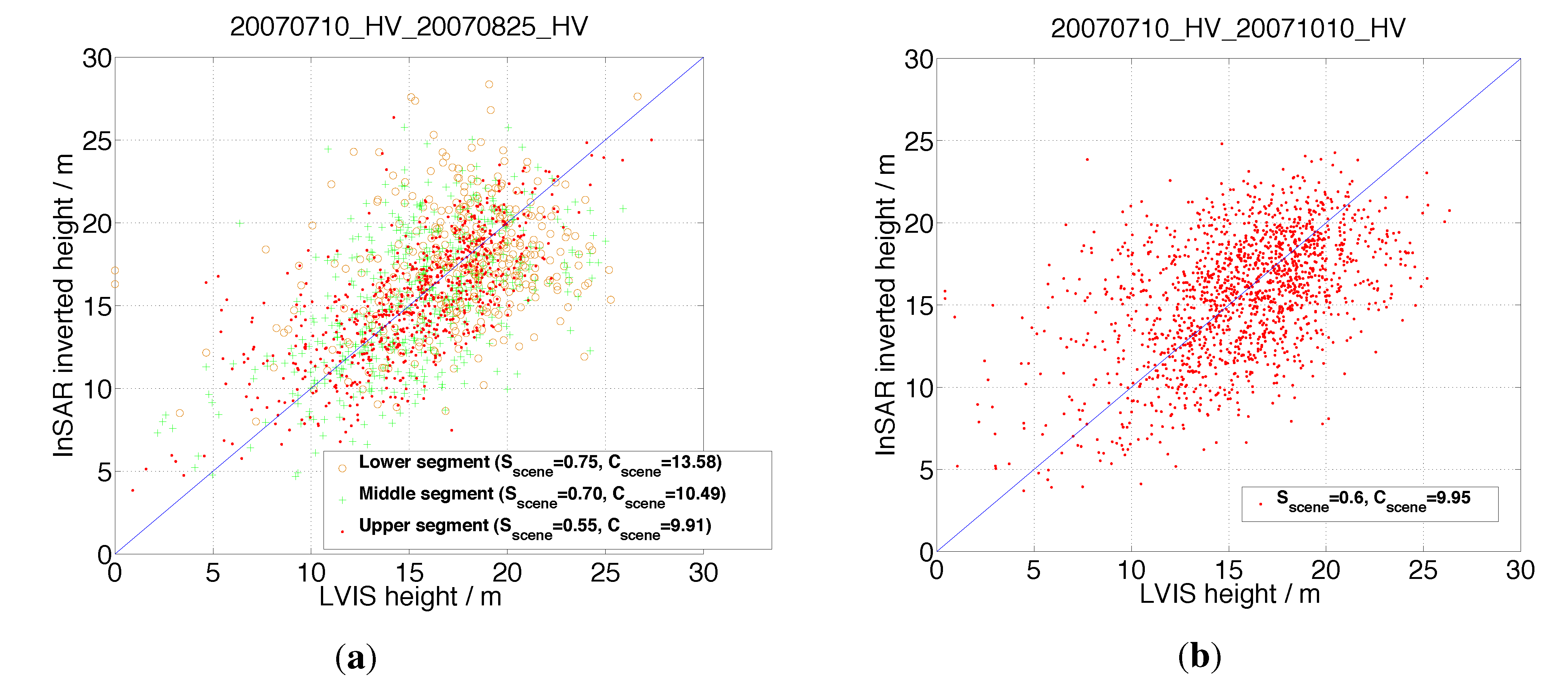
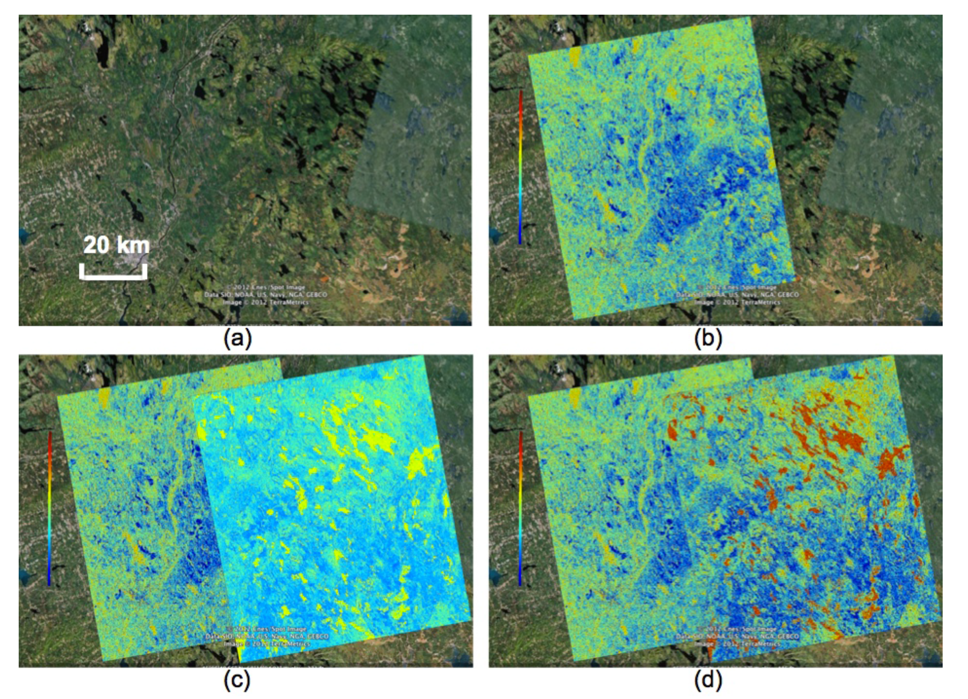
Section 5. The target-dependence of these parameters across a scene leads to RMSE < 4 m in the forest height estimation. Note importantly, this assumption only works under the conditions that the temporal decorrelation does not exhibit a spatially-varying gradient across the scene. When the temporal decorrelation has a strong gradient across the scene (e.g., see 
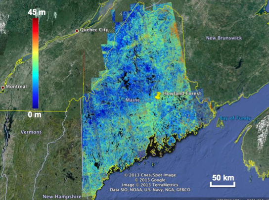
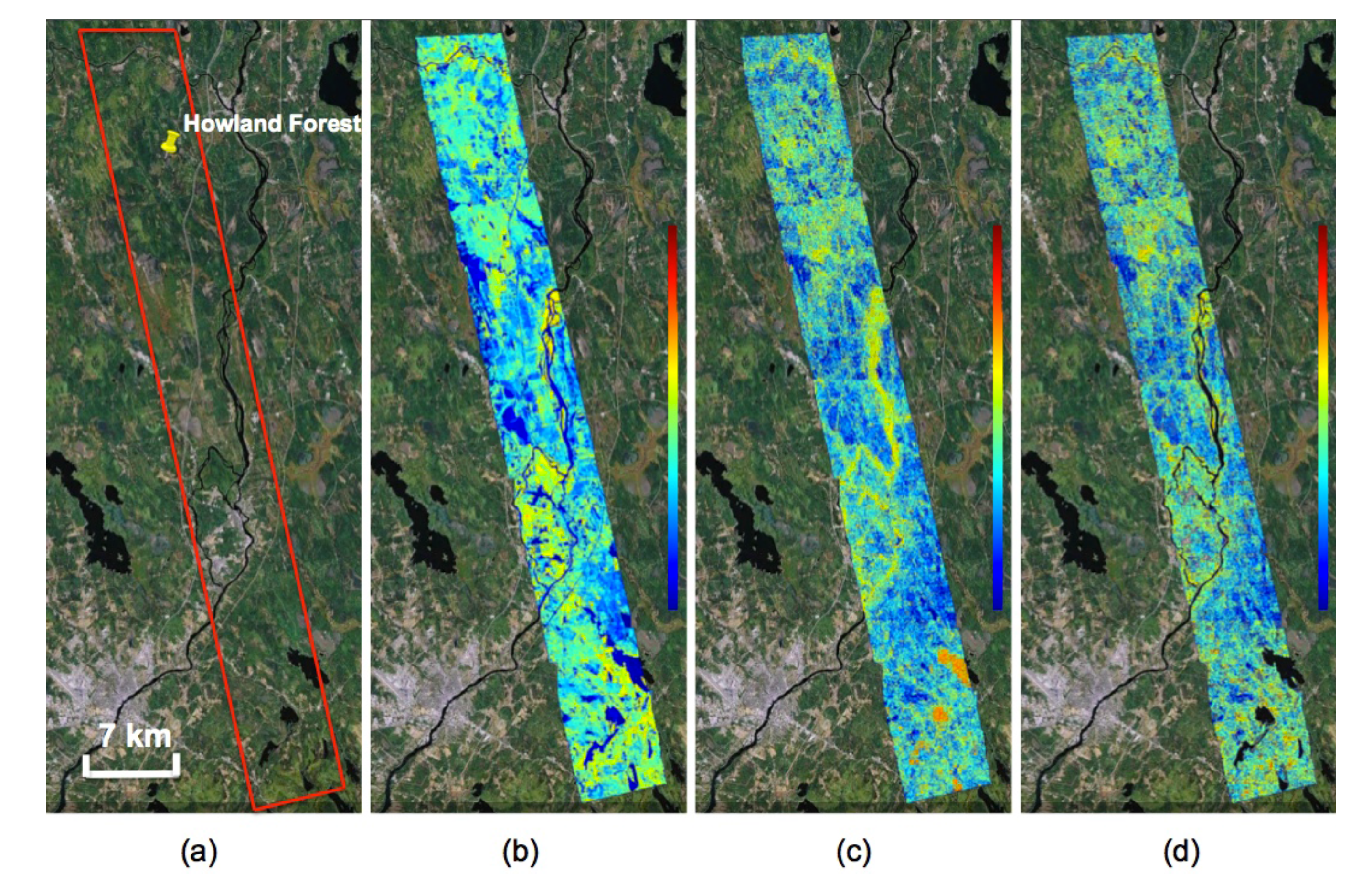
Figure 8a; primarily caused by nonuniform precipitation), the scene can be broken into smaller component parts, and in so much as ancillary measures of forest heights are available, these variations can be accounted for. In the case that the spatial variation of the model parameters is not desired, different time periods for the observations (with no precipitation occurring) can be chosen (as in Figure 8b).
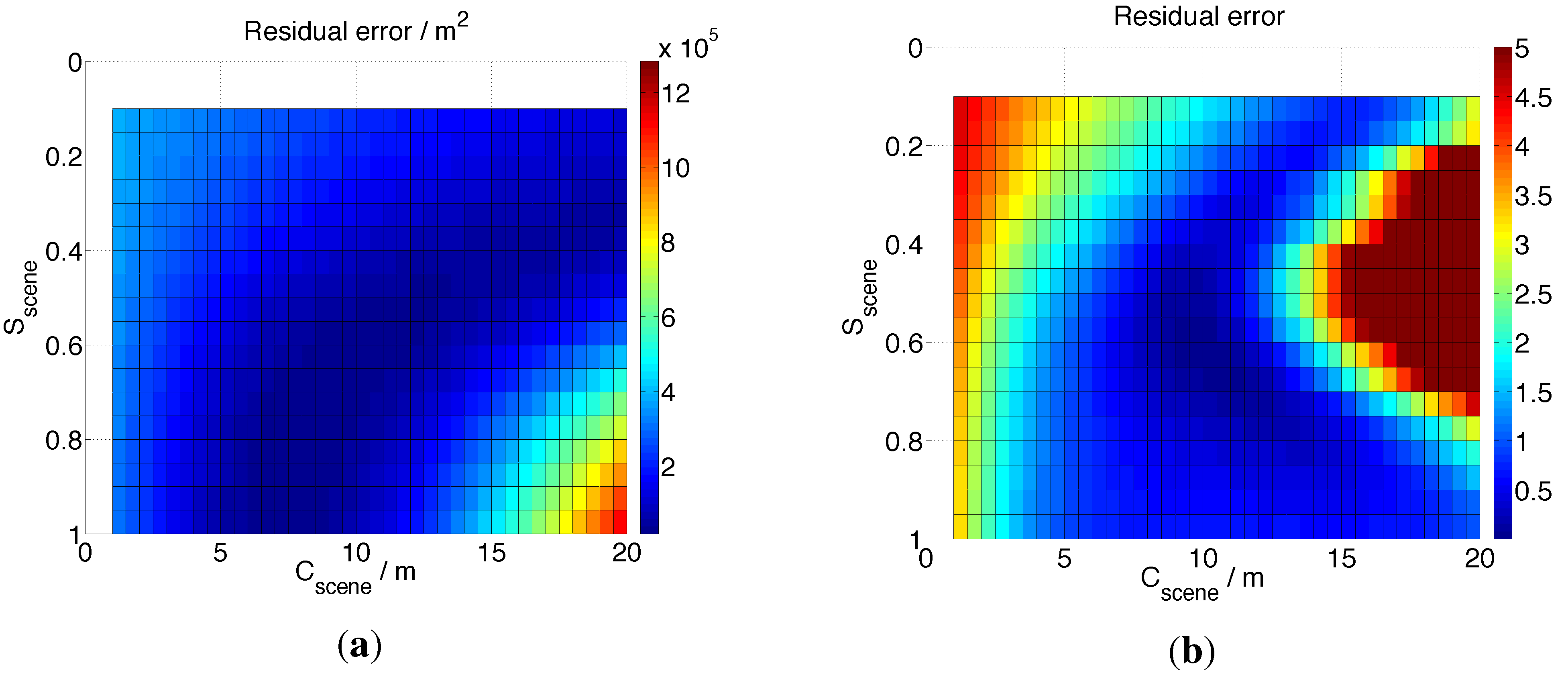
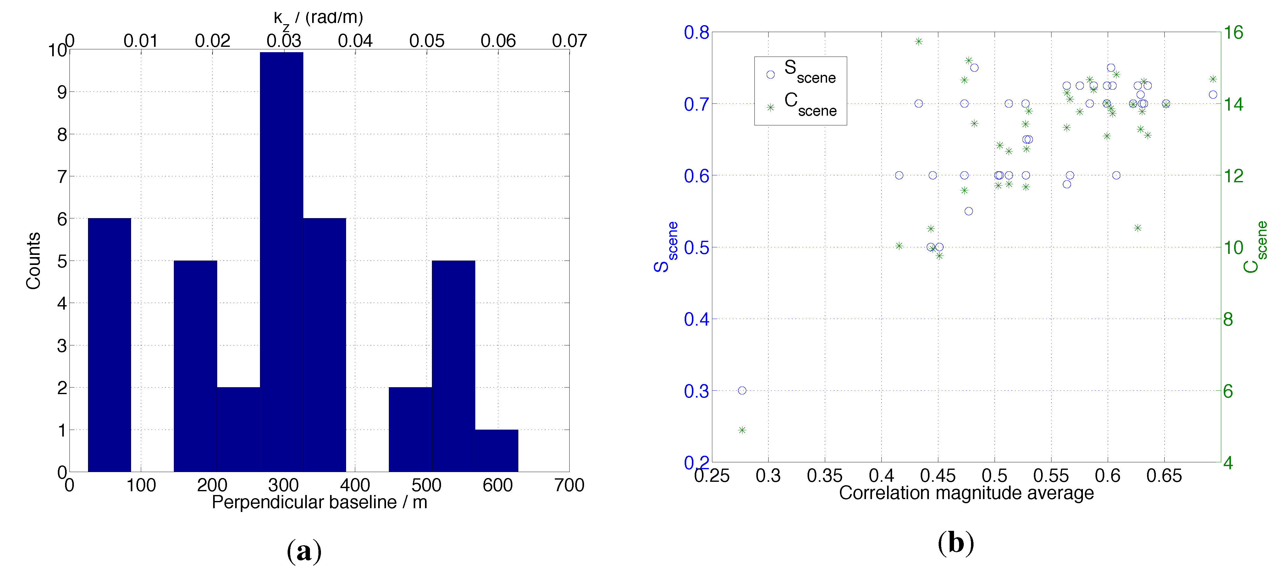
To provide more insight into the temporal decorrelation gradient observed in Figure 8a, a comparison can be made with ancillary observations of precipitation data that were collected from NOAA’s National Climate Data Center (NCDC; [20]) during the time period of the satellite passes. For the inversion shown in 
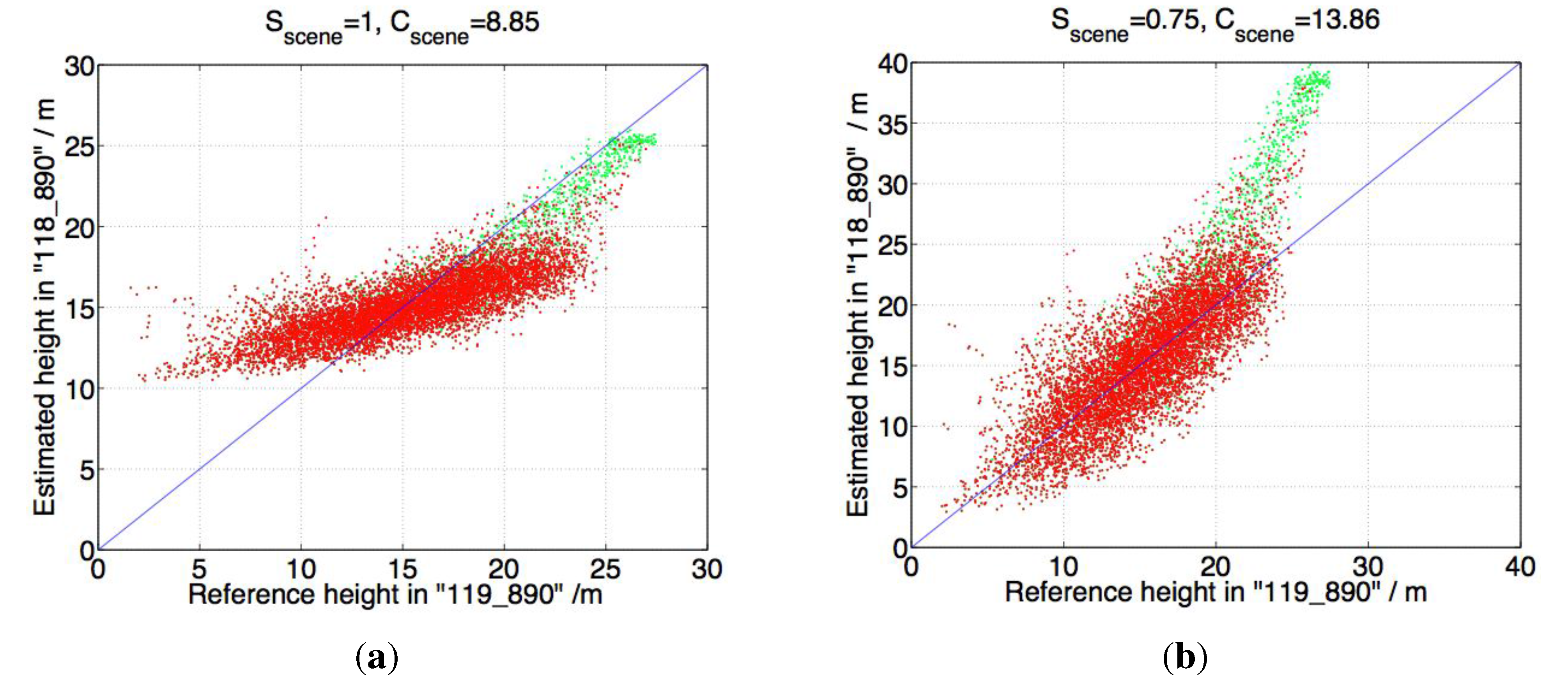
Figure 8a, it can be seen that the “upper” (i.e., northern) segment has smaller values of Sscene and Cscene than the “lower” (i.e., southern) portion. This implies that the weather conditions over the northern region were changing more compared to the southern region during the repeat period 07/10/2007–08/25/2007. These results were compared to the inversion shown in Figure 8b which used observations from 07/10/2007–10/10/2007, and can be characterized by a single set of temporal change parameters, implying that the weather conditions were uniform over the region.
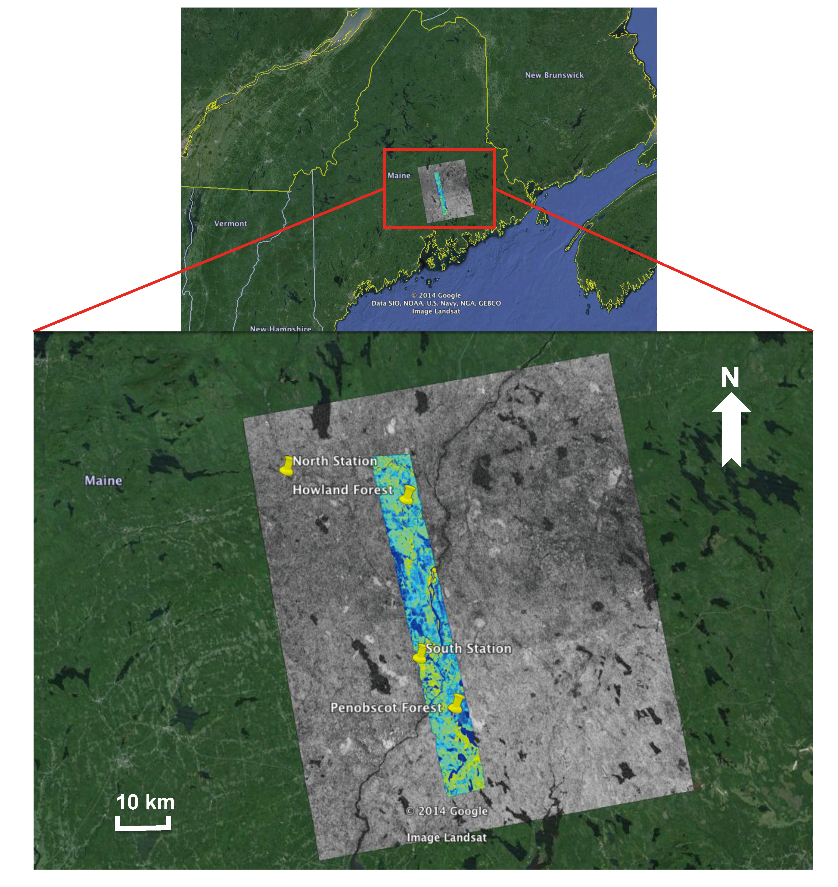
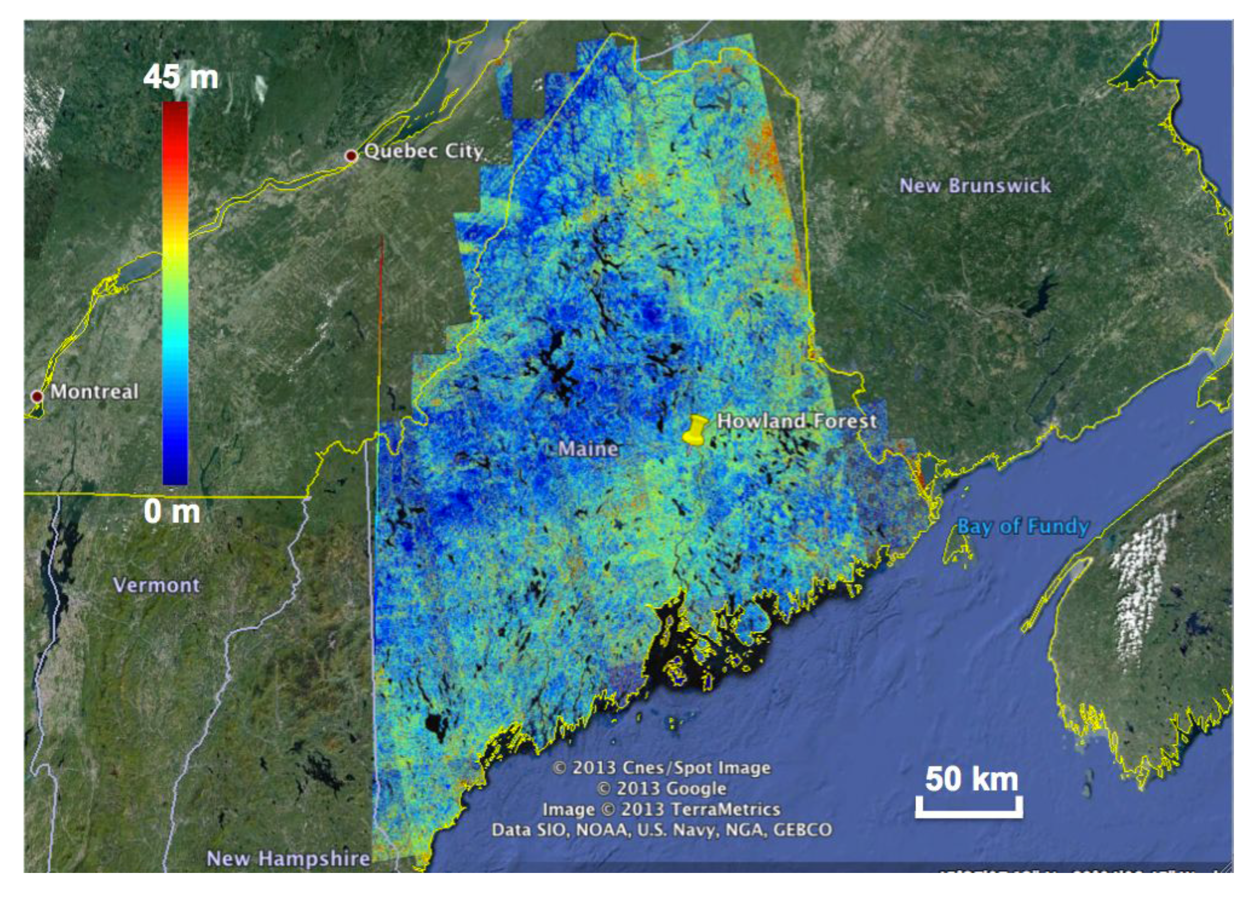
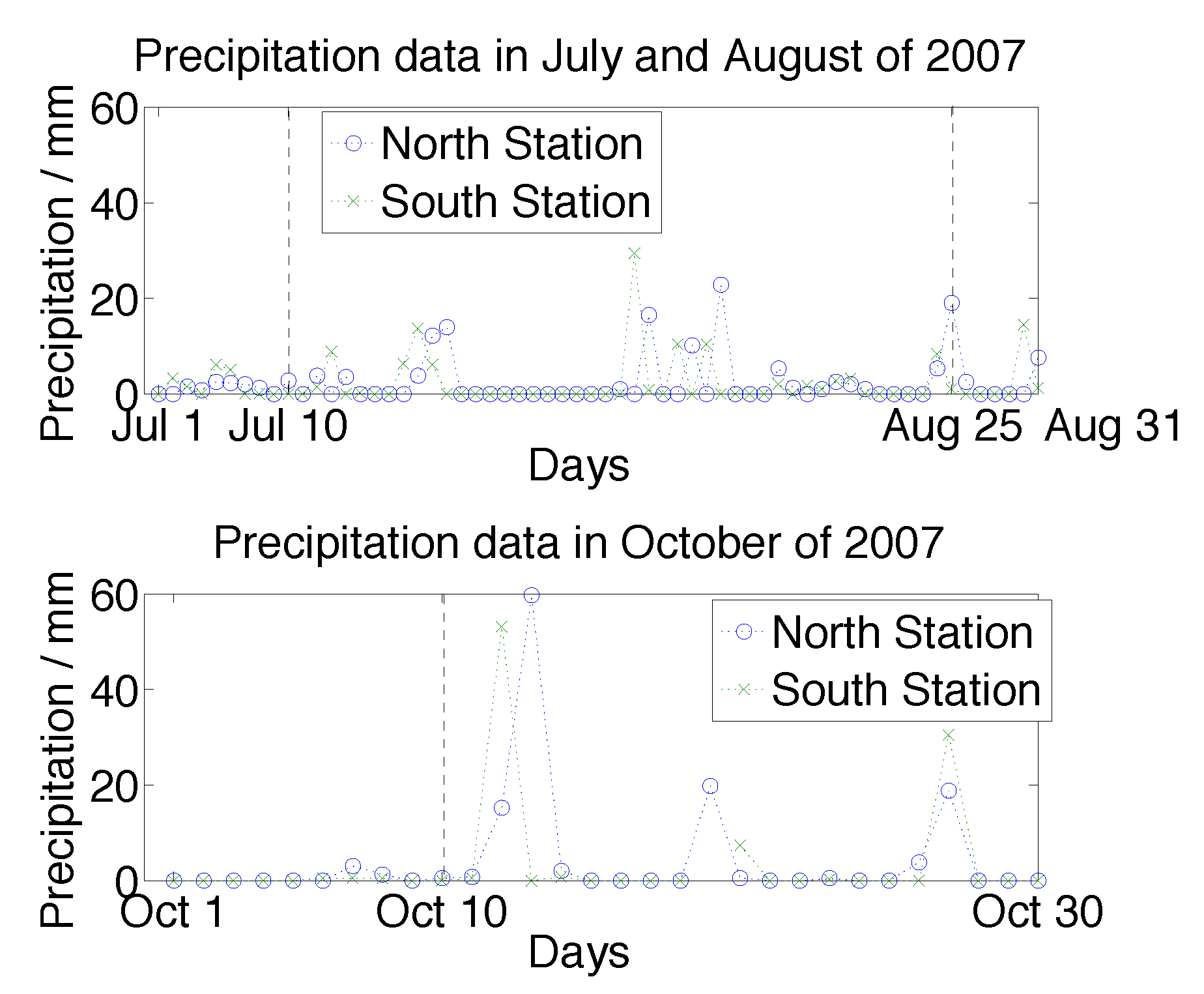
In Figure 5, the locations of two climate observing stations (marked as “North Station” and “South Station”) in central Maine are shown. The precipitation data associated with these two stations in July, August and October 2007 are given in Figure 14. The collection dates of the interferograms are indicated by vertical dashed lines. For interferogram 07/10/2007–08/25/2007, it can be seen that the precipitation for both north and south stations are similar on 07/10/2007, while the north station recorded a heavier rainfall on 08/25/2007 than the south station. In contrast, for interferogram 07/10/2007–10/10/2007, both north and south stations experienced similar level of precipitation on 07/10/2007 and 10/10/2007, hence providing evidence for the source of the temporal decorrelation gradient observed in Figure 8a, and not observed in Figure 8b.
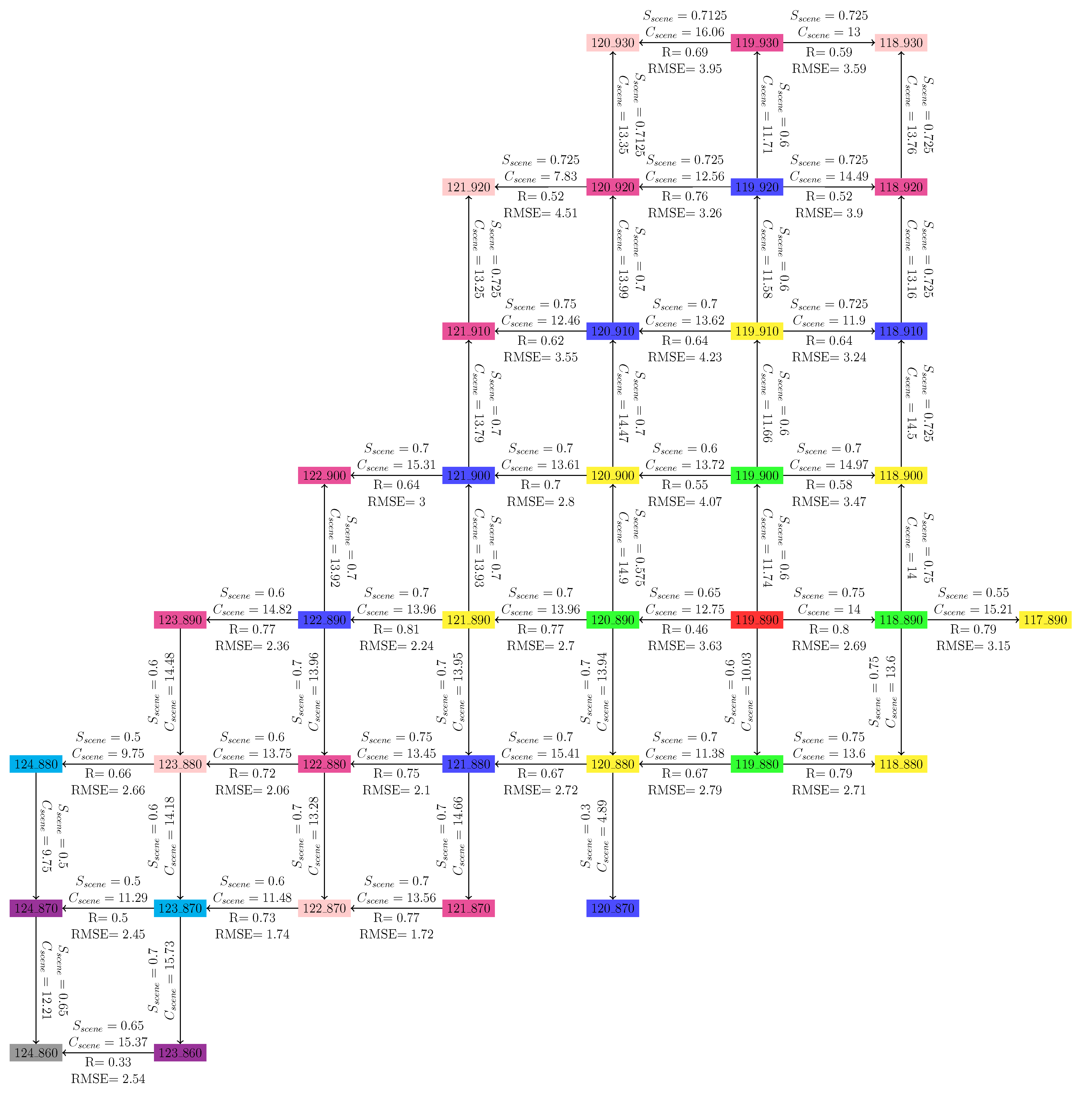
An alternative way to look at this homogeneity issue while performing the mosaicking task is through the overlapping regions from adjacent interferometric estimates of forest height. When there is a spatially-varying feature of the temporal change effects across the region, large errors are occurring and scenes should be replaced with alternate or new observations.
Another assumption that is made in enforcing a constant value for the parameter 
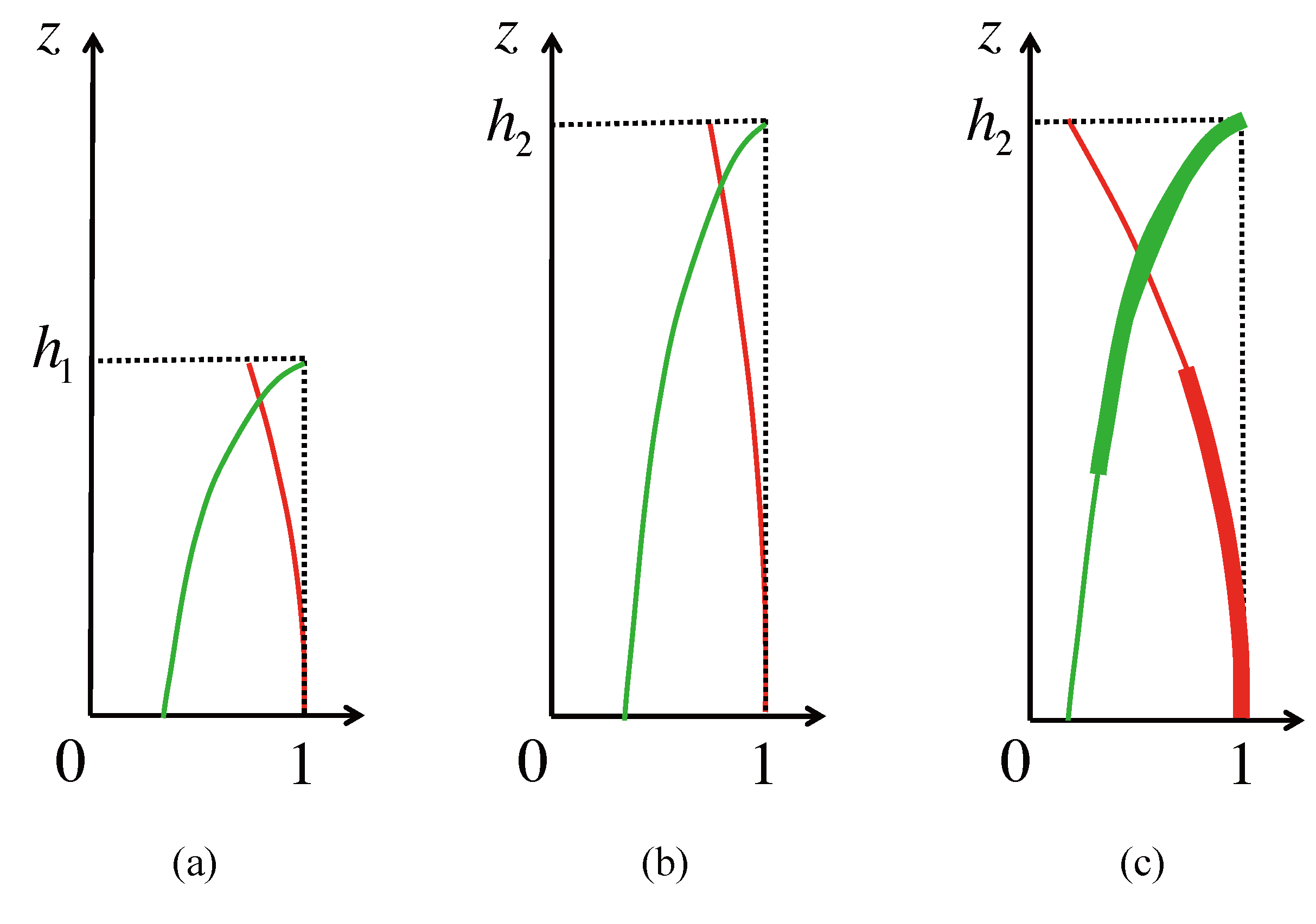
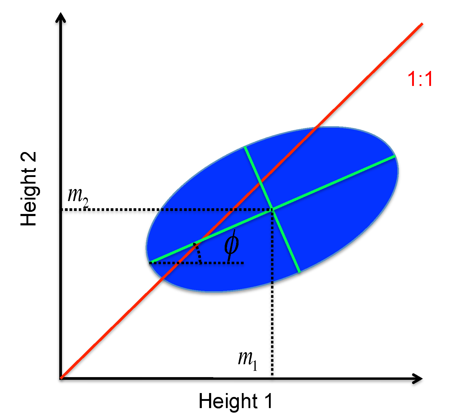
Cscene in deriving Equation (10) is that, all of the forests with different height values across the given scene have the scaled versions of extinction-weighted backscattering profile and height-dependent motion profile. To examine this assumption in more detail, the reader is referred to Figure 15 where a short forest stand of height h1 and a taller forest stand with height h2 (h2 = c · h1, where c is a scaling constant) are shown. Denoting the Gaussian motion profile in Equation (8) as, ρr(z), the mean-value theorem can be applied to Equation (8) for h1 and h2 such that
0 h i ρ r ( i ) ( z ) σ V ( i ) ( z ) d z 0 h i σ V ( i ) ( z ) d z = ρ r ( i ) ( ξ i )  for  i = 1 , 2
Mathematically, the choice of the mean value ξ depends on the functional forms of both σV(z) and ρr(z). By using a change of variables, it can be shown that if ρ r ( 2 ) ( z ) = ρ r ( 1 ) ( z c ) and σ V ( 2 ) ( z ) = σ V ( 1 ) ( z c ) then ξ2 = c · ξ1 or equivalently ξ 2 h 2 = ξ 1 h 1 . That is, when the extinction-weighted backscattering profile and the height-dependent motion profile of different forest stands are scaled versions of each other, the proportionality of the mean value with respect to the forest height is the same for all of the forest stands.
Figure 14. Precipitation data from NOAA’s National Climate Data Center in July, August and October 2007. The data was recorded at both north and south stations in central Maine. The collection dates of the corresponding interferograms are indicated by dashed lines.
Remotesensing 06 10252 g014
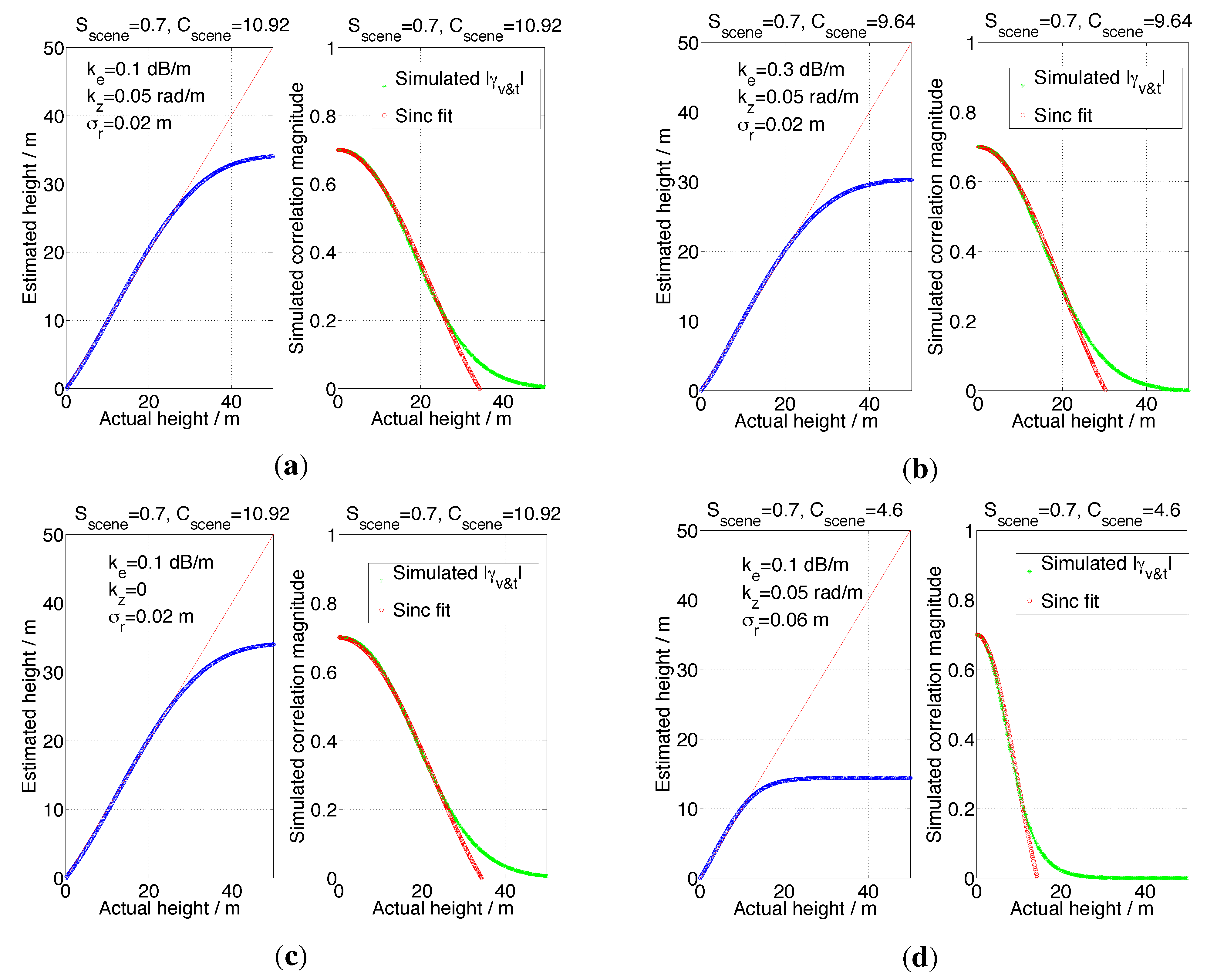
In most cases, however, this requirement is not strictly satisfied, as illustrated in Figure 15. Here, for forests with constant extinction coefficient and constant wind-induced motion level as assumed in Section 3.3 (e.g., Figure 4a), the profiles of σV(z) and ρr(z) are illustrated in Figure 15a,c for heights h1 and h2, respectively. However, in order to guarantee the same proportionality of the mean value, we would desire the profiles at height h2 are nothing more than scaled versions of the ones at height h1, i.e., Figure 15b. Therefore, the proportionality (denoted by α in Section 3.1) will have a perturbation for various forest heights in Figure 4a. For example, the standard deviation of α is calculated as 0.07, which in turn results in a standard deviation of 1.11 for Cscene through using Equation (11). In spite of this small perturbation of α (and thus Cscene), the overall fit as shown in Figure 4a is still quite good (RMSE = 0.25 m and R = 99.97% for heights under the saturation point). So far, we have seen that the requirement of the scaled versions of profiles for different heights could be weakly satisfied with small perturbation occurring but the overall quality of the fitting is still good.
Since we already considered constant wind-induced motion level in the mean sense, for the constant extinction coefficient as mentioned above and utilized in Section 3.3, we can still apply the same idea by considering its mean value across the whole scene. As seen from Figure 4b, the fitting parameter Cscene has a weak dependence on the extinction coefficient ke compared to the wind-induced motion level σr (Figure 4d). Therefore, if we can consider constant motion level in terms of its mean behavior, we can also safely treat the extinction coefficient in the same way, since the target-dependence of ke is expected to have a smaller effect on the fitting parameter Cscene than that due to σr.
Figure 15. Illustration of different functional forms of the extinction-weighted backscattering profile (normalized; “green” curve) and the height-dependent motion profile (“red” curve). (a) shows the profiles for a short forest stand at height h1, (b) shows the profiles that are scaled versions of (a) for a taller forest stand at height h2, while (c) shows the profiles for the taller forest stand at height h2 using the same functional forms of σV(z) (i.e., constant extinction coefficient) and ρr (z) (i.e., constant wind-induced motion level) as (a). Note the highlighted curve segments in (c) exactly correspond to the profiles in (a).
Remotesensing 06 10252 g015

Appendix B. Polarization-Dependence of the Forest Height Inversion Procedure

The forest height inversion procedure used in Figure 12 is based on Equation (7) which is a version of the correlation model (4), simplified by assuming that m = 0 for HV-pol data. For the more general case, where both µ, the ground-to-volume temporal decorrelation ratio due to dielectric change, and m, the ground-to-volume power ratio, are not trivial values (e.g., for the case of co-polarized transmit and receive channels), the contribution of ground scattering can be further investigated.
To understand these effects of undoing these assumptions, the general correlation model, Equation (4), is rewritten as
γv&t = Sscene · γ′v&m
with
γ v & m = γ v & m + µ m 1 + m
where µ and m will bias γ′v&m from γv&m.
To obtain the inverted forest height, Equation (10) is used to determine hv , while we maintain the same Sscene and Cscene as in the simplified model (see Figure 4a) but γv&t is replaced by Equation (19) while calculating the simulated correlation magnitude. When m = 0, this reduces to the simplified model. 
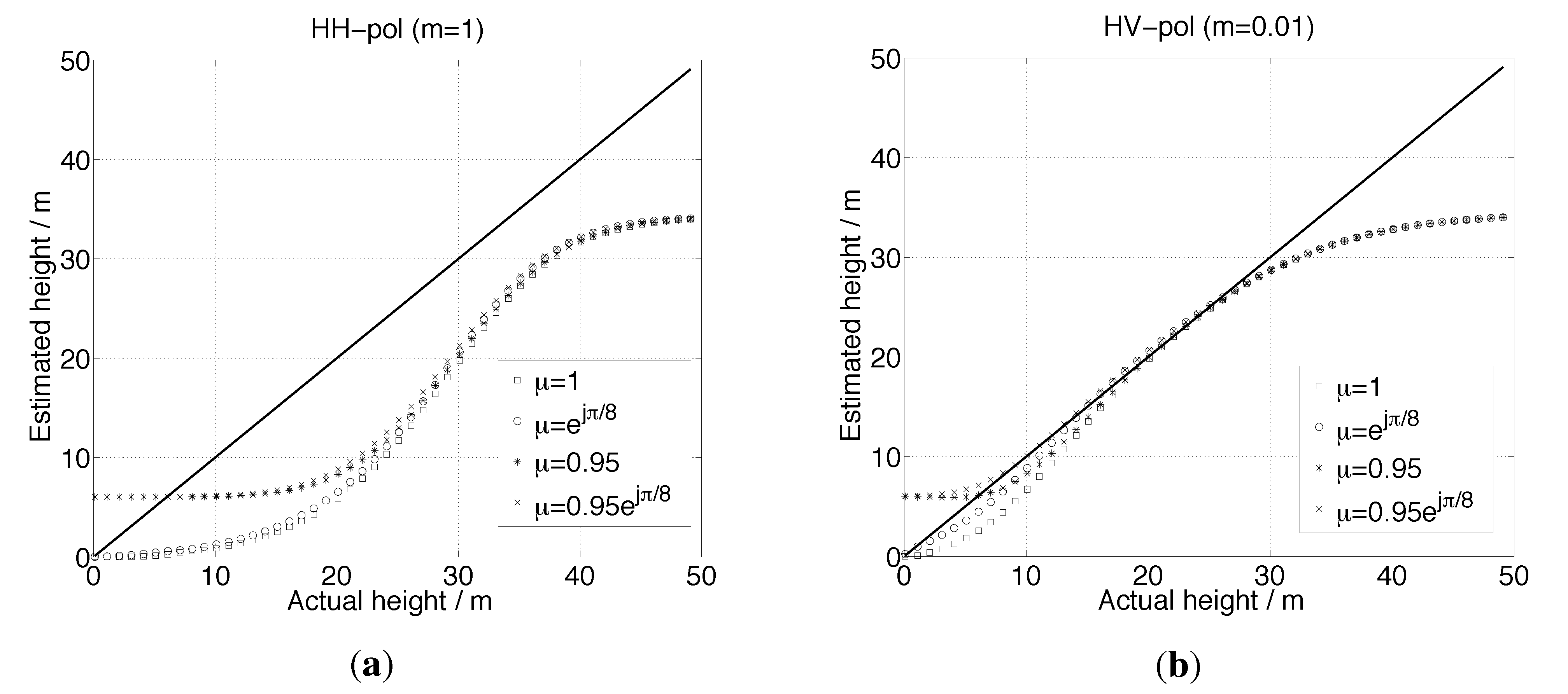
Figure 16 demonstrates the simulated inversion results when m = 1 (large m, or HH-pol data; Figure 4a) and m = 0.01 (Figure 4b for HV-pol), where the value of m is referenced to a 30 m tall canopy as in [3]. Both subplots demonstrate the inversion model performance with µ = 1 ,   e j π 8 ,   0.95 ,   0.95 e j π 8 allowing µ to have magnitude and/or phase bias in comparison with µ = 1.
From the plots shown in Figure 16 it can be seen that significant contributions from ground scattering (from the HH-polarized case in (a)) create a non-linear relationship between actual and estimated heights, whereas for the HV-pol data (small m), the model works well under almost all values of heights. For the small m case, differences between the simulated and estimated heights only exist at the short and very tall extremes of the inversion. It is for this reason that a preference is given for the use of cross-polarized data in the inversion, a fact that has been borne out in observational data as well.
Figure 16. Simulated forest height inversion results using (a) m = 1 (HH-pol) and (b) m = 0.01 (HV-pol). The instrumental and forest parameters are the same as in Figure 4a, so are the fitting parameters (Sscene and Cscene). Results are shown with µ = 1 ,   e j π 8 ,   0.95 ,   0.95 e j π 8 .
Remotesensing 06 10252 g016
Although it would be better to make a rigorous mathematical proof in order to validate this assumption, we note the above simulation method (e.g., Figure 16) is sufficient at this stage. The purpose of this assumption is to show when m 0, bias exists in the inverted forest height. However, as long as m is small, this only affects the lower end of the height range (e.g., short vegetation and ground), which can be tolerated if m is small enough, or alternatively can be masked out through the use of a forest/non-forest map since there is usually extra temporal decorrelation causing overestimation of the low heights. The fact of HV-polarized data with m being small enough in the present work has been validated both by the simulation results (Figure 16) and the experimental results ( and ).
In the above simulation, an extinction coefficient of ke = 0.1 dB/m (less than the values used in [3,9]) is used to characterize a sparse forest at L-band. If a dense forest is studied with a greater ke = 0.3 dB/m (as in [9]), the bias in the lower end of the height range will become much less pronounced, i.e., the model performs much better. However, if a very spare forest is examined, the extinction effect will be so small that the ground-to-volume ratio will be huge even for a 30 m tall canopy. The inversion result for the HV-polarized data in this case will look very much like the HH-polarized data in the above simulation (Figure 16a). The forest heights will thus be severely underestimated, however, since the forest is very sparse, the mean ground truth height will also be very small (close to the ground). As this paper deals with the forest height through averaging a large area (not the maximum height), the biased difference between the estimated and ground truth heights can be tolerated for very sparse forests.
In the presence of temporal decorrelation, it is important to note that Sscene, m and µ will be polarization-dependent. Therefore, the PolInSAR version [6,15] of this problem will have additional unknowns when temporal decorrelation is expected to play a role in the observations, and thus the inversion becomes an underdetermined problem [13]. While sophisticated techniques (e.g., adapting PolInSAR methods to accommodate Equation (4)) might lead to more accurate inversion, the simplified inversion model shown here (based on HV-pol data only) has been shown to generate meaningful results from repeat-pass InSAR correlation measurements with long repeat periods. Such algorithms thus are important tools for making use of accumulated data from the JERS-1, ALOS-1 & -2 data sets, as well as the planned DESDynI-R (now called NISAR) mission.

Appendix C. Effective Range of kz for this Work and the Small-kz Assumption

Generally speaking, an InSAR correlation magnitude varies with the kz value as indicated in Figure 6 and in [11] (under unfrozen conditions). In this appendix, the range of kz values that can be used for this inversion model are explored. In order to do this it is useful to differentiate the decorrelation effects from the variety of sources, as they change with respect to kz. Although these decorrelation components are demonstrated here as simulation results, as mentioned in Section 3.3, these simulation parameters are intentionally chosen to be such in order to mimic the experimental results in Section 5. To create an example, a 20 m tall canopy is used and the kz-dependence of various correlation components is illustrated in Figure 17 with the same forest parameters as in Figure 4a, and using a viewing geometry consistent with ALOS/PALSAR.
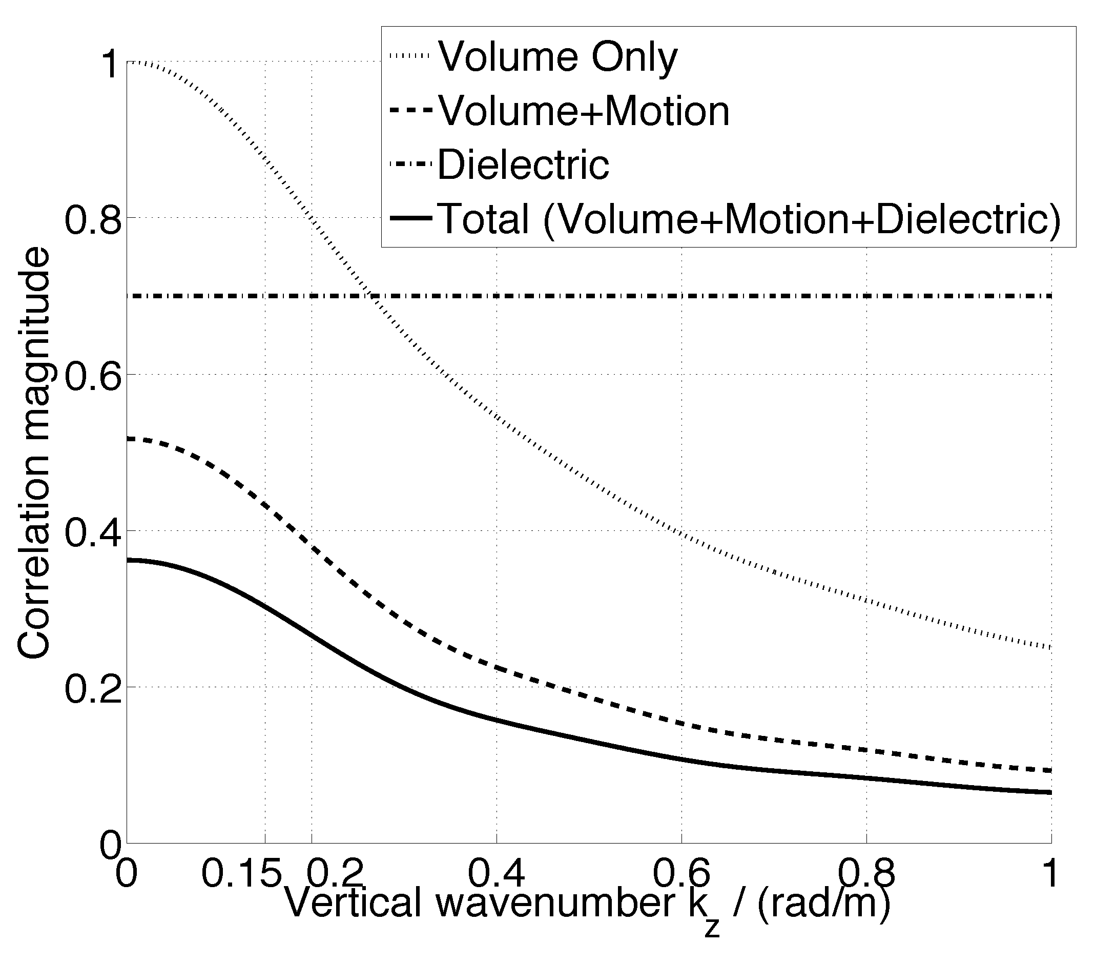
In Figure 17, the “Volume Only” contribution is from volume scattering and no motion, “Dielectric” is the model for the loss of correlation magnitude due to dielectric changes in the volume (a constant factor that manifests itself in the model constant, Sscene), “Volume+Motion” is the magnitude of the coupled correlation component due to volume scattering and random motion (|γv&m|, as in Equation (5)), and “Total (Volume+Motion+Dielectric)” is the combined correlation magnitude from all volume scattering and temporal changes, |γv&t|. In this example, it is assumed that the geometric decorrelation has been compensated for and that the thermal noise correlation is negligible for 20 m tall canopy.
From Figure 17, it can be seen that as the vertical wavenumber increases, the total observed correlation decreases, as expected (which agrees with the observations in Figure 6), and that the combined effect of all correlations can make this total correlation quite low (below a value of 0.3). This has the effect of making the correlation magnitude difficult to measure [16], and also is an indication of a loss of information in the observation itself. For these reasons, for any model and subsequent inversion used, it is important to use those correlations that have the highest values, such as those shown in Figure 6. Because of the variety of sources of decorrelation when a 46 day repeat-period is introduced (i.e., both dielectric and motion changes occur in the target), those observations with the shortest baselines will have the largest correlations, and hence information content. So long as there is a height-dependent sensitivity of the decorrelation on these changes (e.g., [8,9]), a signature will exist that can be exploited to estimate forest height.
Figure 17. Illustration of the kz-dependence for all of the correlation components involved in the current work by utilizing ALOS’s viewing geometry over a 20 m tall canopy. The forest and temporal change parameters are chosen as in Figure 4a. The effective range of kz for this study is kz < 0.15 rad/m.
Remotesensing 06 10252 g017
The effect of changing the vertical wavenumber, kz, from zero to some other value, under these circumstances will lead to a graceful degradation in the model’s performance, because the effect of this larger wavenumber will only be to decrease the correlation. Note that when kz 0, a non-zero value of kz will be included in the model via the scene-wide parameter, Cscene, derived in Equation (7) through Equation (11). While in that derivation, the vertical wavenumber was assumed to be zero, a non-zero but small value of that parameter will have the effect of scaling the argument of the exponential function given in Equation (9), or equivalently, scaling the argument of the sinc function used in Equation (10). In other words, the fitting parameter Cscene will be 
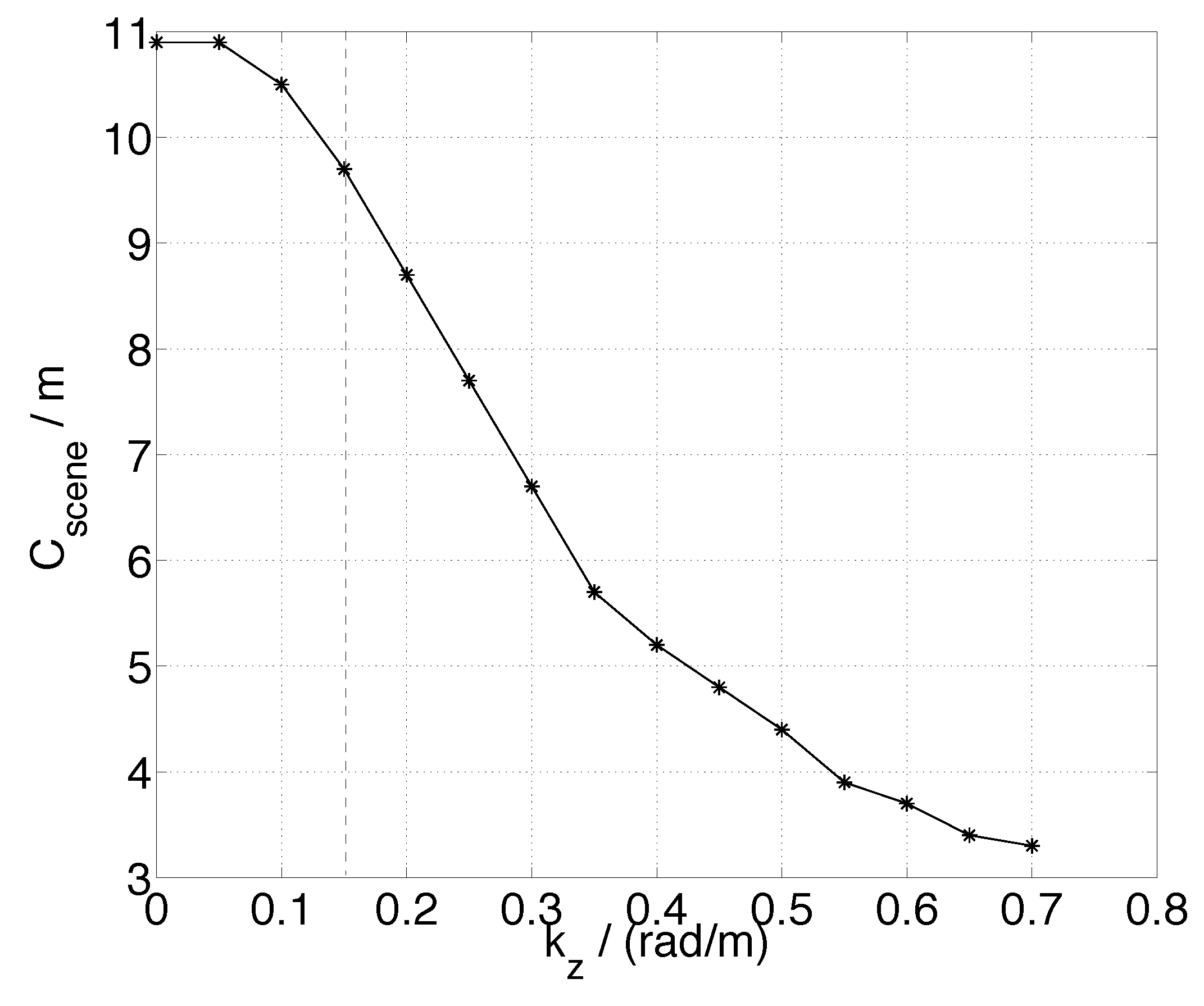
kz -dependent in order to compensate the model degradation. This effect can be better illustrated by Figure 18, which shows the fitted parameter Cscene as a function of kz with other simulation parameters fixed as in Figure 4a. As mentioned in Section 3.1, the value πCscene represents the invertible range of forest height through using the simplified inversion model (“sinc” relationship) with fitting parameters Sscene and Cscene. If Cscene becomes very small (e.g., <5 m as seen in Figure 18), this simplified inversion approach will be insufficient to characterize the height variation of natural forests under the presence of correlation measurement uncertainty. Note for the small kz values (i.e., kz < 0.15 rad/m and preferably < 0.05 rad/m as stated above), the value of Cscene is only slightly changed, which is in agreement with Figure 4a, where kz = 0.05 rad/m and Figure 4c, where kz = 0 rad/m. The reason for this can be seen in the effect of kz on the total decorrelation curve shown in Figure 17, where the behavior of the curve for small values of kz is at its peak, and relatively unchanged for values of kz < 0.15 rad/m (as indicated by the vertical dotted line included in Figure 17), which serves as the effective range of kz for this study. Therefore, we have demonstrated that for any non-zero small kz , this simplified inversion model (i.e., the sinc relationship as in Equation (10)) can always work well with Cscene being weakly dependent on kz (in comparison to Equation (11) where kz was neglected), which is referred to as the “small-kz assumption” in this study.
Figure 18. The kz-dependence of the inversion model degradation. Particularly, the fitted parameter Cscene is shown as a function of kz with πCscene related to the invertible range of forest height characterizing the model performance. The smaller Cscene, the worse model performance. The forest and temporal change parameters in this simulation are set to be the same as Figure 4a. The case where kz = 0.15 rad/m (i.e., boundary of the effective range for small kz in this study) is indicated by a vertical dashed line.
Remotesensing 06 10252 g018

Conflicts of Interest

The authors declare no conflict of interest.

References

  1. Goetz, S. The lost promise of DESDynI. Remote Sens. Environ. 2011, 115, 2751. [Google Scholar] [CrossRef]
  2. Treuhaft, R.; Siqueira, P. Vertical structure of vegetated land surfaces from interferometric and polarimetric radar. Radio Sci. 2000, 35, 141–177. [Google Scholar] [CrossRef]
  3. Papathanassiou, K.; Cloude, S. Single-baseline polarimetric SAR interferometry. IEEE Trans. Geosci. Remote Sens. 2001, 39, 2352–2363. [Google Scholar] [CrossRef]
  4. Ahmed, R.; Siqueira, P.; Hensley, S.; Chapman, B.; Bergen, K. A survey of temporal decorrelation from spaceborne L-Band repeat-pass InSAR. Remote Sens. Environ. 2011, 115, 2887–2896. [Google Scholar] [CrossRef]
  5. Simard, M.; Hensley, S.; Lavalle, M.; Dubayah, R.; Pinto, N.; Hofton, M. An empirical assessment of temporal decorrelation using the uninhabited aerial vehicle synthetic aperture radar over forested landscapes. Remote Sens. 2012, 4, 975–986. [Google Scholar] [CrossRef]
  6. Lee, S.; Kugler, F.; Papathanassiou, K.; Hajnsek, I. cation and compensation of temporal decorrelation effects in polarimetric SAR interferometry. In Proceedings of the 2012 IEEE International Geoscience and Remote Sensing Symposium (IGARSS), Munich, Germany, 22–27 July 2012; pp. 3106–3109.
  7. Lee, S.K.; Kugler, F.; Papathanassiou, K.P.; Hajnsek, I. Quantification of temporal decorrelation effects at L-band for polarimetric SAR interferometry applications. IEEE J. Sel. Top. Appl. Earth Obs. Remote Sens. 2013, 6, 1351–1367. [Google Scholar] [CrossRef]
  8. Askne, J.I.; Dammert, P.B.; Ulander, L.M.; Smith, G. C-band repeat-pass interferometric SAR observations of the forest. IEEE Trans. Geosci. Remote Sens. 1997, 35, 25–35. [Google Scholar] [CrossRef]
  9. Lavalle, M.; Simard, M.; Hensley, S. A temporal decorrelation model for polarimetric radar interferometers. IEEE Trans. Geosci. Remote Sens. 2012, 50, 2880–2888. [Google Scholar] [CrossRef]
  10. Askne, J.; Santoro, M.; Smith, G.; Fransson, J.E. Multitemporal repeat-pass SAR interferometry of boreal forests. IEEE Trans. Geosci. Remote Sens. 2003, 41, 1540–1550. [Google Scholar] [CrossRef]
  11. Thiel, C.; Schmullius, C. Investigating ALOS PALSAR interferometric coherence in central Siberia at unfrozen and frozen conditions: Implications for forest growing stock volume estimation. Can. J. Remote Sens. 2013, 39, 232–250. [Google Scholar] [CrossRef]
  12. Hajnsek, I.; Kugler, F.; Lee, S.; Papathanassiou, K. Tropical-forest-parameter estimation by means of Pol-InSAR: The INDREX-II campaign. IEEE Trans. Geosci. Remote Sens. 2009, 47, 481–493. [Google Scholar] [CrossRef]
  13. Papathanassiou, K.; Cloude, S.R. effect of temporal decorrelation on the inversion of forest parameters from PoI-InSAR data. In. In Proceedings of the International Geoscience and Remote Sensing Symposium,, Toulouse, France, 21–25 July 2003.
  14. Lavalle, M.; Hensley, S. onstration of repeat-pass POLINSAR using UAVSAR: The RMOG model. In Proceedings of the 2012 IEEE International Geoscience and Remote Sensing Symposium (IGARSS), Munich, Germany, 22–27 July 2012; pp. 5876–5879.
  15. Cloude, S.; Papathanassiou, K. Three-stage inversion process for polarimetric SAR interferometry. IEE Proc.-Radar Sonar Navig. 2003, 150, 125–134. [Google Scholar] [CrossRef]
  16. Touzi, R.; Lopes, A.; Bruniquel, J.; Vachon, P. Coherence estimation for SAR imagery. IEEE Trans. Geosci. Remote Sens. 1999, 37, 135–149. [Google Scholar] [CrossRef]
  17. Cloude, S.R. Polarization coherence tomography. Radio Sci. 2006, 41. [Google Scholar] [CrossRef]
  18. Moon, T.K.; Stirling, W.C. Mathematical Methods and Algorithms for Signal Processing; Prentice Hall: New York, NY, USA, 2000. [Google Scholar]
  19. Heath, M.T. Scientific Computing: An Introductory Survey; The McGraw-Hill Companies Inc.: New York, NY, USA, 2002. [Google Scholar]
  20. NOAA’s National Climatic Data Center. Available online: http://ncdc.noaa.gov (accessed on 22 October 2014).
  21. Hollinger, D.; Goltz, S.; Davidson, E.; Lee, J.; Tu, K.; Valentine, H. Seasonal patterns and environmental control of carbon dioxide and water vapour exchange in an ecotonal boreal forest. Glob. Chang. Biol. 1999, 5, 891–902. [Google Scholar] [CrossRef]
  22. Sendak, P.E.; Brissette, J.C.; Frank, R.M. Silviculture affects composition, growth, and yield in mixed northern conifers: 40-year results from the Penobscot Experimental Forest. Can. J. For. Res. 2003, 33, 2116–2128. [Google Scholar] [CrossRef]
  23. Blair, J.; Rabine, D.; Hofton, M. The laser vegetation imaging sensor: A medium-altitude, digitisation-only, airborne laser altimeter for mapping vegetation and topography. ISPRS J. Photogramm. Remote Sens. 1999, 54, 115–122. [Google Scholar] [CrossRef]
  24. Shimada, M.; Isoguchi, O.; Tadono, T.; Isono, K. PALSAR radiometric and geometric calibration. IEEE Trans. Geosci. Remote Sens. 2009, 47, 3915–3932. [Google Scholar] [CrossRef]
  25. Rosenqvist, A.; Shimada, M.; Ito, N.; Watanabe, M. ALOS PALSAR: A pathfinder mission for global-scale monitoring of the environment. IEEE Trans. Geosci. Remote Sens. 2007, 45, 3307–3316. [Google Scholar] [CrossRef]
  26. Werner, C.; Wegmüller, U.; Strozzi, T.; Wiesmann, A.; Santoro, M. R multi-mode interferometric processing. In Proceedings of the 1st Joint PI Symposium of ALOS Data Nodes, Kyoto, Japan, 19–23 November 2007; pp. 19–23.
  27. Gatelli, F.; Guamieri, A.M.; Parizzi, F.; Pasquali, P.; Prati, C.; Rocca, F. The wavenumber shift in SAR interferometry. IEEE Trans. Geosci. Remote Sens. 1994, 32, 855–865. [Google Scholar] [CrossRef]
  28. Schwabisch, M.; Geudtner, D. Improvement of phase and coherence map quality using azimuth prefiltering: Examples from ERS-1 and X-SAR. In Proceedings of the IEEE International Geoscience and Remote Sensing Symposium, IGARSS’95, Florence, Italy, 10–14 July 1995; Volume 1, pp. 205–207.
  29. Zebker, H.A.; Villasenor, J. Decorrelation in interferometric radar echoes. IEEE Trans. Geosci. Remote Sens. 1992, 30, 950–959. [Google Scholar] [CrossRef]
  30. Fry, J.; Xian, G.; Jin, S.; Dewitz, J.; Homer, C.; Yang, L.; Barnes, C.; Herold, N.; Wickham, J. Completion of the 2006 national land cover database for the counterminous United States. Photogramm. Eng. Remote Sens. 2011, 77, 858–864. [Google Scholar]
  31. Siqueira, P.; Hensley, S.; Shaffer, S.; Hess, L.; McGarragh, G.; Chapman, B.; Freeman, A. A continental-scale mosaic of the Amazon Basin using JERS-1 SAR. IEEE Trans. Geosci. Remote Sens. 2000, 38, 2638–2644. [Google Scholar] [CrossRef]

