Retrieval of Particle Scattering Coefficients and Concentrations by Genetic Algorithms in Stratified Lake Water

Abstract
: We retrieved the mass-specific scattering coefficient b*sm(λ) = 0.60·(λ/650)−1.82 of the inhomogeneous and optically complex water column of eastern Lake Constance in May 2012. In-situ measured and modelled remote-sensing reflectance Rrs(λ) were matched via a parameter search procedure using genetic algorithms. The optical modelling consisted of solving the azimuthally-averaged Radiative Transfer Equation, forced with in-situ suspended matter concentration (sm) data. b*sm(λ) was univocally determined at red wavelengths. In contrast, we encountered unresolved spectral ambiguity at blue wavelengths due to the absence of organic absorption in our dataset. Despite this, a surprisingly good sm retrieval regression is achieved (R2 > 0.95 with respect to independent data) using our b*sm(λ). Acquisition of accurate inherent optical properties in future field campaigns is needed to verify the estimated b*sm(λ) and related assumptions.1. Introduction
Remote sensing of inland water quality is receiving increased attention in recent years in light of the emerging water crisis and the need for enhanced water quality monitoring [1–4]. Standard water quality parameters (WQPs) retrieved by remote sensing are mass concentrations of chlorophyll-a (chl), suspended matter (sm), and yellow substance (y; also referred to as gelbstoff or coloured dissolved organic matter (CDOM), quantified by means of their light absorption at 440 nm [5]). The inherent optical properties (IOPs) are the responses of water and its constituents to an incident collimated light source, i.e., absorption and scattering coefficients (the latter, angularly resolved, is the volume scattering function). IOPs are useful because they vary with the concentration of each WQP through the specific inherent optical properties (SIOPs) [6]. In particular, the mass-specific absorption and scattering coefficients of suspended matter are obtained by: a*sm(λ) = asm(λ)/sm, and b*sm(λ) = bsm(λ)/sm. SIOPs are used as ancillary knowledge to obtain the actual WQPs from remotely-retrieved IOPs. The spatial variability seawater SIOPs has been described by many investigations [7–12]. Seasonal variability has also been reported [13]. However, little is known about SIOPs in inland waters and the few measurements that have been performed are not directly transferable to other lake systems.
The spectro-radiometric quantities (radiances and irradiances) are determined by the IOPs and the ambient conditions through radiative transfer forward models. Early models ignored the vertical variation of WQPs, assuming a vertically homogeneous surface water layer [14]. However, the vertical distribution of WQPs is oftentimes non-uniform not only in oceanic chlorophyll-dominated waters [15] and coastal turbid waters [16], but especially so in inland waters [17]. Bélanger et al. [18] concluded recently that appropriate optical closure between measured and modelled radiometric quantities require the consideration of the vertical structure of near-surface IOPs.
Inversion procedures retrieve IOPs from spectro-radiometric quantities. Such procedures can be based on solving the Radiative Transfer Equation (RTE) [19] or making approximations if the computational time is limiting [20]. In the cases where a closed algebraic expression for the IOPs is not possible, minimization routines are used. Global optimization methods provide the absolute minimum of a certain goal function defined over all possible values of the unknown parameters. Among them, genetic algorithms (GA; [21]) are particularly useful for dealing with complex problems and a large number of unknowns [22]. GA have been employed in numerous fields of science and technology and are especially popular in computer-aided design, where GA search for the set of parameters that leads to the best performance based on the design criteria [23]. An important advantage of GA is that they make no assumptions about the structure of the modelled system as it is treated as a black-box. During model calibration, GA search for the optimal set of model parameters to minimize the deviation between the model output and the desired result [24].
In remote sensing, GA are widely used in land-cover classification [25–27] and retrieval of vegetation parameters [28–30]. However, despite their proven performance, GA have been less used in the context of water colour and corresponding quality. Chami and Robilliard [31] used GA to invert oceanic constituents from simulated data for case 1 and case 2 waters. Haigang et al. [32] described the performance in optically deep waters. Chang et al. [33] coupled GA to a semi-analytical algorithm with application to MODIS-Aqua imagery. Chen et al. [34] used GA to build an empirical equation with optimal coefficients to retrieve chl in a mesotrophic reservoir based on Landsat imagery. Chang-Chun et al. [35] used GA and a semi-analytical algorithm to evaluate the concentration of two different phytoplankton species in a eutrophic lake. Song et al. [36] combined GA and partial least-squares to build an empirical algorithm for the retrieval of chl in turbid waters.
In this study, we use GA to estimate an appropriate b*sm(λ) for Eastern Lake Constance using Rrs(λ) and sm(z) as model inputs. The approach is driven by the lack of a complete IOP measured dataset, which forces us to a number of assumptions, detailed in the corresponding sections. Despite the impossibility of a direct validation of b*sm(λ), we perform at least an indirect validation: we use the estimated b*sm(λ) to determine smret, which is compared to independent in-situ sm measurements. Our results are additionally compared to those obtained by the QAA_v5 algorithm [37], which also allows for the retrieval of spectral IOPs, using a sequence of arithmetic operations.
2. Experimental Section
2.1. Study Area
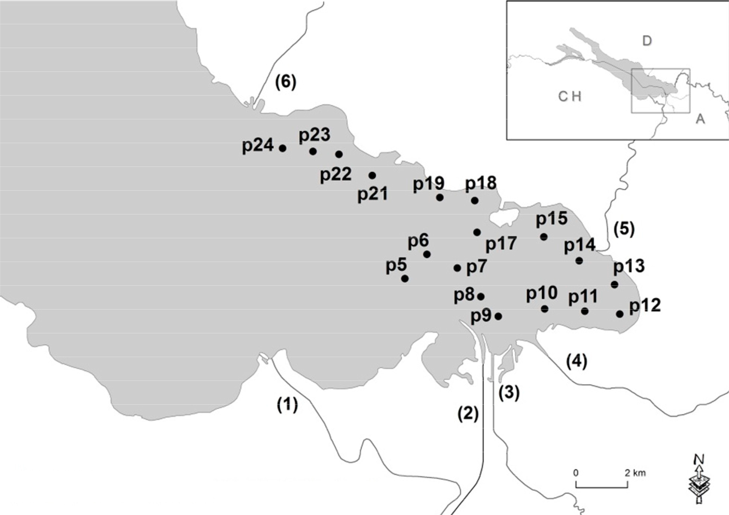
Lake Constance is located on the plateau north of the Alps, between Switzerland, Germany and Austria (Figure 1). The Alpine Rhine River (2, in Figure 1) discharges into the eastern basin, accounting for 62% of the total water input. The discharge reaches its maximum in late spring and early summer, due to massive snow melting. During this period, the river carries large loads of mineral particles [38], which create marked contrasts with the clear and oligotrophic lake water. Regarding the particle composition, Müller and Quakernaat [39] reported a dominance of the mica-chlorite assemblage near the Rhine inflow, and an increase of the smectite/mica ratio as moving westwards. In a more recent study, Schmieder et al. [40] analysed water samples near the shore, and confirmed the high variability of particle composition across the lake, in particular the “contribution of siliciclastic and dolomite minerals […] was much higher in the eastern parts of the lake than in the western parts”.
Other rivers may contribute to the lake’s IOPs only near their inflows. The Bregenzer Ach is another alpine river, and its waters are mineral-rich. In contrast, the catchment areas of the Leiblach and the Argen are plain lands of more intensive agricultural use, thus containing higher amounts of dissolved organic matter. Due to this complexity in the inflowing waters, the applicability of horizontally-invariant SIOPs needs to be tested.
2.2. Measured Data
The data presented in this paper was measured on 25 May 2012, collected at the sampling points shown in Figure 1. The samples were acquired between 9 am and 5 pm CEST.
A WET Labs C-star transmissometer measured light transmission profiles over a 10 cm optical path at 650 nm, from which the beam attenuation coefficient csm(650,z) (m−1) with respect to pure water was derived. csm(650,z) is expected to be linearly related to suspended matter [41], provided a background of low-to-medium CDOM absorption.
Gravimetric measurements were performed using Whatman GF/F filters, diameter 47 mm, pore size 0.7 µm, which were pre-heated at 450 °C for 100 min and then pre-weighted. Surface water samples (right below the surface to avoid floating particles) were taken, shaken and filtered. Afterwards, the filters were dried for 12 h at 50 °C and weighted again. The concentration sm(0−) was then calculated as the differential mass divided by the volume of filtered water.
Hemispherical-directional above-surface reflectance spectra were acquired using the Water Insight WISP-3 [42]. It is a hand-held spectrometer with three radiometers: one cosine receptor to measure the downwelling irradiance Ed(λ), and two Gershun tubes to measure the downwelling radiance from the sky Ld(λ, θ = 42°), and the total upwelling radiance Lu(λ, θ = 138°), θ being the polar angle, according to Mobley [43]. The measurement procedure was performed following Hommersom et al. [42]. Rrs(λ) was calculated as:
The original dataset consisted of 26 sampling points, from p0–p25 (Figure 1). However, Mobley [43] showed that for a viewing angle respect to nadir θv < 45°, the relationship ρ = 0.028 ceases to hold and ρ starts to increase with θv. By applying this constraint, we discarded p0–p04 and p25. To ensure the condition of optically-deep water, we discarded p16 and p20, which had a bottom depth zb < 7 m. The rest of the sampling points had zb > 25 m, with the sole exception of p17, with zb = 10 m but a very turbid sub-surface layer, so that bottom reflectance was unlikely.
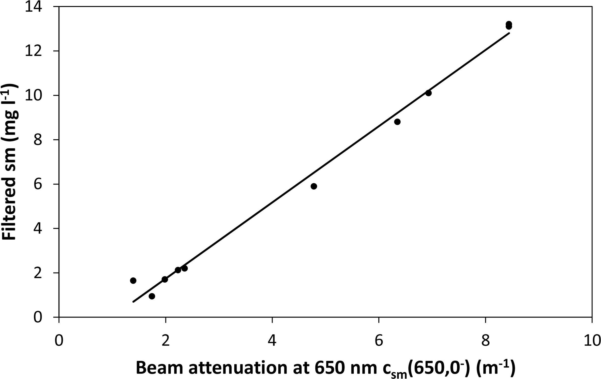
We constructed sm(z) using a linear regression between the particle beam attenuation at 650 nm just below the surface, csm(650,0−), and the concentration sm(0−) measured gravimetrically for the same sampling point. For this regression (Figure 2), we used only the sampling points that showed smooth near-surface profiles (for the GA procedure, all points were included instead). Then, we assumed that the particle composition of the surface samples can be extended to the first optical depth, so that the same SIOPs remain applicable. Under this assumption, we extended Equation (2) to the whole water column to construct the profiles sm(z):
The non-zero intercept in Equation (2) implies that light transmission for gravimetric sm = 0 is ∼90%. This issue is perhaps due to drift of the factory-supplied dark offset and does not affect the slope of Equation (2). A minor part of this background attenuation can be caused by particles smaller than 0.7 µm that are not retained on the filters.
The possible CDOM absorption at 650 nm is yet to be verified. Setting a spectral slope S = 0.014 nm−1 and a higher bound of CDOM absorption y(440) = 0.5 m−1 (higher values are unlikely in Lake Constance [5]) leads to y(650) = 0.264 m−1, which can be neglected for the magnitude range in Figure 2.
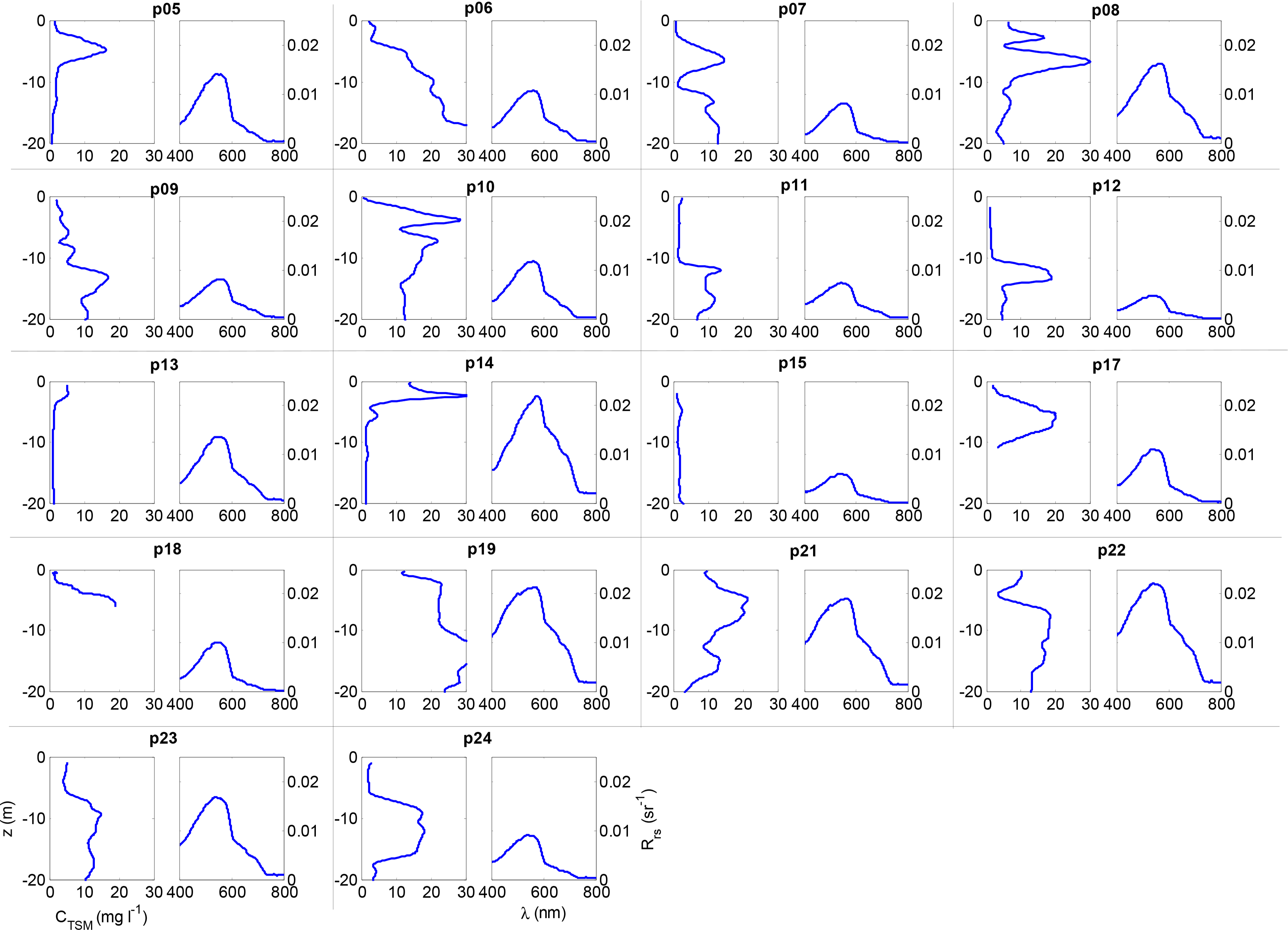
Figure 3 shows the measured Rrs(λ) and sm(z) for every sampling point. At first sight, sm(z) and Rrs(λ) seem to have a positive correlation. The profiles sm(z) always peak at a sub-surface layer, which in some cases is close to the surface. Therefore, it would be inappropriate to relate Rrs(λ) to surface values of sm. For instance, point p10 shows sm(0 m) < 1 mg·L−1 but a peak sm(4 m) ≈ 28 mg·L−1, whereas p11 shows a fairly constant sm ≈ 2.5 mg·L−1 from 0–10 m depth. As a result, Rrs(λ) is higher in p10 than in p11. The same happens between p05 and p06: p05 has a lower sm at the surface, but a higher Rrs(λ), due to a strong peak of sm(4.8 m) ≈ 16 mg·L−1, whereas for p06, sm(4.8 m) ≈ 12 mg·L−1.
The regression of Equation (2) can also be used as validation data for b*sm(λ) (derived in this article) at the wavelength 650 nm. We first assume absorption and scattering as proportional to the concentration, so we get:
We divide Equation (3) by sm(z) and apply Equation (2) after neglecting its residual term (attenuation by sm depends only on the linear term). We thereby quantify the mass-specific particle attenuation:
We assume a negligible a*sm(650) with respect to b*sm(650), which we justify as follows: non-algal absorption decays exponentially and can be estimated as negligible, or in the worst case, as a background value of 0.02 m2·g−1 (the existence of this background is controversial [44]). Mass-specific phytoplankton absorption at 650 nm has a value of ∼0.01 m2·g−1 [45], which finally leads to a total 0.03 m2·g−1. In contrast, b*sm(650) is never smaller than 0.3 m2·g−1 [44,46], which is 10 times more. Therefore, we obtain:
3. IOPs Modelling and Inversion
3.1. Optical Properties of Lake Constance
We model the IOPs of Lake Constance using a general case 2 scheme. Absorption a(λ,z) is separated into the following components: pure water (w), chl, and a single term for detritus, CDOM and mineral particles (dgm). Scattering b(λ,z) is assigned to water and particles. The spectral interval is between 400 and 800 nm. Table 1 includes all the variables used in the optical modelling.
Absorption of pure water is modelled using the measured spectra of Pope and Fry [47] and its scattering is computed using the formulas by Mobley [6].
Absorption by chl and its concentration are assumed to be linearly related [45,48]:
The choice of a*chl(λ) depends on the local phytoplankton species composition. This coefficient changes with space and time and is therefore a major source of uncertainty in spectral matching [49]. To partially overcome this problem, Gege [45] measured in-vitro a*chl(λ) of five typical phytoplankton classes in Lake Constance and proposed one average spectrum, which is used in this paper as in a previous study for Lake Constance [5]. We did not measure chl in our field work, so it is set as an unknown parameter.
For CDOM, a spectral exponential decay has been found appropriate [50]. Miksa et al. [51] measured in Lake Constance a decay constant S between 0.009 and 0.019 nm−1. The value S = 0.014 nm−1 was used to retrieve WQPs from MERIS data [5].
The spectral variation of the IOPs related to sm is less known. Detritus and mineral particle absorptions have been neglected in previous retrieval applications at Lake Constance [5,52], since significant contributions of the former are only expected for the Rhine delta region. From a large number of samples in coastal areas across Europe, Babin et al. [53] suggested that the absorption spectrum of detritus and mineral particles is well approximated by exponential decays, with a spectral decay close to 0.014 nm−1. The coincidence with the shape of CDOM makes the separation of detritus, CDOM and minerals from the bulk absorption an ill-posed problem, so we are forced to include them in a single exponentially-decaying term, with S = 0.014 nm−1:
Scattering by sm is widely modelled by a power law. Stramski et al. [46] found an exponent up to η = −1.3 for different types of particles in seawater. Odermatt et al. [5] used a power law for backscattering for remote sensing on Lake Constance, combined with a wavelength-independent bb,sm/bsm. The scattering magnitude at reference wavelengths varies between 0.5–1.5 m2·g−1 at 555 nm in Bowers and Binding [44] and 0.3–1.1 m2·g−1 at 400 nm in mineral-dominated assemblages by Woźniak et al. [12].
We model scattering by sm using the following product
Both b*sm(555) and η are left as unknown variables for optimization. The sm phase function is chosen from the Fournier-Forand family [54], using the ratio bb,sm/bsm = 0.019 [5,52]. This value is in agreement with measured values in water dominated by inorganic sediments [55].
3.2. Solving the Radiative Transfer Equation with Ecolight
Forward radiative transfer calculations are done using Ecolight, by Sequoia Scientific, Inc. [19]. Ecolight solves the azimuth-averaged RTE to obtain the radiance distribution as a function of depth, polar angle and wavelength. Ecolight is gaining popularity due to its good trade-off between speed and precision [16,56]. In this work, Ecolight is used instead of the more popular Hydrolight since the full angular radiance distribution is not needed, but only Rrs(λ). Our preliminary simulations showed a negligible difference in Rrs(λ) between Hydrolight and Ecolight, but at least 40 times faster performance for Ecolight. The source code of Ecolight has been compiled with the Intel Fortran Compiler 11.1 (IA-32) for Linux, included in the Intel® Composer XE 2013 compiling suite, and called from GNU Octave [57]. The input text files are automatically generated each run by ad-hoc Octave scripts.
Fluorescence by chl and CDOM, as well as Raman scattering are included in the simulation. The quantum yield of phytoplankton fluorescence is set to 0.02. CDOM fluorescence is not computed. The Raman scattering coefficient is set to 2.6 × 10⁻⁴ m−1 at the reference wavelength 488 nm and its corresponding phase function is set isotropic. The sun zenith angle is computed from time and location data. Normalized sky radiances are computed using the sky model of Harrison and Coombes [58], for an average cloud cover of 0.3. Diffuse and direct sky irradiances are computed using the RADTRANX model, included in the Ecolight software. The clear-sky irradiances are adjusted for cloudiness by the model of Kasten and Czeplak [59]. Other parameters are: atmospheric pressure 1012.53 hPa, air mass type 3, relative humidity 80%, precipitable water 2.5 cm, wind speed 4 m·s−1, visibility 15 km, ozone 330.1 Dobson units and an aerosol optical thickness of 0.261 at 550 nm. The index of refraction of water is calculated for an average water temperature of 14 °C and negligible salinity. The parameters mentioned in this paragraph are left constant for all sampling points, which were sampled within a few hours. Finally, the water column is considered infinitely deep.
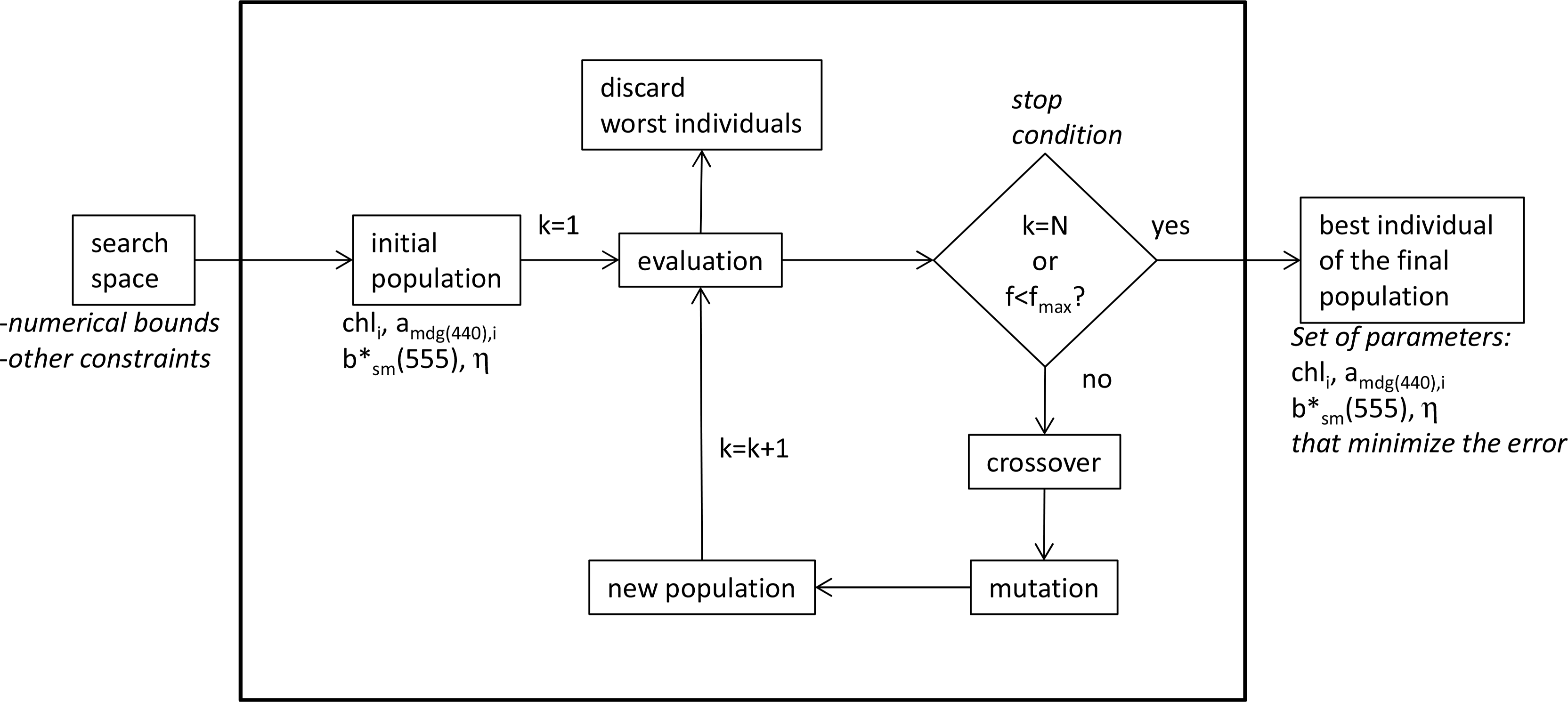
3.3. Inverting the Radiative Transfer Equation with Genetic Algorithms
The goal of the optimization procedure (Figure 4) is to retrieve the unknown variables of Table 1 by spectral matching of Rrs(λ). The goal function f in Equation (11) is built consequently, as the relative RMS error across the spectrum, and posteriorly averaged across sampling points. Nλ is the number of spectral bands and Np is the number of sampling points. The error is chosen as relative instead of absolute to give the same importance to all the sampling points, which have largely different peak values of Rrs(λ).
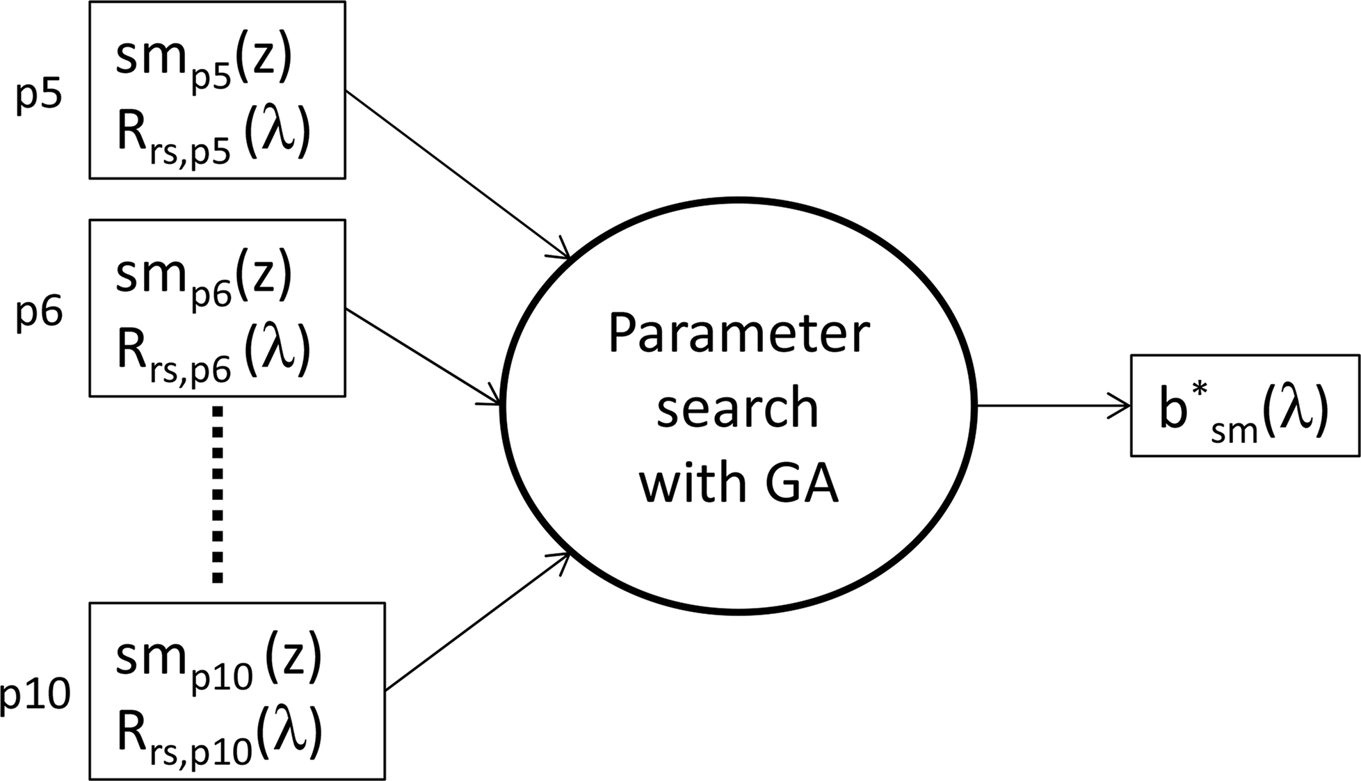
We arbitrarily choose six first valid points (p05–p10, Figure 1) to derive b*sm(λ). The optical model is forced at each point with the corresponding sm(z). The parameter search finds the b*sm(λ) leading to the best fitness, as defined in Equation (11). A general scheme of this GA procedure is shown in Figure 5. The mass-specific scattering coefficient b*sm(λ) is expected to have much less spatial variability than any IOP, as far as the particle composition remain constant at the given lake area. On the other hand, adgm(λ) depends on the actual concentrations of CDOM and sm, thereby its value needs to be determined individually at each point.
For the spectral range, we use 16 spectral bands for simulation in Ecolight, from 400–800 nm with 25 nm bandwidth, covering the full range measured by the WISP-3. The measured Rrs(λ) are interpolated to the same grid for comparison.
We use the GA software package developed by Houck et al. [60] under the GNU General Public License. Figure 4 illustrates the flow chart of a GA routine. The working principle mimics the evolutionary “survival of the fittest” [61]. Every unknown variable (every row of the column “Parameter” of Table 2) is called a gene, and the vector formed with a set of genes is called an individual. One individual is a complete set of model parameters that provide one model result (in our case, one set of bio-physical parameters that determine a single solution of the RTE). GA are initialized with an initial random population of individuals (first generation, k = 1), taken from a search space, which is the set of all possible values of the individuals, based on numerical bounds and other constraints. The bounds are specified in Table 2, column “Range”. No further constraints are set. The goal function f is evaluated by calling the bio-physical model (in our case, the solution of the RTE) for all individuals. The individuals that perform worst in terms of the goal function (in our case, the highest deviation from the observations) are eliminated and the rest are exposed to crossover, in which couples are formed and their genes exchanged, giving each birth to a pair of children. A subset of the offspring is exposed to a mutation process, in which several genes from certain individuals undergo a change in their values. The offspring forms the next generation (k → k + 1) and the process is repeated. The set-up of the GA parameters are left as the default values in Houck et al. [60]. The process is repeated until the maximum number of generations is achieved (k = N) or the goal function meets the requirements (f < fmax). The random component of GA lies in the crossover and mutation. On the other hand, the selection is deterministic. For detailed explanations, with focus on practical applications, the reader is referred to Haupt and Haupt [62].
Due to the random component of the GA, different optimizations do not necessarily lead to the same results, despite having the same initial search space. In a multidimensional space, a sufficient number of individuals must be spread, and for a given population density, the number of individuals grows exponentially with the number of dimensions. In our case (14 dimensions, see Table 2), the number of individuals should be high, but this is limited by computing and memory resources. We iteratively increased the population of the GA and found sufficient convergence when 200 individuals are chosen. The number of generations was set to 60. This lead to 12,000 evaluations of the bio-optical model.
3.4. Vertical Averaging of the Suspended Matter Profiles
Remote sensing algorithms retrieve sm concentrations that compare to a vertically-weighted average of the in-situ measured sm profiles, according to light extinction. To average our in-situ data, we use the following weighting function, which includes the round trip attenuation to depth z according to the diffuse attenuation coefficients of upwelling and downwelling irradiances (Kd and Ku) [63]:
Ecolight provides inaccurate Kd and Ku if the output depths are not closely spaced. Instead, Hydrolight adds automatically new depths close to the output depths to provide accurate values. We therefore obtain Kd and Ku by Hydrolight simulations of each sampling point, using the same input data as for Ecolight.
The weighting function of Equation (12) is wavelength-dependent. To obtain a single depth-averaged sm, we need to perform a wavelength average,
3.5. Comparison to the Quasi-Analytical Algorithm
The QAA (version 5) [37] is a semi-analytical algorithm that combines analytical IOP modelling with empirical coefficients. It was calibrated using data of oceanic and coastal waters and introduces several changes with respect to former versions. Contrary to analytical algorithms, the QAA does not require optical closure for the full spectrum and therefore does not make use of any assumed SIOP. For further details, the reader is referred to Lee et al. [37].
Spectral backscattering is modelled through a power law:
The reference value at 555 nm bb,sm(555) and the exponent η have been estimated from Rrs(λ).
For sm, QAA’s output value is bb,sm(555). To relate backscattering to the actual concentration, a given mass-specific backscattering (external to the QAA procedure) is needed as ancillary knowledge. Here, we use our assumed back-scattering to scattering ratio bb,sm/bsm = 0.019 and the reference value b*sm(650) = 0.6 m2·g−1 in order to get:
4. Results and Discussion
4.1. Derivation of the Mass-Specific Suspended Matter Scattering Coefficient
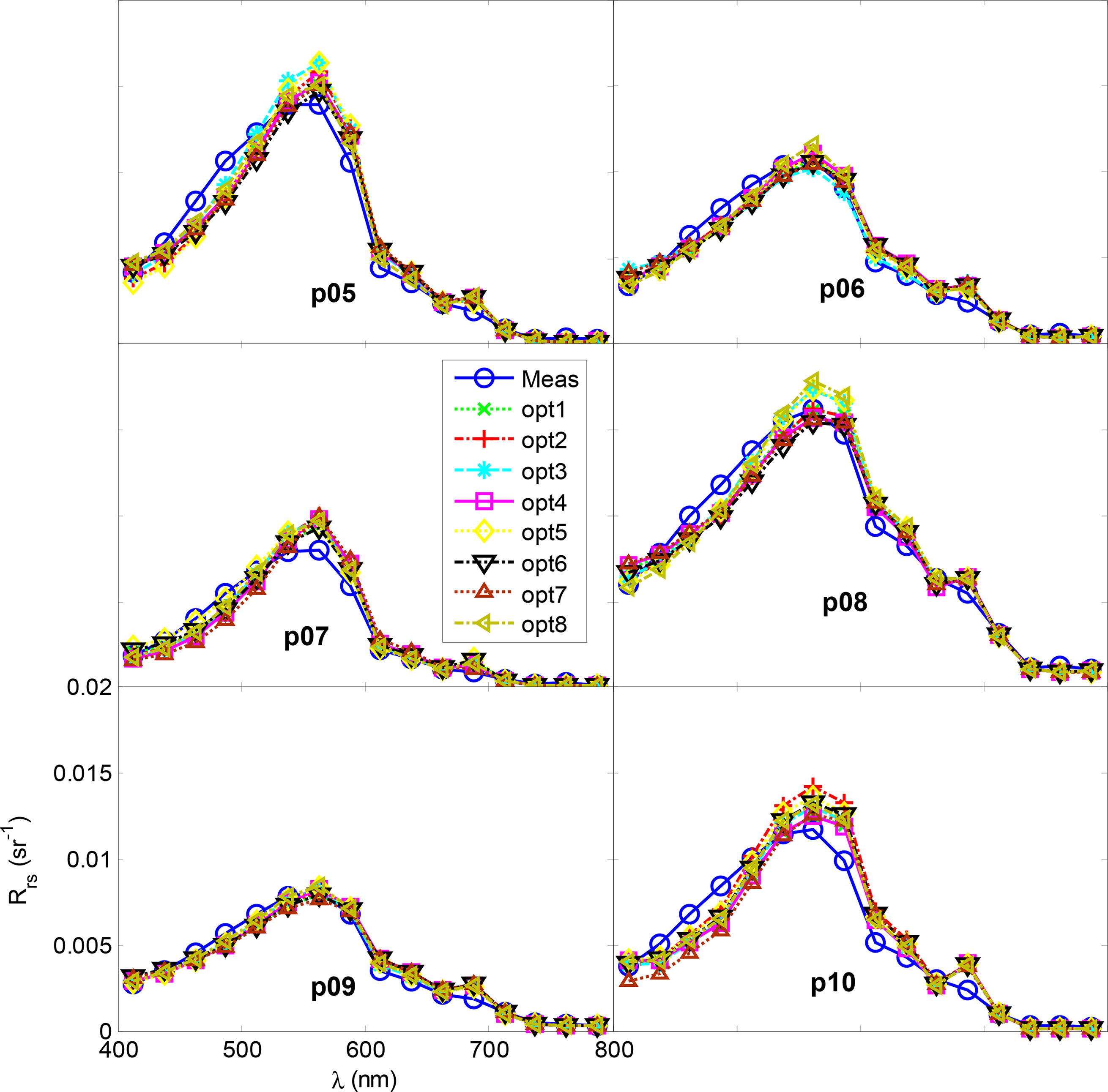
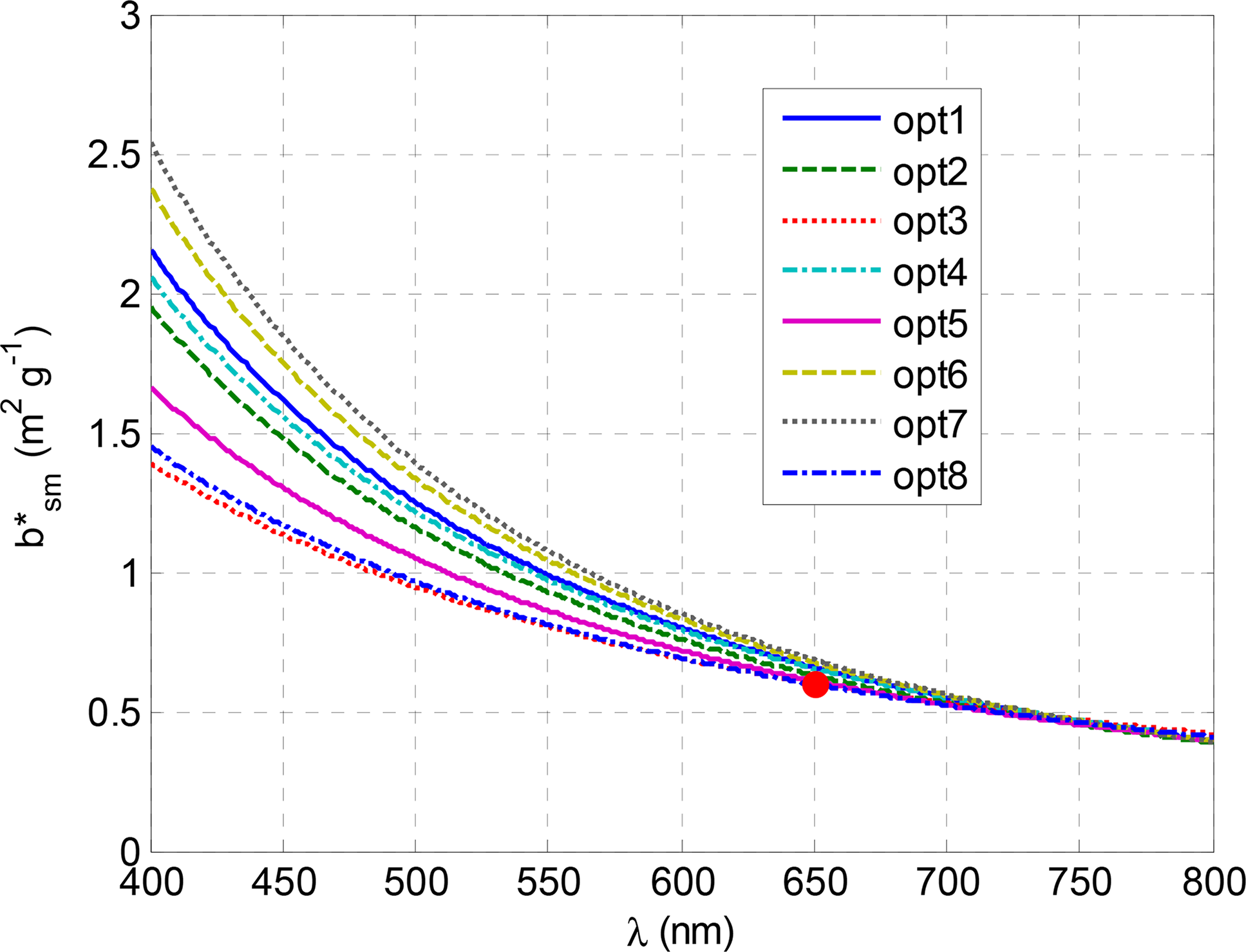
We performed eight independent optimizations with the same range of parameter search (Table 2). As GA have random components (initial solution and mutation), results may vary among optimizations. Figure 6 shows the matched Rrs(λ) for each point and each optimization. All the optimizations achieved a good degree of agreement (f < 5.1%). Table 2 below summarizes the different solutions. b*sm(555) shows values between 0.80 and 1.02 m2·g−1, and the exponent η varies between −2.70 and −1.73. Figure 7 depicts the reconstructed spectral b*sm(λ) for each optimization. The relatively steep slope η for all cases suggests a predominance of small particles in the size distribution, which could also explain the residual scattering found in Equation (2). Differences among curves at blue wavelengths indicate that adgm(λ), achl(λ) and bsm(λ) are affected by spectral ambiguity, due to similar spectral shapes [64]. On the contrary, ambiguity is minor at green to red wavelengths, because adgm(λ) vanishes and because the shapes of achl(λ) and bsm(λ) are very different at that region of the spectrum. Therefore, all the optimizations show very similar b*sm(λ), approaching b*sm(650) ≈ 0.6 m2·g−1, in agreement with the value derived from the transmissometer measurements in Equations (2)–(5) (red dot in Figure 7).
In order to decide which optimization to choose as best result, we apply a posteriori physical constraints: Values b*sm(400) > 1.5 m2·g−1 are very unlikely [46], so we select only optimizations resulting in b*sm(400) < 1.5 m2·g−1 (opt3 and opt8 in Table 2). Additionally, they show the best Rrs(λ) match. opt8 has a slightly lower error, so we finally choose it as the best solution. Figure 8 shows b*sm(λ) = 0.80(λ/555)−1.82 (opt8) together with previously published data.
Afterwards, we performed several optimizations in which we replaced the constrain b*(555) ∈ [0.1, 1.5] m2·g−1 with b*(400) ∈ [0.1, 1.5] m2·g−1. For a typical spectral shape of b*, this constrain is more restrictive, as b* tends to increase towards the blue. We find b*(400) ranging from 0.75–1.2 m2·g−1 and η ranging from −0.8 to −1.6. Again, b*(400) and η combine in a fashion leading to b*(650) close to 0.6 m2·g−1, as already depicted in Figure 7 (the most distant, 0.52 m2·g−1). Thus, the range of ambiguity in b*(400) extends towards lower (and probably, more physical) values than those depicted in Figure 7, but always tending to uniqueness towards the red. Therefore, it is more illustrative to present the specific scattering with a reference wavelength of 650 nm instead of 555 nm, so that the reference value is quite certain, while all the uncertainty is contained in the exponent. The final expression is then: b*sm(λ) = 0.60(λ/650)−1.82.
Although the goal of this paper is to retrieve b*sm(λ), we make some comments on the other quantities. The chl and adgm(λ) retrievals are affected by the spectral ambiguity previously commented. They are too high for all but opt3 and opt8 (adgm up to 0.93 m−1, chl up to 19 µg·L−1). For opt3 and 8 they show more realistic values but are probably still too high [65] (pp. 46–47).
Figure 6 shows that p10 yields the worst spectral fitness of all, probably due to a higher degree of measurement uncertainty. In fact, p10 shows the most unrealistic chl values. However, as the goal function f in Equation (11) is an average of six points, a higher error in one of them is accepted, yet keeping f low. It is worth noting that, although the spectral shape of adgm(λ) is accepted to be exponential, the achl(λ) used in this article [45] can have significant deviations from the real value.
4.2. Validation
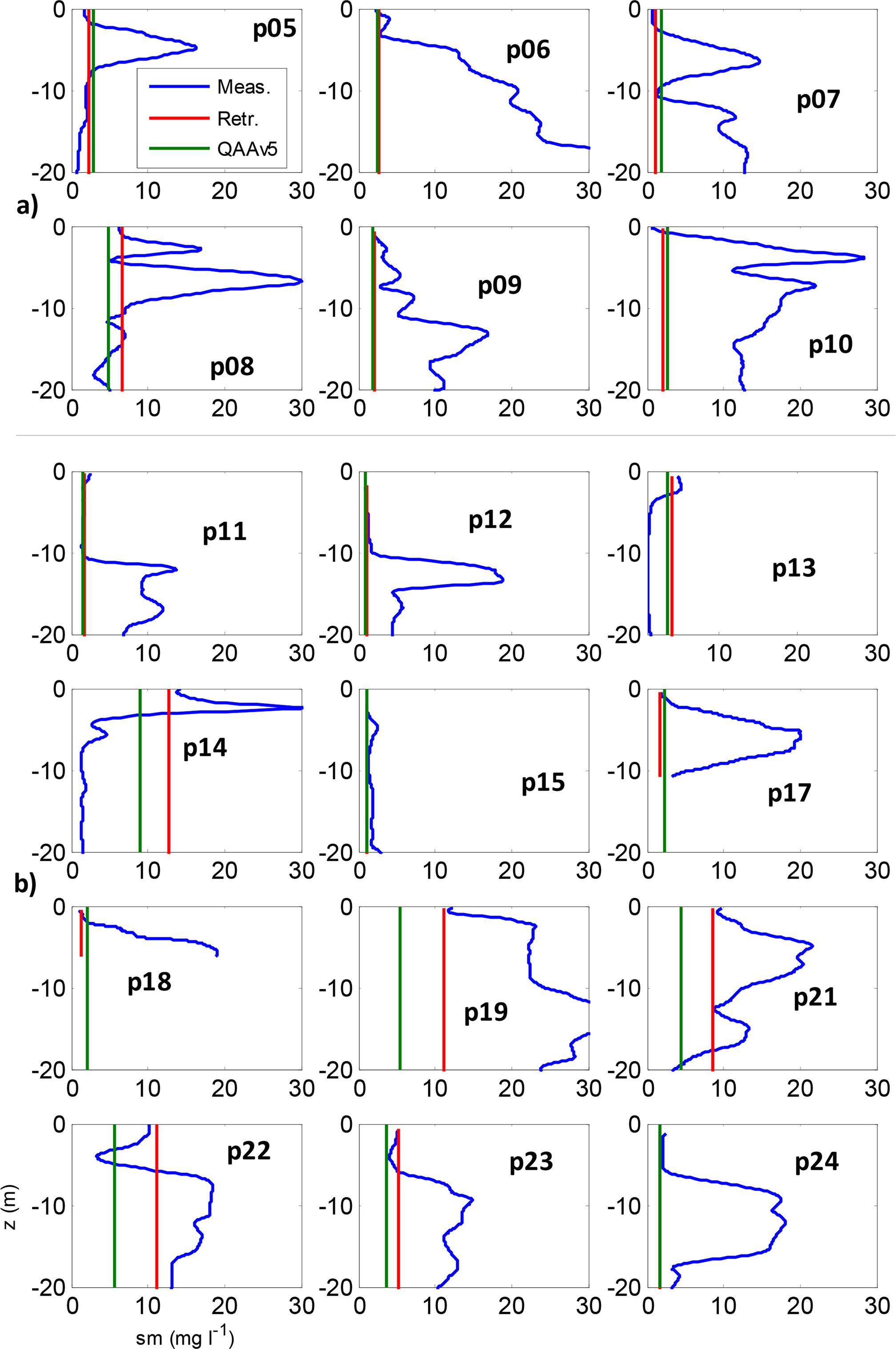
In the previous section, we derived b*sm(λ) = 0.60(λ/650)−1.82 (opt 8 in Table 2) using the sm concentrations of p05–p10. Now, as validation, we leave b*sm(λ) fixed as ancillary knowledge and retrieve the apparent, vertically constant sm profiles (smret) for comparison with the in-situ measured sm(z). The retrieval is made separately for each sampling point by spectral matchup of Rrs(λ) with points p050–p10 (calibration dataset) and p11–p24 (independent dataset). We performed a single sm retrieval (for every single sampling point) in Section 4.2 because we found very satisfactory results (shown in Figure 9). Posterior repeated runs (results not shown) for each point revealed a remarkable robustness of the retrievals for the high sm values (sm > 3 mg·L−1). However, for the clearest waters, the retrieval is affected by some uncertainty. It seems that, when sm dominates the optical properties (wavelength-averaged in our approach), the solution of the inverse problem tends to uniqueness. The reader should also note that the good correlation coefficient is mainly driven by the high sm values (Figure 10). This outcome is of no surprise, since it would be difficult to have such good retrieval by coincidence.
Figure 9 shows the superimposed measured sm(z) (blue) and smret (red) for every point. For all points, the match between smret and the measured sm(z) seems excellent for the upper layer, even for the independent dataset, which was not used to derive b*sm(λ).
Application of the QAA to our dataset yields values for η ranging from −0.26 at p07 to −0.75 at p19, which are much flatter than our retrieved η = −1.82. By defining b*sm,QAA(650) = 0.6 m2·g−1 and applying the QAA spectral slopes at each point, all the point-specific b*sm,QAA(λ) are plotted in Figure 8. Retrievals of sm by the QAA are calculated using Equation (15) and shown in green in Figure 9. The QAA seems to underestimate high sm values.
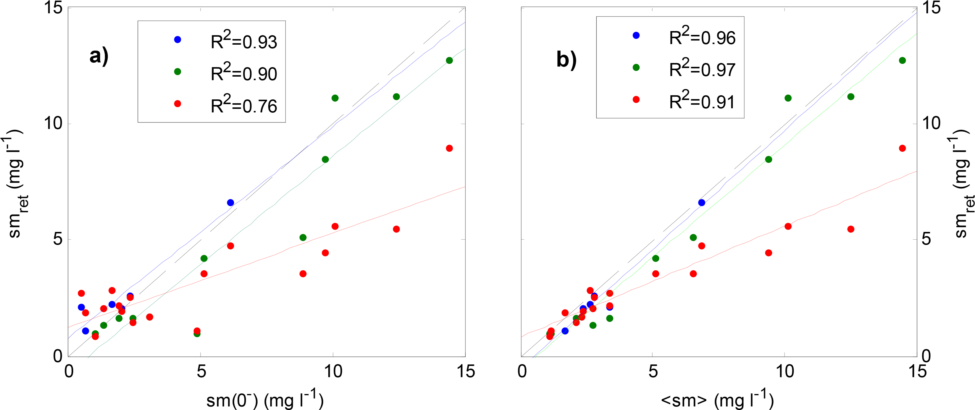
To perform a numerical comparison among profiles in Figure 9, the measured sm(z) are vertically averaged using Equation (12). The regression analysis performed in Figure 10 between <sm> and smret shows the quality of the sm retrievals using our algorithm for the calibration dataset (p5–p10) in blue, using our algorithm for the validation dataset (p11–p24) in green, and using the QAA for all points (in red). The left graph (a) compares the retrievals with respect to a single sub-surface measured value, sm(0−), whereas the right graph (b) compares with respect to the vertically-averaged measured value, <sm> (Equation (12)). These results highlight the following:
- (1)
R2 improves if we consider the entire profile to evaluate the retrieval ((b) in Figure 10) than if we only consider a sub-surface measured value ((a) in Figure 10). The reason is due to the strong vertical variability of sm(z) (blue in Figure 10, in particular, p3, p4, p5, p8, p13, p19 and p20). In these cases, a single depth is not representative for the sake of algorithm development and evaluation, but the whole profile is needed due to light penetration [15,16,18].
- (2)
R2 does not significantly decrease for the validation dataset (green in Figure 10) compared to the calibration dataset (blue in Figure 10), in spite of the expected ambiguity of our b*sm(λ) estimate and the absorption variables in the bio-optical model. We can thus conclude that the expected ambiguity does not lead to retrieval failure as far as our limited dataset is concerned.
- (3)
The QAA underestimates <sm> by a factor of 1/0.577 when using the derived b*sm(650) = 0.6 m2·g−1 and the assumed bb,sm/bsm = 0.019 in Equation (15). To compensate for this factor, we could keep bb,sm/bsm = 0.019 and set b*sm,QAA(650) = 0.6·0.577 m2·g−1 = 0.346 m2·g−1. This value is in the lower range of published data (Figure 8) and differs from b*sm(650) = 0.6 m2·g−1, which we derived independently. On the other hand, if we keep b*sm,QAA(650) = 0.6 m2·g−1, we get bb,sm/bsm = 0.011, unlikely for mineral-dominated suspended matter [55]. The discrepancy seems to rely on the QAA retrieval of backscattering. Given the good correlation R2 = 0.91 to in situ data, it seems that, after a custom QAA calibration, the best fit could be brought to the 1:1 line. Nonetheless, this latter task is beyond the scope of this article.
5. Conclusions
In this paper, we achieved radiative transfer closure between IOPs and Rrs(λ) using Ecolight for Radiative Transfer modelling and genetic algorithms (GA) for parameter search. Using a subset of our field data, we retrieved a b*sm(λ) consistent with independent measurements at 650 nm. This b*sm(λ) was used as ancillary data to perform a remote sensing retrieval of suspended matter smret, comparing very well to in-situ independent data (R2 > 0.95). The robustness in the sm retrievals is somehow surprising given the insufficient constraint of the bio-optical model with our available measurements. Further evaluation of the algorithm will aim at a validation with accurate SIOP measurements. This will allow assessing different additional constraints, and making a direct comparison of measured and retrieved b*sm(λ).
Acknowledgments
The research leading to these results has received funding from the European Union Seventh Framework Programme (FP7/2007–2013) under grant agreement n° 263287 (FRESHMON project). The field work was part of validation activities of satellite-retrieved suspended matter in Lake Constance. Many thanks go to our colleagues Michael Schurter, Alois Zwyssig and Brandon Hicks (technicians) and Elisabeth Eder (PhD student) for their support during field work, and to Rosi Siber (GIS expert) for the figure of Lake Constance. We thank Roland Riederer and Silvio Müller from the Administration of Kanton Sankt Gallen, as well as Hildegard Bischof, from Hafen am Rheinspitz, for providing a parking place for the boat. We are also grateful to our project partners Thomas Heege and Karin Schenk, of EOMAP, for managing the project and to Water Insight, for providing the WISP. Devis Tuia and Isabel Kiefer, from EPFL, are acknowledged for their comments and Lee D Bryant for linguistic advice. Finally, we thank three anonymous reviewers for their constructive comments.
Author Contributions
All authors conceived and designed the experiment; Jaime Pitarch, Daniel Odermatt and Marcin Kawka performed the experiment; Jaime Pitarch analyzed the data and designed the model supported by Daniel Odermatt; Jaime Pitarch wrote the article with contributions and corrections by Daniel Odermatt, Marcin Kawka and Alfred Wüest.
Conflicts of Interest
The authors declare no conflict of interest.
References
- Bresciani, M.; Stroppiana, D.; Odermatt, D.; Morabito, G.; Giardino, C. Assessing remotely sensed chlorophyll-a for the implementation of the Water Framework Directive in European perialpine lakes. Sci. Total Environ 2011, 409, 3083–3091. [Google Scholar]
- Chen, Q.; Zhang, Y.; Ekroos, A.; Hallikainen, M. The role of remote sensing technology in the EU Water Framework Directive (WFD). Environ. Sci. Policy 2004, 7, 267–276. [Google Scholar]
- Domínguez, J.A.; Alonso, C.; Alonso, A. Remote sensing as a tool for monitoring water quality parameters for Mediterranean lakes of European Union Water Framework Directive (WFD) and as a system of surveillance of cyanobacterial harmful algae blooms (SCyanoHABs). Environ. Monit. Assess 2011, 181, 317–334. [Google Scholar]
- Hadjimitsis, D.; Clayton, C. Assessment of temporal variations of water quality in inland water bodies using atmospheric corrected satellite remotely sensed image data. Environ. Monit. Assess 2009, 159, 281–292. [Google Scholar]
- Odermatt, D.; Heege, T.; Nieke, J.; Kneubühler, M.; Itten, K. Water quality monitoring for Lake Constance with a physically based algorithm for MERIS data. Sensors 2008, 8, 4582–4599. [Google Scholar]
- Mobley, C.D. Light and Water: Radiative Transfer in Natural Waters; Academic Press: San Diego, CA, USA, 1994; Volume 592. [Google Scholar]
- Prieur, L.; Sathyendranath, S. An optical classification of coastal and oceanic waters based on the specific spectral absorption curves of phytoplankton pigments, dissolved organic matter, and other particulate materials. Limnol. Oceanogr 1981, 26, 671–689. [Google Scholar]
- Roesler, C.S.; Perry, M.J.; Carder, K.L. Modeling in situ phytoplankton absorption from total absorption spectra in productive inland marine waters. Limnol. Oceanogr 1989, 34, 1510–1523. [Google Scholar]
- Bricaud, A.; Babin, M.; Morel, A.; Claustre, H. Variability in the chlorophyll-specific absorption coefficients of natural phytoplankton: Analysis and parameterization. J. Geophys. Res. Oceans 1995, 100, 13321–13332. [Google Scholar]
- Bricaud, A.; Babin, M.; Claustre, H.; Ras, J.; Tièche, F. Light absorption properties and absorption budget of Southeast Pacific waters. J. Geophys. Res. Oceans 2010, 115, C08009. [Google Scholar]
- Babin, M.; Morel, A.; Fournier-Sicre, V.; Fell, F.; Stramski, D. Light scattering properties of marine particles in coastal and open ocean waters as related to the particle mass concentration. Limnol. Oceanogr 2003, 48, 843–859. [Google Scholar]
- Woźniak, S.B.; Stramski, D.; Stramska, M.; Reynolds, R.A.; Wright, V.M.; Miksic, E.Y.; Cichocka, M.; Cieplak, A.M. Optical variability of seawater in relation to particle concentration, composition, and size distribution in the nearshore marine environment at Imperial Beach, California. J. Geophys. Res. Oceans 2010, 115, C08027. [Google Scholar]
- Matsuoka, A.; Hill, V.; Huot, Y.; Babin, M.; Bricaud, A. Seasonal variability in the light absorption properties of western Arctic waters: Parameterization of the individual components of absorption for ocean color applications. J. Geophys. Res. Oceans 2011, 116, C02007. [Google Scholar]
- Gordon, H.R. Simple calculation of the diffuse reflectance of the ocean. Appl. Opt 1973, 12, 2803–2804. [Google Scholar]
- Stramska, M.; Stramski, D. Effects of a nonuniform vertical profile of chlorophyll concentration on remote-sensing reflectance of the ocean. Appl. Opt 2005, 44, 1735–1747. [Google Scholar]
- Yang, Q.; Stramski, D.; He, M.-X. Modeling the effects of near-surface plumes of suspended particulate matter on remote-sensing reflectance of coastal waters. Appl. Opt 2013, 52, 359–374. [Google Scholar]
- Effler, S.W.; Matthews, D.A.; Kaser, J.W.; Prestigiacomo, A.R.; Smith, D.G. Runoff event impacts on a water supply reservoir: Suspended sediment loading, turbid plume behavior, and sediment deposition. J. Am. Water Resour. Assoc 2006, 42, 1697–1710. [Google Scholar]
- Bélanger, S.; Cizmeli, S.A.; Ehn, J.; Matsuoka, A.; Doxaran, D.; Hooker, S.; Babin, M. Light absorption and partitioning in Arctic Ocean surface waters: Impact of multiyear ice melting. Biogeosciences 2013, 10, 6433–6452. [Google Scholar]
- Mobley, C.D.; Sundman, L.K. Hydrolight 5 Technical Documentation. Available online: http://www.hydrolight.info (accessed on 10 January 2012).
- IOCCG, Remote Sensing of Inherent Optical Properties: Fundamentals, Tests of Algorithms and Applications; International Ocean Colour Coordinating Group (IOCCG): Dartmouth, NS, Canada, 2006; p. 126.
- Davis, L. Handbook of Genetic Algorithms; Van Nostrand Reinhold: New York, NY, USA, 1991. [Google Scholar]
- Michalewicz, Z. Genetic Algorithms + Data Structures = Evolution Programs; Springer Verlag: Berlin/Heidelberg, Germany, 1994; p. 387. [Google Scholar]
- Renner, G.; Ekárt, A. Genetic algorithms in computer aided design. Comput. Aided Des 2003, 35, 709–726. [Google Scholar]
- Wang, Q.J. Using genetic algorithms to optimise model parameters. Environ. Model. Softw 1997, 12, 27–34. [Google Scholar]
- Tseng, M.-H.; Chen, S.-J.; Hwang, G.-H.; Shen, M.-Y. A genetic algorithm rule-based approach for land-cover classification. ISPRS J. Photogramm. Remote Sens 2008, 63, 202–212. [Google Scholar]
- Liu, Z.; Liu, A.; Wang, C.; Niu, Z. Evolving neural network using real coded genetic algorithm (GA) for multispectral image classification. Future Gener. Comput. Syst 2004, 20, 1119–1129. [Google Scholar]
- Bandyopadhyay, S.; Pal, S.K. Pixel classification using variable string genetic algorithms with chromosome differentiation. IEEE Trans. Geosci. Remote Sens 2001, 39, 303–308. [Google Scholar]
- Fang, H.; Liang, S.; Kuusk, A. Retrieving leaf area index using a genetic algorithm with a canopy radiative transfer model. Remote Sens. Environ 2003, 85, 257–270. [Google Scholar]
- Li, L.; Cheng, Y.B.; Ustin, S.; Hu, X.T.; Riaño, D. Retrieval of vegetation equivalent water thickness from reflectance using genetic algorithm (GA)-partial least squares (PLS) regression. Adv. Space Res 2008, 41, 1755–1763. [Google Scholar]
- Hansen, M.C.; DeFries, R.S.; Townshend, J.R.G.; Carroll, M.; Dimiceli, C.; Sohlberg, R.A. Global percent tree cover at a spatial resolution of 500 meters: First results of the MODIS vegetation continuous fields algorithm. Earth Interact 2003, 7, 1–15. [Google Scholar]
- Chami, M.; Robilliard, D. Inversion of oceanic constituents in case I and II waters with genetic programming algorithms. Appl. Opt 2002, 41, 6260–6275. [Google Scholar]
- Zhang, H.; Lee, Z.-P.; Shi, P.; Chen, C.; Carder, K.L. Retrieval of water optical properties for optically deep waters using genetic algorithms. IEEE Trans. Geosci. Remote Sens 2003, 41, 1123–1128. [Google Scholar]
- Chang, C.H.; Liu, C.-C.; Wen, C.G. Integrating semianalytical and genetic algorithms to retrieve the constituents of water bodies from remote sensing of ocean color. Opt. Express 2007, 15, 252–265. [Google Scholar]
- Chen, L.; Tan, C.-H.; Kao, S.-J.; Wang, T.-S. Improvement of remote monitoring on water quality in a subtropical reservoir by incorporating grammatical evolution with parallel genetic algorithms into satellite imagery. Water Res 2008, 42, 296–306. [Google Scholar]
- Huang, C.-C.; Li, Y.-M.; Sun, D.-Y.; Le, C.-F. Retrieval of Microcystis aentginosa percentage from high turbid and eutrophia inland water: A case study in Taihu Lake. IEEE Trans. Geosci. Remote Sens 2011, 49, 4090–4100. [Google Scholar]
- Song, K.; Lu, D.; Li, L.; Li, S.; Wang, Z.; Du, J. Remote sensing of chlorophyll-a concentration for drinking water source using genetic algorithms (GA)-partial least square (PLS) modeling. Ecol. Inform 2012, 10, 25–36. [Google Scholar]
- Lee, Z.P.; Lubac, B.; Werdell, J.; Arnone, R. An Update of the Quasi-Analytical Algorithm (QAA_v5). Available online: http://www.ioccg.org/groups/Software_OCA/QAA_v5.pdf (accessed on 11 August 2013).
- Fuentes, N.; Güde, H.; Wessels, M.; Straile, D. Allochthonous contribution to seasonal and spatial variability of organic matter sedimentation in a deep oligotrophic lake (Lake Constance). Limnologica 2013, 43, 122–130. [Google Scholar]
- Müller, G.; Quakernaat, J. Diffractometric clay mineral analysis of recent sediments of Lake Constance (Central Europe). Contrib. Mineral. Petrol 1969, 22, 268–275. [Google Scholar]
- Schmieder, K.; Schünemann, B.; Schröder, H.G. Spatial patterns of surface sediment variables in the littoral zone of Lake Constance (Germany). Arch. Hydrobiol 2004, 161, 455–468. [Google Scholar]
- Guillén, J.; Palanques, A.; Puig, P.; Durrieu de Madron, X.; Nyffeler, F. Field calibration of optical sensors for measuring suspended sediment concentration in the western Mediterranean. Sci. Mar 2000, 64, 427–435. [Google Scholar]
- Hommersom, A.; Kratzer, S.; Laanen, M.; Ansko, I.; Ligi, M.; Bresciani, M.; Giardino, C.; Beltrán-Abaunza, J.M.; Moore, G.; Wernand, M.; et al. Intercomparison in the field between the new WISP-3 and other radiometers (TriOS Ramses, ASD FieldSpec, and TACCS). J. Appl. Remote Sens 2012, 6. [Google Scholar] [CrossRef]
- Mobley, C.D. Estimation of the remote-sensing reflectance from above-surface measurements. Appl. Opt 1999, 38, 7442–7455. [Google Scholar]
- Bowers, D.G.; Binding, C.E. The optical properties of mineral suspended particles: A review and synthesis. Estuar. Coast. Shelf Sci 2006, 67, 219–230. [Google Scholar]
- Gege, P. Characterization of the phytoplankton in Lake Constance for classification by remote sensing (with 6 figures and 2 tables). In Lake Constance, Characterization of an Ecosystem in Transition; Baeuerle, E., Gaedke, U., Eds.; E. Schweizerbart’sche Verlagsbuchhandlung (Nägele und Obermiller): Stuttgart, Germany, 1998; pp. 179–194. [Google Scholar]
- Stramski, D.; Babin, M.; Wozniak, S.B. Variations in the optical properties of terrigenous mineral-rich particulate matter suspended in seawater. Limnol. Oceanogr 2007, 52, 2418–2433. [Google Scholar]
- Pope, R.M.; Fry, E.S. Absorption spectrum (380–700 nm) of pure water. II. Integrating cavity measurements. Appl. Opt 1997, 36, 8710–8723. [Google Scholar]
- Albert, A.; Mobley, C. An analytical model for subsurface irradiance and remote sensing reflectance in deep and shallow case-2 waters. Opt. Express 2003, 11, 2873–2890. [Google Scholar]
- Kostadinov, T.S.; Siegel, D.A.; Maritorena, S.; Guillocheau, N. Ocean color observations and modeling for an optically complex site: Santa Barbara Channel, California, USA. J. Geophys. Res. Oceans 2007, 112, C07011. [Google Scholar]
- Bricaud, A.; Morel, A.; Prieur, L. Absorption by dissolved organic matter of the sea (yellow substance) in the UV and visible domains. Limnol. Oceanogr 1981, 26, 43–53. [Google Scholar]
- Miksa, S.; Gege, P.; Heege, T. Investigations on the capability of CHRIS-Proba for monitoring of water constituents in Lake Constance compared to MERIS. In Proceedings of the 2nd CHRIS-PROBA Workshop, Frascati, Italy, 28–30 April 2004.
- Heege, T. Flugzeuggestützte Fernerkundung von Wasserinhaltsstoffen im Bodensee. Ph.D. Dissertation, Deutsches Zentrum für Luft- und Raumfahrt, Köln, Germany. 2000, 134. [Google Scholar]
- Babin, M.; Stramski, D.; Ferrari, G.M.; Claustre, H.; Bricaud, A.; Obolensky, G.; Hoepffner, N. Variations in the light absorption coefficients of phytoplankton, nonalgal particles, and dissolved organic matter in coastal waters around Europe. J. Geophys. Res. Oceans 2003, 108. [Google Scholar] [CrossRef]
- Mobley, C.D.; Sundman, L.K.; Boss, E.L. Phase function effects on oceanic light fields. Appl. Opt 2002, 41, 1035–1050. [Google Scholar]
- Boss, E.; Pegau, W.S.; Lee, M.; Twardowski, M.; Shybanov, E.; Korotaev, G.; Baratange, F. Particulate backscattering ratio at LEO 15 and its use to study particle composition and distribution. J. Geophys. Res. Oceans 2004, 109, C01014. [Google Scholar]
- Saulquin, B.; Hamdi, A.; Gohin, F.; Populus, J.; Mangin, A.; d’Andon, O.F. Estimation of the diffuse attenuation coefficient KdPAR using MERIS and application to seabed habitat mapping. Remote Sens. Environ 2013, 128, 224–233. [Google Scholar]
- Eaton, J.W.; Bateman, D.; Hauberg, S. GNU Octave. A High-Level Interactive Language for Numerical Computations; Free Software Foundation, Inc.: Boston, MA, USA, 2011; p. 812. [Google Scholar]
- Harrison, A.W.; Coombes, C.A. An opaque cloud cover model of sky short wavelength radiance. Sol. Energy 1988, 41, 387–392. [Google Scholar]
- Kasten, F.; Czeplak, G. Solar and terrestrial radiation dependent on the amount and type of cloud. Sol. Energy 1980, 24, 177–189. [Google Scholar]
- Houck, C.R.; Joines, J.A.; Kay, M.G. A Genetic Algorithm for Function Optimization: A Matlab Implementation; NCSU-IE-TR-95-09; North Carolina State University: Raleigh, NC, USA, 1995. [Google Scholar]
- Chaturvedi, D.K. Genetic algorithms. In Soft Computing; Springer: Berlin/Heidelberg, Germany, 2008; Volume 103, pp. 363–381. [Google Scholar]
- Haupt, R.L.; Haupt, S.E. Practical Genetic Algorithms, 2nd ed; John Wiley & Sons, Inc: Hoboken, NJ, USA, 2004. [Google Scholar]
- Gordon, H.R.; Clark, D.K. Remote sensing optical properties of a stratified ocean: An improved interpretation. Appl. Opt 1980, 19, 3428–3430. [Google Scholar]
- Sydor, M.; Gould, R.W.; Arnone, R.A.; Haltrin, V.I.; Goode, W. Uniqueness in remote sensing of the inherent optical properties of ocean water. Appl. Opt 2004, 43, 2156–2162. [Google Scholar]
- Baumgartner, B.; Ehmann, H.; Güde, H.; Hutter, G.; Hetzenauer, H.; Kümmerlin, R.; Kuhn, G.; Lang, U.; Löffler, H.; Obad, R.; et al. Jahresbericht der Internationalen Gewässerschutzkommission für den Bodensee: Limnologischer Zustand des Bodensees; Internationale Gewässerschutzkommission für den Bodensee (IGKB): Langenargen, Germany, 2012; p. 102. [Google Scholar]


| Symbol | Type | Description | Unit |
|---|---|---|---|
| Rrs(λ) | Input | Remote-sensing reflectance | sr−1 |
| a(λ) | Intermediate | Total absorption | m−1 |
| aw(λ) | Fixed | Pure water absorption | m−1 |
| achl(λ) | Intermediate | Phytoplankton absorption | m−1 |
| chl | Unknown | Chlorophyll-a concentration | µg·L−1 |
| a*chl(λ) | Input | Mass-specific absorption by phytoplankton | m2·g−1 |
| adgm(λ) | Unknown | Detritus, CDOM and mineral absorption | m−1 |
| adgm(440) | Unknown | Detritus, CDOM and mineral absorption, at 440 nm | m−1 |
| S | Fixed | Spectral decay constant of the detritus, CDOM and mineral absorption | nm−1 |
| b(λ) | Intermediate | Total scattering | m−1 |
| bw(λ) | Fixed | Pure water scattering | m−1 |
| bsm(λ,z) | Intermediate | Scattering by sm | m−1 |
| sm(z) | Input | Total suspended matter profile | mg·L−1 |
| b*sm(λ) | Intermediate | Mass-specific scattering by sm | m2·g−1 |
| b*sm(555) | Unknown | Mass-specific scattering by sm, at 555 nm | m2·g−1 |
| η | Unknown | Exponent of the power-law model of mass-specific scattering of sm | - |
| Parameter | Range | opt1 | opt2 | opt3 | opt4 | opt5 | opt6 | opt7 | opt8 |
|---|---|---|---|---|---|---|---|---|---|
| b*sm(555) (m2·g−1) | [0.1, 1.5] | 0.97 | 0.91 | 0.79 | 0.95 | 0.85 | 1.02 | 1.05 | 0.80 |
| η (--) | [−3, 0.5] | −2.44 | −2.32 | −1.73 | −2.36 | −2.07 | −2.59 | −2.70 | −1.82 |
| adgm(440)p5 (m−1) | [0.05, 1] | 0.32 | 0.40 | 0.27 | 0.32 | 0.39 | 0.37 | 0.40 | 0.19 |
| adgm(440)p6 (m−1) | [0.05, 1] | 0.66 | 0.57 | 0.28 | 0.63 | 0.53 | 0.69 | 0.65 | 0.53 |
| adgm(440)p7 (m−1) | [0.05, 1] | 0.34 | 0.36 | 0.29 | 0.42 | 0.20 | 0.32 | 0.58 | 0.28 |
| adgm(440)p8 (m−1) | [0.05, 1] | 0.81 | 0.80 | 0.53 | 0.68 | 0.75 | 0.93 | 0.91 | 0.69 |
| adgm(440)p9 (m−1) | [0.05, 1] | 0.68 | 0.61 | 0.42 | 0.68 | 0.56 | 0.68 | 0.74 | 0.46 |
| adgm(440)p10 (m−1) | [0.05, 1] | 0.15 | 0.23 | 0.12 | 0.13 | 0.15 | 0.20 | 0.32 | 0.11 |
| chlp5 (µg·L−1) | [1, 20] | 7.21 | 5.19 | 5.87 | 6.95 | 4.69 | 7.17 | 6.72 | 7.60 |
| chlp6 (µg·L−1) | [1, 20] | 7.74 | 7.64 | 10.58 | 7.43 | 7.22 | 8.51 | 9.66 | 5.82 |
| chlp7 (µg·L−1) | [1, 20] | 5.37 | 4.38 | 4.79 | 3.88 | 6.50 | 5.88 | 2.11 | 4.96 |
| chlp8 (µg·L−1) | [1, 20] | 15.00 | 13.54 | 12.83 | 16.88 | 11.13 | 15.88 | 16.57 | 10.39 |
| chlp9 (µg·L−1) | [1, 20] | 7.40 | 6.87 | 7.30 | 6.45 | 6.21 | 8.21 | 8.50 | 6.68 |
| chlp10 (µg·L−1) | [1, 20] | 19.53 | 15.97 | 17.31 | 19.69 | 16.97 | 18.61 | 18.05 | 17.37 |
| f (%) | 5.01 | 5.04 | 4.91 | 4.97 | 5.08 | 5.14 | 5.26 | 4.85 |
© 2014 by the authors; licensee MDPI, Basel, Switzerland This article is an open access article distributed under the terms and conditions of the Creative Commons Attribution license (http://creativecommons.org/licenses/by/4.0/).
Share and Cite
Pitarch, J.; Odermatt, D.; Kawka, M.; Wüest, A. Retrieval of Particle Scattering Coefficients and Concentrations by Genetic Algorithms in Stratified Lake Water. Remote Sens. 2014, 6, 9530-9551. https://doi.org/10.3390/rs6109530
Pitarch J, Odermatt D, Kawka M, Wüest A. Retrieval of Particle Scattering Coefficients and Concentrations by Genetic Algorithms in Stratified Lake Water. Remote Sensing. 2014; 6(10):9530-9551. https://doi.org/10.3390/rs6109530
Chicago/Turabian StylePitarch, Jaime, Daniel Odermatt, Marcin Kawka, and Alfred Wüest. 2014. "Retrieval of Particle Scattering Coefficients and Concentrations by Genetic Algorithms in Stratified Lake Water" Remote Sensing 6, no. 10: 9530-9551. https://doi.org/10.3390/rs6109530