Statistical Analysis of SAR Sea Clutter for Classification Purposes

Abstract
: Statistical analysis of radar clutter has always been one of the topics, where more effort has been put in the last few decades. These studies were usually focused on finding the statistical models that better fitted the clutter distribution; however, the goal of this work is not the modeling of the clutter, but the study of the suitability of the statistical parameters to carry out a sea state classification. In order to achieve this objective and provide some relevance to this study, an important set of maritime and coastal Synthetic Aperture Radar data is considered. Due to the nature of the acquisition of data by SAR sensors, speckle noise is inherent to these data, and a specific study of how this noise affects the clutter distribution is also performed in this work. In pursuit of a sense of wholeness, a thorough study of the most suitable statistical parameters, as well as the most adequate classifier is carried out, achieving excellent results in terms of classification success rates. These concluding results confirm that a sea state classification is not only viable, but also successful using statistical parameters different from those of the best modeling distribution and applying a speckle filter, which allows a better characterization of the parameters used to distinguish between different sea states.1. Introduction
Synthetic Aperture Radars (SARs) produce high-resolution remote sensing imagery using antennas installed aboard mobile platforms, such as aircraft or spacecraft. Platform movement is used to obtain a larger synthetic antenna and improve azimuth resolution. One of the main SAR applications is related to the mapping of terrain and sea surfaces and the detection and classification of point and extended targets. The utilization of SAR systems has experienced an important increase during the past two decades thanks to their usability regardless of meteorological conditions, their ability to penetrate clouds and forest canopy and to operate at night due to their illumination properties [1,2]. Because of that, SAR systems are powerful observation tools in those cases where the utilization of optical data is restricted. Some applications deal with the monitoring of natural disasters, morphodynamic studies and with a number of aspects involved in coastal resource management and decision making by the National Port and Coastal Authorities. However, automatic interpretation of information contained in the reflected intensity of SAR data is very difficult. These difficulties are mainly due to speckle noise, the consequence of the way the transmitted signal is reflected by the imaged surface, which hinders data interpretation with standard image analysis tools [3].
Speckle noise is always present in SAR images. This noise is due to the coherent sum of many elementary scatterers in each resolution cell and gives a grainy appearance to images, which makes detection and classification tasks more complex. The presence of speckle noise not only degrades SAR images, leading to the loss of information, but also makes difficult the statistical modeling of the data, which is one of the basic problems of SAR interpretation. Statistical modeling of SAR images has become a crucial task to address for applications, such as pattern recognition, coastline estimation or ship detection. These applications need to be part of automatic processing tools, hence the necessity of developing adaptive techniques that take into account the variability of SAR data. This variability demonstrates the importance of the good modeling of the different areas in a SAR image.
The application of the known statistical models may allow one to perform a pattern recognition and classification over both terrain and marine surfaces, distinguishing many different classes, like urban areas, forest areas, water, etc. However, the application of this knowledge to sea clutter estimation is not as easy as it might appear. Ship detection, which is an important problem in sea traffic control, fishery management and ship search and rescue, is usually based on adaptive threshold algorithms using constant false alarm rate (CFAR) techniques. Therefore, statistical modeling of the sea clutter plays a key role in ship detection, since the construction of the CFAR detector usually requires knowledge of the clutter distribution.
In the last few decades, there has been an intense study of the most appropriate statistical distributions to model SAR data. The goal of these studies was the modeling of either land or sea areas [4–9]. However, the goal of this paper is not the modeling of sea areas, but the classification of sea states using the information given by the statistical distributions and the impact the speckle has on sea clutter distribution. Most of the studies related to SAR classification are focused on land areas, distinguishing, for instance, between urban areas, arid land, forest, water, etc. [10–14]. In [15], an ocean feature detection, extraction and classification scheme is presented. The classification performed is based on texture analysis, considering case studies of linear ocean features, such as fronts, ice edges and a polar low. Although it is not exactly sea classification, recently, a lot of effort has been put in sea-ice classification in regions like the Baltic Sea. Some of this research has been presented in [16–18]. However, a thorough study of classification focused only on the sea surface has yet to be done. That void is what this paper plans to fill. The objective is to define how the parameters of the statistical distributions are affected by the state of the sea, meaning how a heavy wave field or a calm sea may affect those parameters, for instance. This connection between the sea state and the statistical parameters is what should allow the desired classification and automatically select the most suitable technique and the associated parameters. Such techniques mainly involve applications related to ship detection, land mask estimation in those situations where geographic maps cannot be used (natural disasters, marshlands and wetlands) and oil-spill detection, among others. Furthermore, maritime applications have become one of the SAR major fields of study in recent years [19–24]. All in all, the absence of studies of this particular issue along with the difference it can make in automatic processing, make this topic an interesting one to cover. The results presented in this paper may be approached by the reader as a first attempt to find solutions to this sea state classification.
Summarizing, the goal of this paper is the classification of different sea states in SAR images. For this purpose, an important set of images acquired by TerraSAR-X is built, from which a large amount of sea patches can be extracted, so that the final results acquire a global dimension and can be extended to other SAR images. This classification will be helpful in automatic and adaptive applications, where sea areas need to be characterized in order to achieve a good final result. These applications deal with ship and ship wake detection, land mask estimation or coastline detection in wetlands or natural flooding. The main parameters of some statistical distributions along with other statistics will be used to perform the classification, taking into consideration the effect speckle noise has on the statistical distribution of SAR sea clutter. Studies of the most suitable speckle filter and the most ideal patch size will be also carried out. The final results will reflect a comparison of four aspects: the classifier, the patch size, the statistics and the necessity of speckle filters.
This paper is organized as follows: in Section 2, some brief information about SAR images and TerraSAR-X products is presented; in Section 3, the data set selected to carry out the experiments is described; an introduction to speckle filters and an analysis of the speckle filtering quality parameters are presented in Section 4; an introduction to the statistical distributions theory is presented in Section 5, and a preliminary statistical analysis is performed in Section 6; the final results are discussed in Section 7; and finally, Section 8 contains the conclusions.
2. SAR Images and TerraSAR-X
SAR is defined as “a coherent radar system that generates a narrow cross-range impulse response by signal processing (integrating) the amplitude and phase of the received signal over an angular rotation of the radar line of sight with respect to the object (target) illuminated. Due to the change in line-of-sight direction, a synthetic aperture is produced by the signal processing that has the effect of an antenna with a much larger aperture (and hence a much greater angular resolution)” [25]. The two orthogonal coordinates of the acquired 2D signal are the azimuth direction, parallel to the direction of the travel of the sensor, which is supposed to be linear, and the slant-range direction, parallel to the radar beam.
Due to the way SAR sensors acquire data from the Earth’s surface, SAR images always present a multiplicative noise called speckle. It is a phenomenon that degrades the SAR image quality and arises because the relative phase of individual scatterers within a resolution cell is strongly dependent upon the radar viewing angle [1,2]. The resulting fluctuations generate SAR images with a grainy appearance, which makes detection and classification tasks difficult.
2.1. TerraSAR-X
In this work, images acquired by TerraSAR-X are considered. TerraSAR-X is a side-looking X-band synthetic aperture radar based on active phased array antenna technology, with a carrier frequency of 9.65 GHz and a typical maximum range bandwidth of 150 MHz (although an experimental bandwidth of 300 MHz has been recently used). Thanks to this, different imaging modes are available. TerraSAR-X basic products are the operational products offered by the TerraSAR-X PGS (Payload Ground Segment) to commercial and scientific customers. These products can be classified according to these three categories [26]: imaging mode, geometric resolution and geometric projection and data representation.
2.1.1. Imaging Modes
The following imaging modes are defined for the generation of basic products: stripmap (SM), high resolution spotlight (HS) and spotlight (SL), in single or dual polarization, and staring spotlight (ST) and ScanSAR (SC), only in single polarization.
The SM mode is the basic SAR imaging mode, as known from other satellites, like ERS-1. The ground is illuminated, while the antenna beam is pointed to a fixed angle in elevation and azimuth, resulting in a strip with constant quality in azimuth.
Spotlight modes use phased array beam steering in the azimuth direction to increase the illumination time and, therefore, the size of the synthetic aperture. The larger the aperture, the higher the azimuth resolution at the cost of azimuth scene size. In the SL mode, the beam steering velocity is lower than in the HS mode, resulting in reduced azimuth resolution. The ST mode appeared thanks to the experience gained with the instruments and experimental acquisitions. The azimuth beam steering angle range is widened to 2.2 degrees, making possible the acquisition of scenes witha6to 10-s aperture length in a staring spotlight configuration.
Finally, the SC mode uses the electronic antenna elevation steering to switch after bursts of pulses between swathes with different incidence angles.
The main parameters of each imaging mode are presented in Table 1. These parameters correspond to single polarization and a nominal range bandwidth of 150 MHz, except for the ST mode, which uses a 300 MHz range bandwidth.
2.1.2. Geometric Resolution
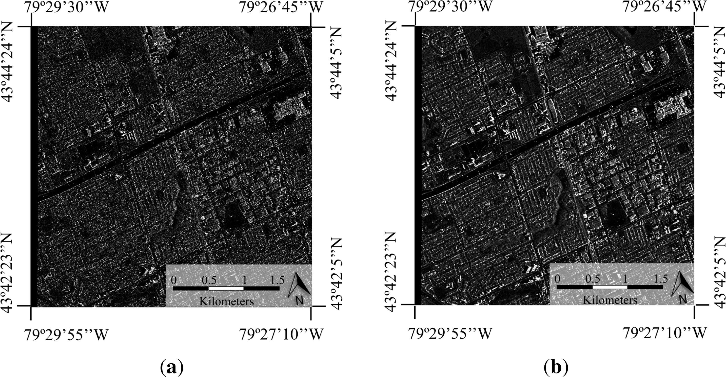
Depending on the geometric resolution, there are two different products: spatially enhanced (SE) and radiometrically enhanced (RE).
SE products are designed for the highest possible square ground resolution. Depending on many parameters, the larger resolution value determines the square pixel size; therefore, the smaller resolution value is adjusted to this size. This equalization of the resolution results in a reduction of the bandwidth, used for speckle reduction.
RE products are optimized with respect to radiometry, decreasing both range and azimuth resolutions to reduce speckle and obtain a radiometric resolution of about 1.5 dB. The result is a product with an equivalent number of looks in the order of five to seven.
Figure 1 includes an example of each of these two products generated from the same SAR image of Toronto (image downloaded from the Infoterra free data website).
2.1.3. Geometric Projection and Data Representation
TerraSAR-X offers four basic products depending on the geometric projection and data representation: single look slant range complex (SSC), multi-look ground range detected (MGD), geocoded ellipsoid corrected (GEC) and enhanced ellipsoid corrected (EEC).
The SSC is the basic single look product of the focused radar signal, where data are represented as complex numbers. The geometric projection is done in the time domain.
The MGD is a detected multi-look product with reduced speckle and square resolution cells on the ground. The image is oriented along the flight direction, and it is not rotated to a map coordinate system, avoiding interpolation artifacts. The consequence of this lack of rotation is that the pixel localization accuracy is lower than in geocoded products.
The GEC is also a multi-look detected product, like the MGD; however, the image is rotated in this case. It is projected and resampled to the WGS84 reference ellipsoid, but no terrain correction is performed. Instead of considering a digital elevation model (DEM), it is assumed for the whole image an average terrain height, resulting in a pixel location accuracy dependent on the terrain.
Once more, the EEC is a multi-look detected product, and like the GEC, it is projected and resampled to the WGS84 reference ellipsoid. The difference with the latter is that terrain-induced distortions are corrected using a DEM in this case. Thus, the pixel localization is highly accurate.
3. Data Set Description
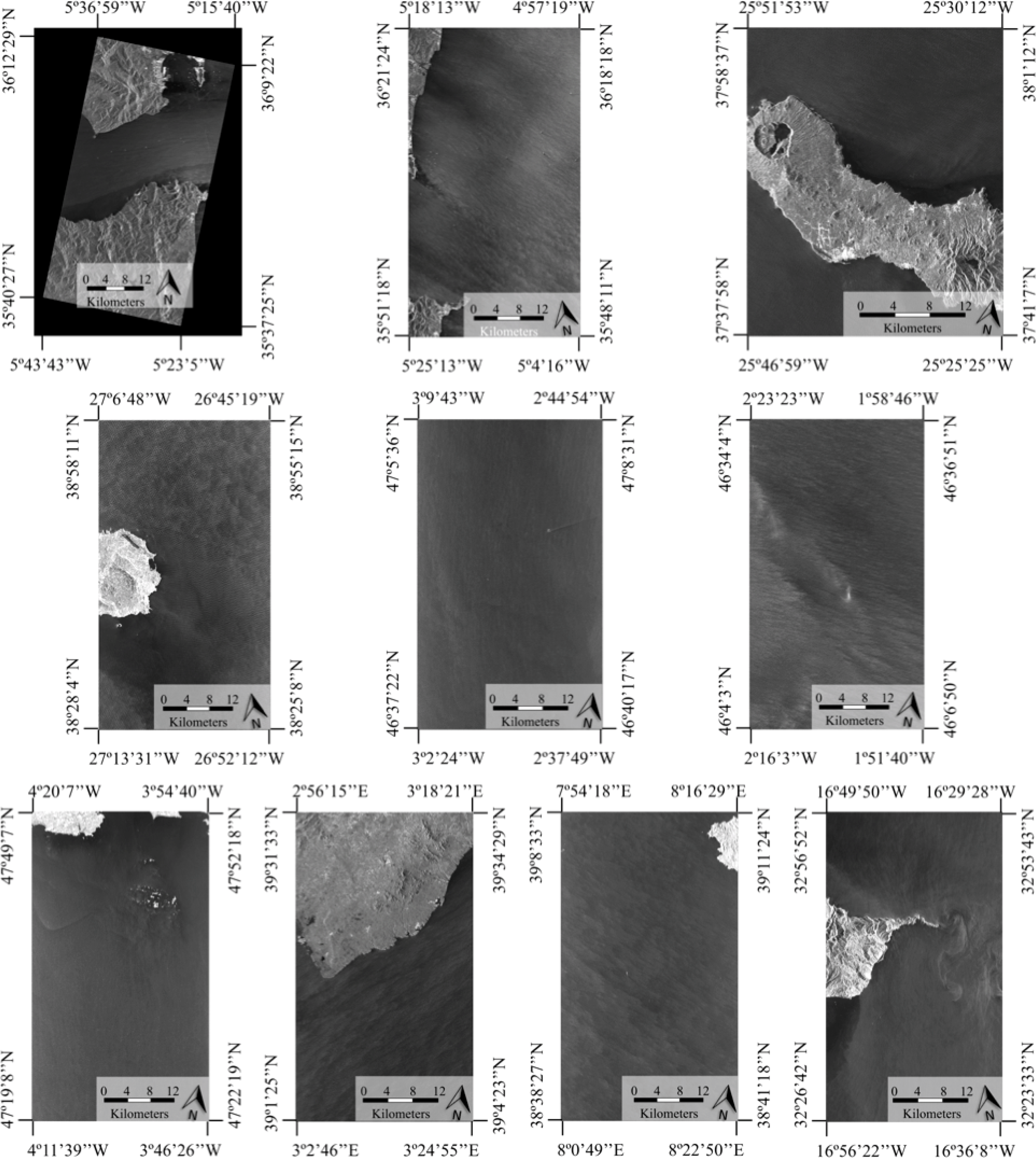
Ten SAR images acquired by TerraSAR-X are used in this paper in order to perform a sea state classification. The quick looks of these images are presented in Figure 2. All of these images are selected for having large sea areas with different characteristics, which may give an idea of the variability of the ocean in SAR images. All of them have in common the acquisition mode and the geometric resolution configuration, so that ground and azimuth resolutions are the same in all images, allowing us to use patches of the same size extracted from any image. Some other acquisition parameters of each image are presented in Table 2. All of the MGD images were provided by the German Aerospace Center under Project COA0158, while the GEC image was downloaded from the Infoterra free data site. The SM mode is selected so that a compromise between the resolution and the scene extent is achieved. As for the geometric resolution, all of the images are SE in order to have the best resolution an SM product can provide, as well as having a square resolution. Furthermore, it must be noted that all of the images share the same polarization (HH), as most of them were acquired under Project COA0158, conceived as a study of the ocean surface, where fusion of data acquired by TerraSAR-X and a marine radar was intended. Since ordinary X-Band marine radars scan the water surface with HH polarization, which is useful to analyze different aspects of the sea surface as ocean waves, wind fields or ocean currents, all of them aspects that determine the sea state [27], SAR images with the same polarization were acquired for this project. In [28], the ocean wave imaging by SAR is studied and compared with data acquired by the marine radar, WaMoS (Wave and Surface Current Monitoring System). Moreover, considering a potential target detection application, where the signal-to-clutter ratio (SCR) is crucial, HH polarization is recommended, as the SCR is improved with respect to VV polarization, and the backscatter signal presents a stronger modulation [29]. However, a study of the effect that the polarization has on the statistical distribution of SAR sea clutter is not overlooked and will be considered in future works.
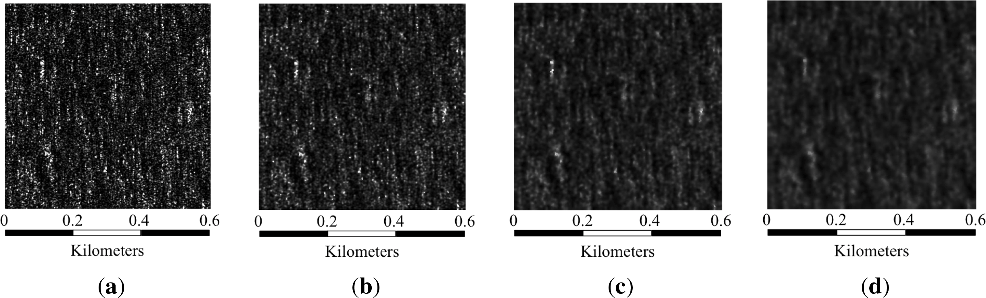
From all of these images, an important number of patches needs to be extracted in order to perform a proper classification. The patch extraction methodology consists of tiling the sea areas of the images into non-overlapping patches. In [10], a study of the ideal patch size was carried out focusing on land areas. For images with a resolution comparable to that of the images selected in this work, the authors proposed a patch size of 160 × 160 pixels. The main difference between land and sea areas is the presence of human structures and the variability of the terrain. Due to these characteristics, the size of the patches needs to be smaller when considering land areas than when working with sea areas. Furthermore, the correlation length of sea clutter has to be accounted for. Since this length depends strongly on the sea state, horizontal and vertical correlations have been measured for different areas of the aforementioned SAR images. Provided that most of the selected areas have vertical or close to vertical wave fields, the horizontal correlation represents in this case the limiting parameter, with values around 100–120 pixels. Therefore, the patch size should be greater than that value. Three patch sizes are considered at first: 150 × 150 pixels, 300 × 300 pixels and 500 × 500 pixels. Considering the resolution of the selected images, these sizes in pixels correspond to approximately 187.5 × 187.5 square meters, 375 × 375 square meters and 625 × 625 square meters, respectively. Different examples are shown in Figure 3.
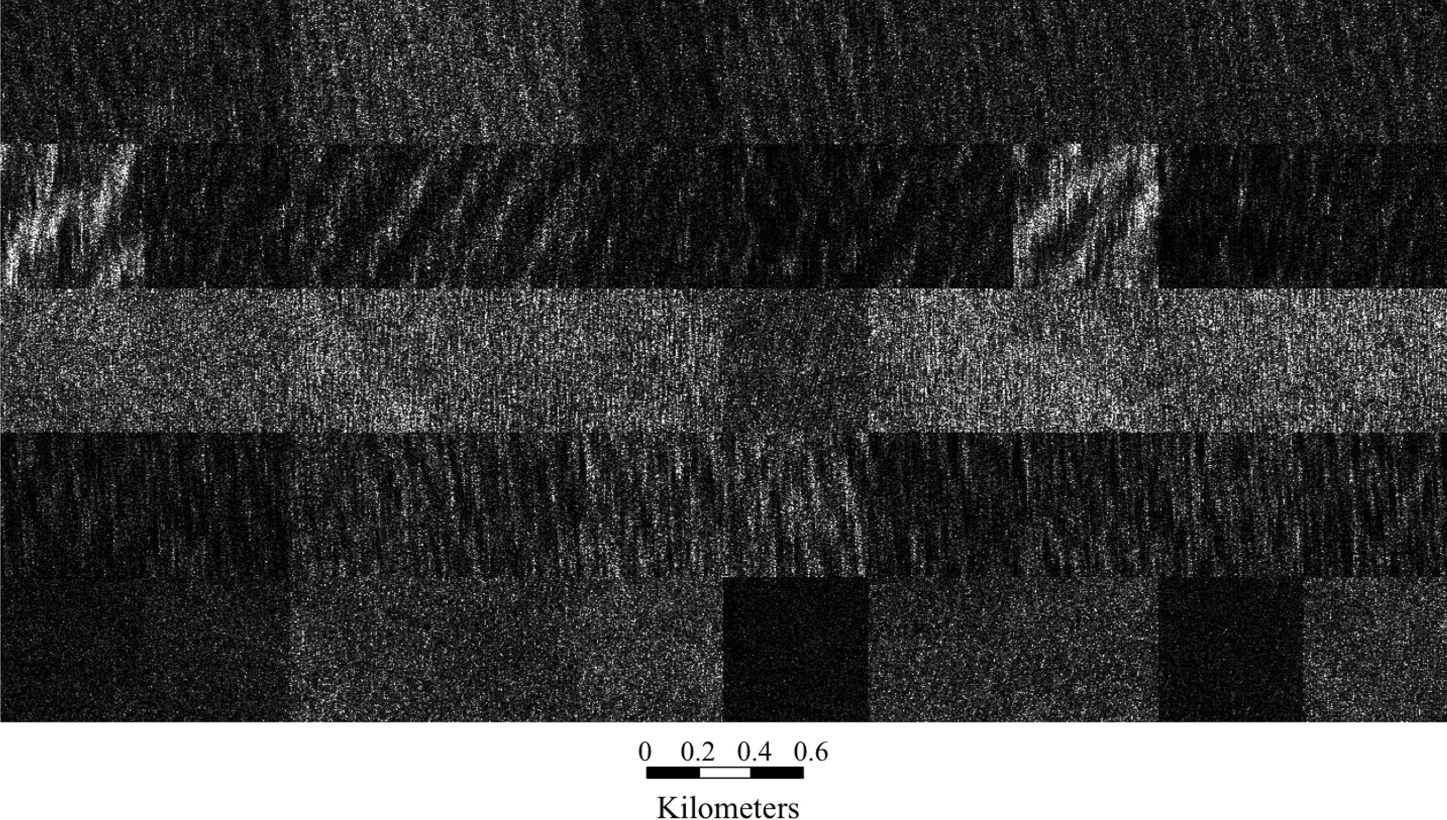
After tiling the sea areas of the 10 images into the three patch sizes, the three data sets are formed by 8100 patches. Now, the data sets are constructed, and the next step is the definition of the classes by visual inspection of the patches. Five classes are defined with the following characteristics:
First class: wave fields with low to medium height waves and different wavelengths. The difference in gray level between the crest and the trough is not very high, meaning both are at medium levels (Figure 4, first row).
Second class: wave fields with high waves and different wavelengths. In this case, the difference in gray level between the crest and the trough is higher than in the first class. Crests tend to be closer to white and troughs closer to black (Figure 4, second row).
Third class: a linear and very narrow structure is visible. This structure does not respond to wave fields (Figure 4, third row).
Fourth class: wave fields where crests and troughs are only partially defined. In classes one and two, crests and troughs describe a linear pattern, but in this class, they hardly appear to be linear (Figure 4, fourth row).
Fifth class: no wave fields or other structure visible. The distribution of the gray level of pixels does not follow any pattern (Figure 4, fifth row).
In Section 7, a study of the best patch size depending on several parameters, such as the classifier, the statistical parameters set and the presence of a speckle filter, will be presented. In Figure 3, where patches from different classes are shown, wave fields come to be more noticeable as the patch size increases, so better success rates are expected for the largest size.
4. Speckle Filtering
Conventional image filtering techniques, such as mean and median filtering, other adaptive filtering techniques, like the Lee [30], Kuan [31], Frost [32] or Lee-Sigma [33] techniques, and new versions of these filters [34] have been proposed to reduce speckle noise. Most of them use a defined filter window to estimate the local noise variance (NV) of a speckled image and perform an individual filtering process. The result is generally a high reduction of speckle noise in areas that are homogeneous, but the image is oversmoothed due to losses in details and edges in heterogeneous areas. Other successful despeckling techniques are based on the Wiener filter and the discrete cosine transform (DCT) [35–37]. The Wiener filter is specially suitable for speckle suppression, due to the consideration that the autocorrelation of speckle in SAR images is not negligible for non-zero lags.
Wavelet-based denoising algorithms have been studied and successfully applied for speckle reduction in SAR images [35,38,39]. These methods perform shrinkage on wavelet coefficients of the SAR image, and some of them apply a preprocessing stage consisting of a logarithmic transformation [40]. A dyadic wavelet decomposition, where speckle is considered as a signal-dependent additive noise and the wavelet coefficients are modeled using the generalized Gaussian and the generalized Gaussian Markov distributions, is presented in [41], outperforming classical filters especially in homogeneous areas. In [42], the application of Donoho wavelet shrinkage denoising techniques [43] in combination with an edge detector was studied to reduce speckle noise, preserving edges and small details in SAR images.
The mean shift (MS) algorithm is a simple nonparametric technique for density gradient estimation proposed by Fukunaga and Hostetler [44] that has been widely used in pattern recognition tasks. In [45], the MS algorithm was introduced in SAR imagery for shadow extraction and building reconstruction, and it was applied along with other parametric filters to single and multi-look synthetic images to detect dark regions. The estimated receiver operating characteristic curves showed that the performance of MS, which requires no assumptions on the statistics, was similar to the performance of the best parametric filter in the considered ideal case. Although the use of MS filtering is not innovative in image processing, its application to SAR images is quite recent, and remarkable results have been achieved. In [46], MS was applied to speckle reduction and edge and texture preservation and also for land mask estimation. The influence of MS parameters was studied and compared to the Lee filter, improving the results of the latter in both speckle noise reduction and edge and texture preservation.
Another filter that has appeared in the last decade is the improved sigma filter [47], which was developed as an improvement to the previous Lee sigma filter implemented by the same author in 1983 [33]. The Lee sigma filter, based on the concept of two-sigma probability, had deficiencies dealing with biased estimation and blurring and depressing strong reflected targets [47], which were more exposed with the advances that SAR technology has experienced in the last two decades. These problems are solved in the improved sigma filter: the sigma range is redefined based on the speckle probability density functions, and a target signature preservation technique is developed in order to mitigate the blurring and depressing.
In this paper, mean shift and the improved sigma filters are considered to study the effect speckle noise has on the statistical distribution of SAR sea clutter. This study is not focused on finding the best speckle filter, and therefore, the decision of using two well-known techniques, such as mean shift and the improved sigma fitter, is based on the fact that both techniques started being applied to SAR imagery in the last decade, achieving remarkable results. Although these two filters are a guarantee to obtain good filtering results, as some of the aforementioned works showed, it cannot be assumed that the results presented in this paper are the best ones, and therefore, a further study focused on the selection of the best speckle filter is highly recommended.
Quality Parameters Estimation
In order to choose the most suitable filter to carry out the speckle filtering, a thorough study of the possible filtering parameters is performed. To evaluate the filters capabilities, three quality parameters are proposed: noise variance (NV), smoothness or equivalent number of looks (ENL) and sharpness. While the first two parameters need to be estimated over a homogeneous area, the third one is measured over the whole image. However, in our case, the patches can be considered homogeneous; therefore, the estimation of the three parameters is done over the whole patches.
The noise variance represents the level of speckle in the image; the more filtered the image, the lower the noise variance value.
The smoothness gives an idea of the equivalent number of looks of the resulting filtered image:
where μ and σ are the mean and the standard deviation values of the considered image, respectively.The sharpness represents how well the details and structure of an image are preserved after the application of the filter. While the other two parameters were estimated solely over the filtered image, this parameter requires a comparison of the original and the filtered images. It is given by:
where x is the original image and ŷ is the filtered image. The closer the value of this parameter to the original number of looks, the better the preservation of details and structure in the filtered image.
In Table 3, the results of the quality parameters estimation for some filtering parameter sets applied to three randomly selected patches are presented. The study included more values, and it was performed over a larger number of patches, but only the most relevant ones are shown. Two free parameters are considered in mean shift: hs and hr, the spatial and range bandwidths, respectively. The spatial bandwidth defines the size of the sliding window, while the range one sets the threshold that defines where the Gaussian kernel is applied. For the hs values presented in Table 3 (2, 4 and 6), the corresponding window sizes are 11 × 11, 15 × 15 and 19 × 19, respectively. As for the sigma filter, two free parameters are considered, too: ξ, which is the sigma value, and Tk, a threshold that defines in a first windowing process whether the pixels within the window are considered part of a point target or not. In this case, the filtering window size is kept constant at 9 × 9, as is recommended in [47].
In the case of mean shift filtering, the quality parameters alone can lead to wrong conclusions, as the best results in terms of noise variance and smoothness are generally obtained when both the space and range bandwidths are higher. However, when these two parameters get higher, the resulting image becomes blurry, and most of the details are lost. Therefore, a trade-off between the estimated parameters and the visual inspection has to be considered. According to Table 3, in two of the three presented patches, the second to best quality parameters values are obtained with a combination of hs = 4 and hr = 0.5. In Figure 5, three parameter sets are applied to Patch 3, showing that by visual inspection the better result between the patch filtered with hs = 4 and hr = 0.5 and the one filtered with hs = 6 and hr = 0.5 is the former. With hs = 2 and hr = 0.5, the image is less filtered and the quality parameters are worse, adding to the decision in favor of the hs = 4 and hr = 0.5 combination.
From the sigma side of Table 3, the main conclusion that can be extracted is that the higher the sigma parameter and the threshold, the better the quality parameters values are. For all of the tested patches, the result is the same; therefore, the sigma filter selected to carry out the preliminary experiments in Section 6 is the one with a sigma value of 0.9 and a threshold value of 0.95.
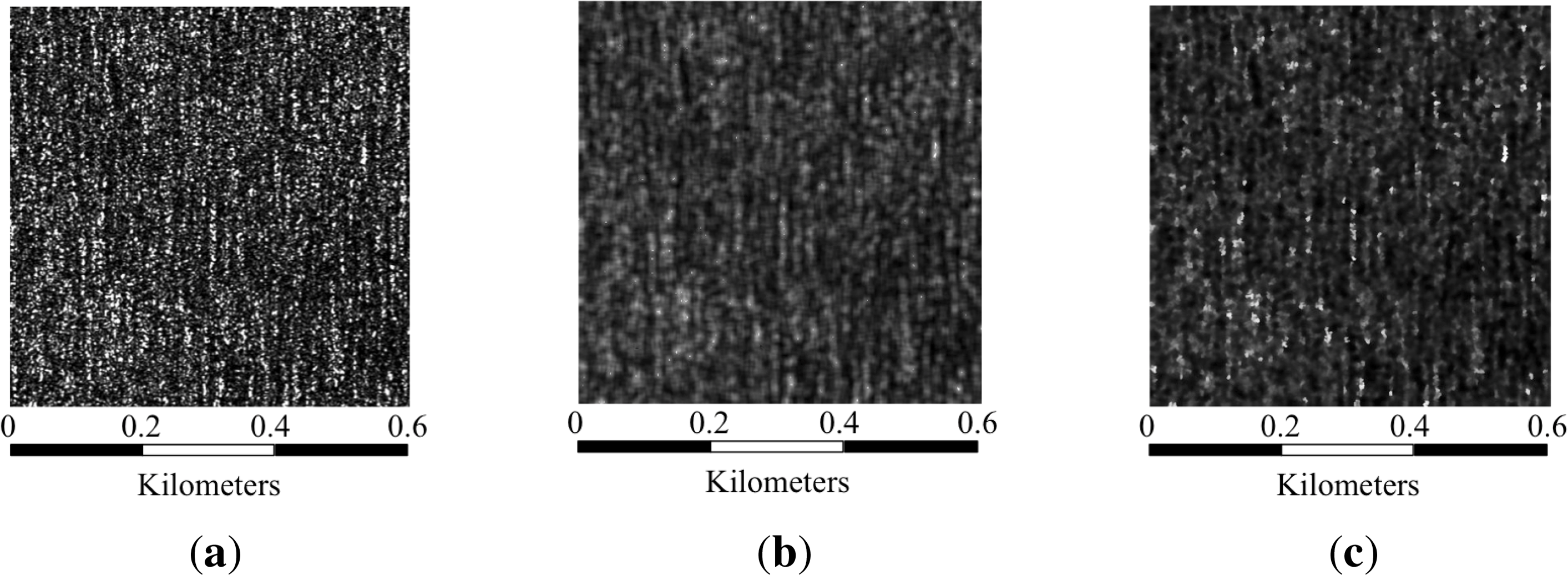
When comparing the selected results of each filter, in most cases, the better results in the quality parameters estimation are attained with mean shift. Moreover, in terms of visual inspection, the mean shift-filtered patches are less blurry than the sigma-filtered ones, as shown in Figure 6, where the original patch is also included for comparison purposes.
5. Statistical Distributions
Plenty of statistical distributions have been studied to model the sea clutter in SAR images with different results. Traditionally, according to the central limit theorem, it has been assumed that the real and imaginary parts of the received data can be modeled by the Gaussian distribution. Although the Gaussian model fits accurately to the low-resolution sea-clutter, it does not perform correctly when the range resolution increases [5]. When dealing with high-resolution SAR systems, such as TerraSAR-X, the application of other distributions is needed. The properties of high-resolution sea-clutter are defined by the surface roughness, which can be characterized by two main types of waves: gravity and capillary waves. Gravity waves describe the macrostructure of the sea surface, with wavelengths from less than a meter to hundreds of meters, while capillary waves have wavelengths of centimeters or less, being caused by surface tension [48]. In order to work with this new high-resolution scenario, other distribution models are typically considered, starting with the Rayleigh model. The Gaussianity of the real and imaginary parts of the received echoes leads to the suitability of this model for the amplitude distribution of the signal. While this model may work fine for some terrain scenes, it may not be the best option for modeling the sea surface, where underlying heavy-tailed distributions might need to be considered instead [4]. Another common distribution used to characterize sea clutter is the K distribution [49], which results from the Rayleigh distribution, used to model the speckle of the received data, and the Gamma distribution, the one that describes the modulation component [4]. Along with the same line of heavy-tailed distributions, the Weibull distribution presents itself as a good option to model both urban scenes and sea clutter [50] and, as does the K distribution, includes the Rayleigh distribution as a special case.
More recently, some other clutter models have emerged to give an answer to the difficulties sea-clutter characterization has. One of the most adopted models for sea-clutter modeling is the generalized gamma distribution, which was first introduced in [51]. Its highly flexible form and good fitting capability have caused this distribution to be applied in different areas, but one of the first to use it for SAR sea-clutter analysis was Anastassopoulos [4]. In the past few years, Li has published many papers dealing with this distribution [52,53]. Although the results visually and quantitatively attained proved that, in most cases, the generalized gamma distribution outperformed the majority of parametric models (Weibull, Nakagami, K and others) in terms of fitting SAR image data histograms, the experiments showed in both papers were applied to different land scenes, but no sea scene was used. In [54], this same distribution is applied to sea images considering different polarizations and sea states, obtaining better results than those obtained by many classic models, including the Gaussian, Log-Normal, Weibull and K.
Another model that has been recently applied is the α-stable distribution, which was first developed for financial time series analysis. It has been used for background clutter modeling in a ship detection scheme proposed by Liao and Wang [55,56], where the images dealt with issues of inhomogeneity and spiky properties. The ability this distribution has to fit heavy-tailed models, due in part to the spiky appearance of inhomogeneous sea-clutter, results in a better modeling performance than the ones obtained by the classical models to which it was compared.
In [9], a special case of this distribution, namely the zero-mean symmetric α-stable (SαS), is used. Along with the generalized central limit theorem, it is assumed that the real and imaginary parts of the received signal are jointly SαS, giving rise to a new model called the generalized heavy-tailed Rayleigh distribution. This new distribution can describe impulsive data and has thicker tails than the classical Rayleigh distribution, allowing a better fit to very-high-resolution (VHR) SAR marine images.
Finally, in [57], the authors address the problem of simultaneous modeling of the joint information by taking a semiparametric approach based on a nonparametric kernel density estimator (KDE) for estimating the marginal distribution and a Gaussian copula to estimate the underlying spatial correlation structure. Results showed that, for the final purpose of the paper, which was ship detection, a significant improvement was achieved in terms of the receiver-operating-characteristic curve and detected target pixels.
Among all of the possible distributions used to model the sea clutter in SAR images, six are considered and compared in this paper: Rayleigh, K, Weibull, gamma, lognormal and generalized gamma. These distributions are selected due to their suitability to model SAR clutter, taking into consideration the geometry of data acquisition by SAR sensors, where incidence angles greater than typical marine radar grazing angles are used. Based on the coherent imaging mechanism of the sensor, it is assumed that each resolution cell contains enough scatterers, whose echoes are independent and identically distributed. Both the amplitude and phase of the echo of one scatterer are statistically random variables. It is also assumed that inside a resolution cell, there are no dominant scatterers, the size of the cell being large enough compared to the size of a scatterer [8]. With these hypotheses acknowledged, many statistical models assume a constant radar cross-section (RCS) background, which leads to a Rayleigh-distributed single-look amplitude and a gamma-distributed multi-look intensity [58]. However, for in-homogeneous regions with underlying gamma-distributed RCS fluctuations, the corresponding intensity data have to be K-distributed. Furthermore, when the resolution becomes high enough, theoretically, the resolution cell will be too small to consider the central limit theorem applicable. In [4], this last assumption is considered leading to the generalized gamma distribution for speckle and intensity RCS fluctuation components. As for the lognormal and Weibull distributions, there is no sound deduction in theory for the suitability of their application to SAR images, as they have come from the experience of having been successfully applied to them [8].
6. Preliminary Statistical Analysis
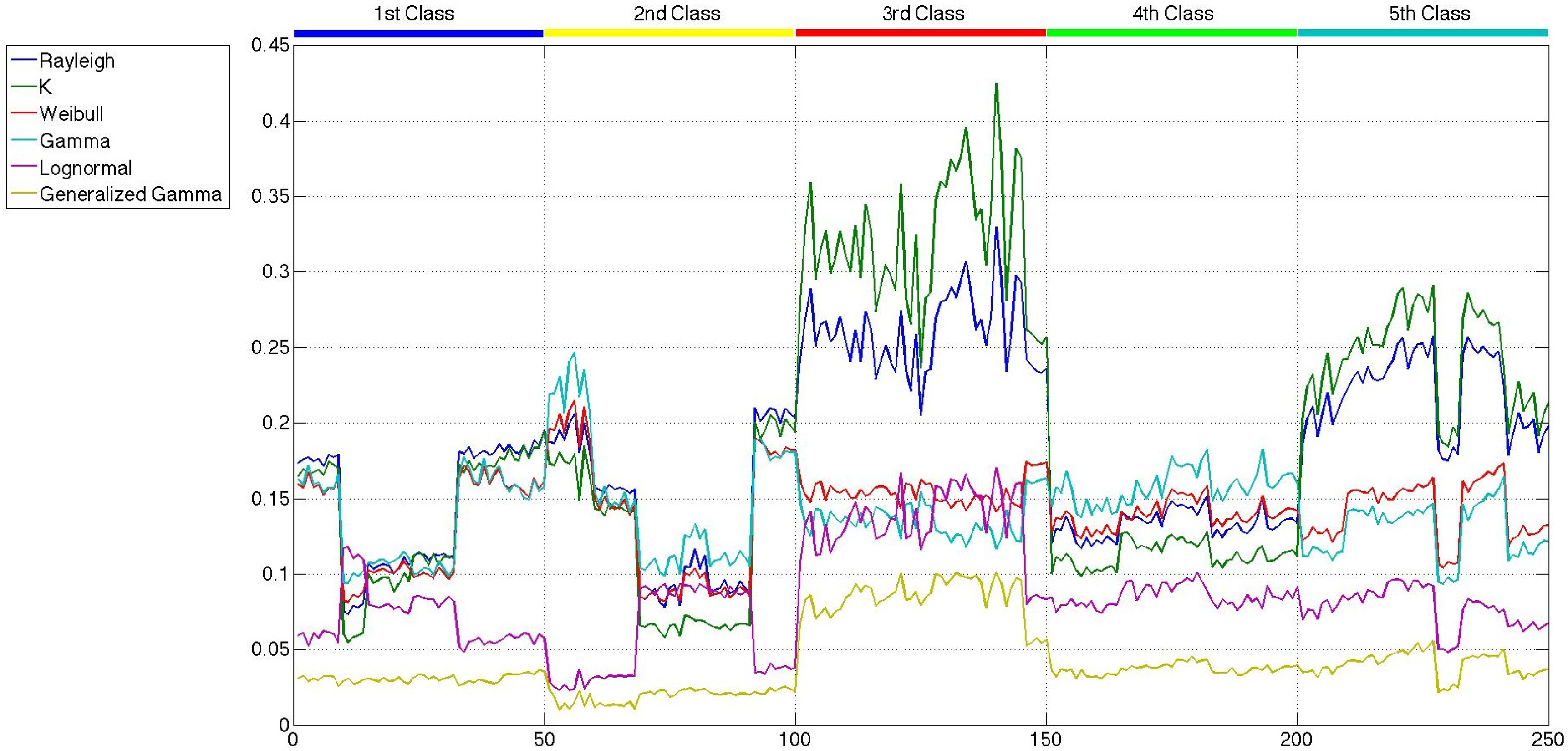
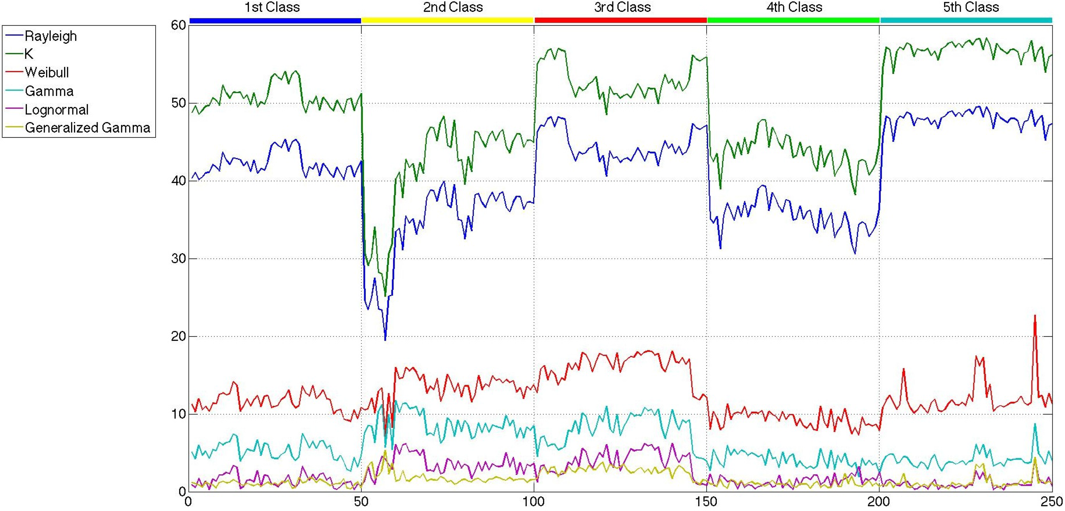
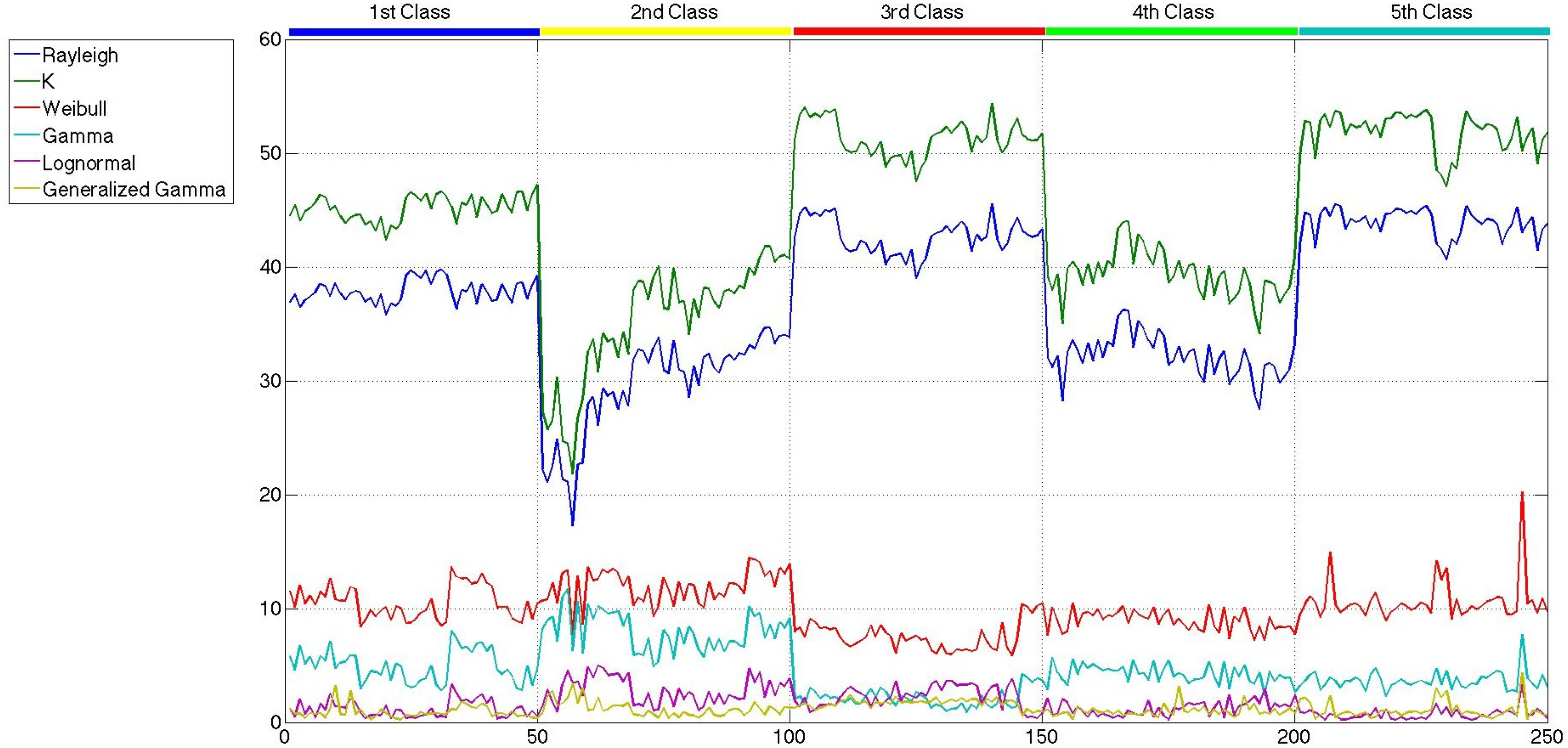
As has been said before, the main goal of this paper is not the modeling of sea clutter, but the classification of sea states. In the previous section, the probability distributions, whose parameters are considered to carry out the classification, were presented. At this point, what is important is how good the parameters classify the sea states and not how good the clutter is modeled. In order to select those parameters, a reduced set of 250,500 × 500-pixel patches is built. Fifty representatives of each class, which are described in Section 3, are taken to build such a set. A first consideration that needs to be addressed is how the application of speckle filtering affects the statistical distribution of the patches, which appears to be reasonable, due to the statistical distribution of speckle itself. In Figures 7 and 9, the lowest values attained for the distances measured with the Cramér–von Mises test [59,60] are shown for the six probability distributions and the 250 patches considered, without speckle filtering, after the mean shift filter and after the sigma filter, respectively. While in all of the figures, the distribution of the patches tends to fit a generalized gamma, the difference between the original patches and the filtered ones is that the distances in the former have several crosses, and in the latter, they are more separated, except for the generalized gamma and the lognormal distributions. If this is translated to how the parameters would be affected by the speckle filters, it is only logical to expect more separation when speckle filtering is applied. There is not much difference between the distances measured for the sigma-filtered and the mean-shift-filtered patches.
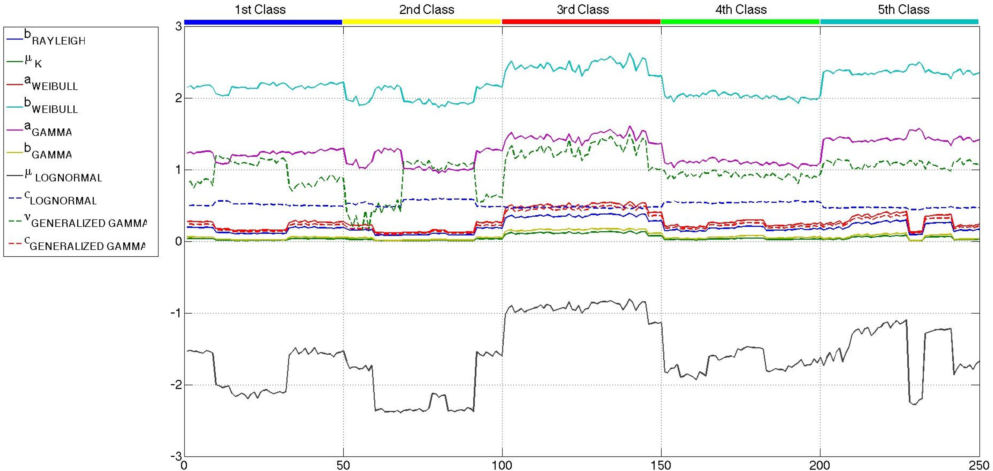
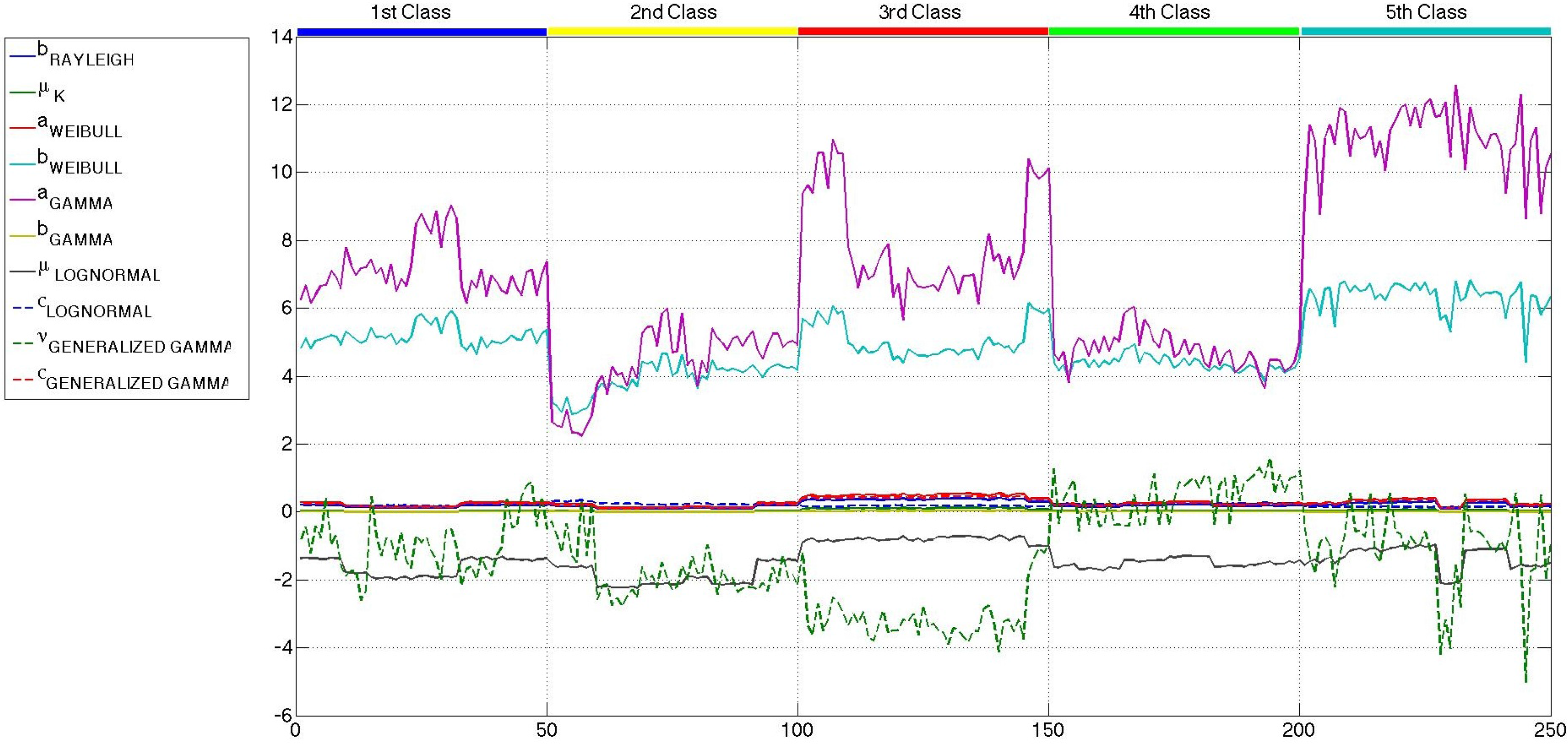
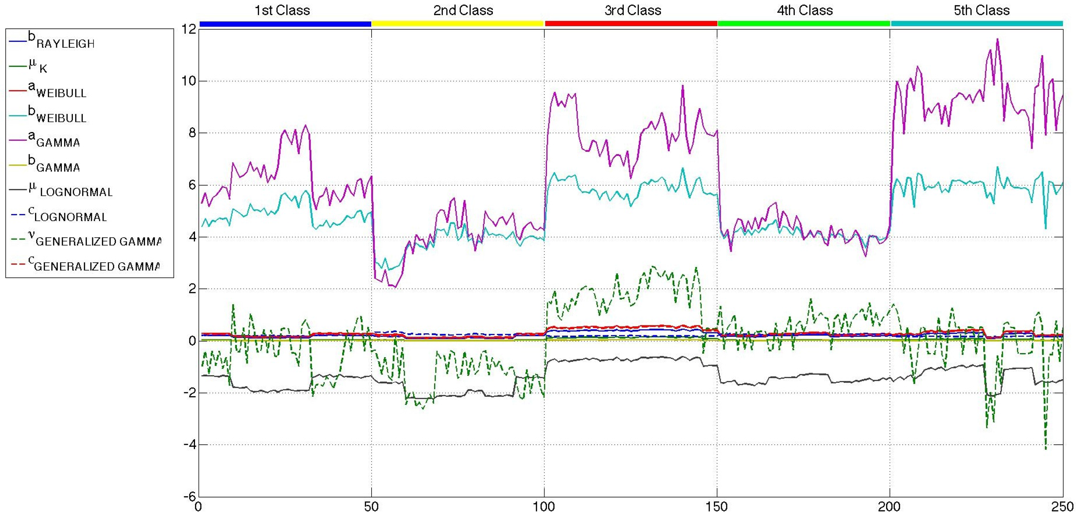
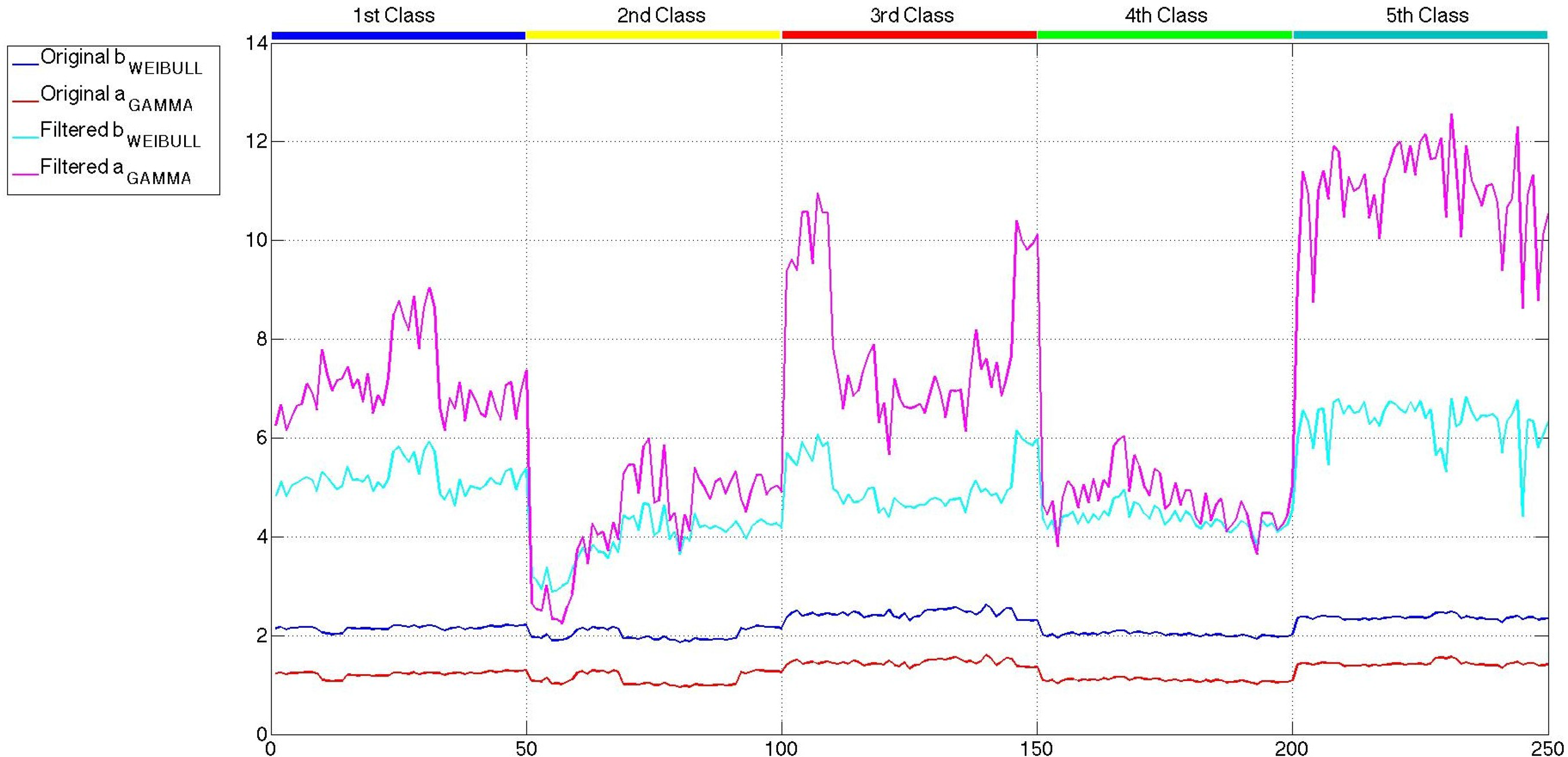
All of the parameters of the six distributions, estimated with the maximum likelihood criterion, are considered at first as candidates to be part of the feature sets used to carry out the classification. However, the values of the shape parameter of the generalized gamma distribution, k, present a huge intra-class variability and inter-classes overlapping, which give rise to confusion when applied to the classifier. Furthermore, it must be noted that the shape parameter of the K distribution has a very low intra-class and inter-classes variability, with no information to discriminate among classes. Therefore, these two parameters are directly excluded from any further consideration, and the other ten are presented in Figures 10 and 12. In this case, the scale of all the parameters is similar, and more conclusions can be extracted.
Comparing the three figures, it is clear that speckle filtering is helping to separate some parameters among the others and also separates between the five classes of patches. In fact, in Figure 13, the parameters that better distinguish between patch classes when speckle filtering is applied are represented for both original and mean-shift-filtered patches, so that a more obvious decision in favor of the application of speckle filtering can be made. These results speak for themselves and show how decisive speckle filtering can be in order to address the classification of the different sea states. Three parameters stand out among the others as the best choices for sea state classification. Those candidates are the shape parameter of the Weibull distribution (bWeibull), the shape parameter of the gamma distribution (aGamma) and the power parameter of the generalized gamma distribution (νGeneralized Gamma). Even though none of them display a perfect separation between classes, the combination of these statistical parameters with others may lead to a nice classification, especially in the case of aGamma, where the thresholds between classes may be more easily selected than with the other parameters. The parameters discarded for classification purposes are mainly the scale ones, which are usually more dependent on the mean level of the patch than the wave field structure. Such dependance would give rise to classes too heterogeneous in terms of wavelength, which is what basically allows the classification. Since the distances and the statistical parameter values for both mean shift and sigma filters are very similar, but the quality parameters presented in Section 4 were slightly better in the case of mean shift, from now on, the studies will only be using this filter with the aforementioned filtering parameters of hs = 4 and hr = 0.5.
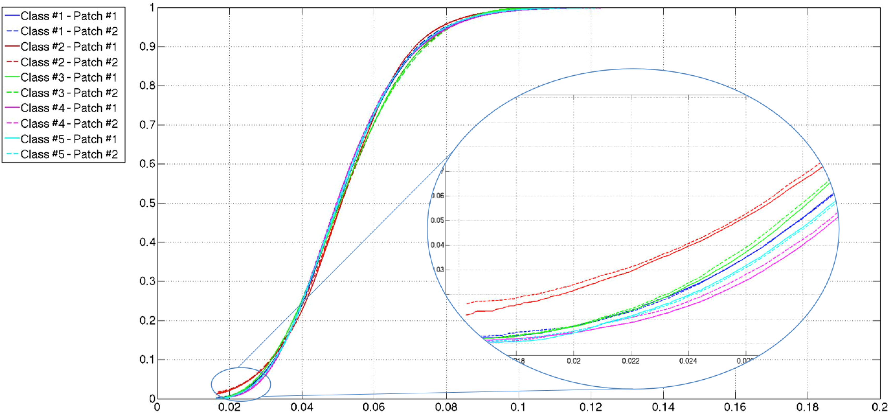
To continue a bit further down this line of thought of exploiting the information provided by the probability distributions, the cumulative distribution functions (cdf) of the patches will be considered. Taking into consideration the way the classes are defined and the role the differences in gray level the wave crests and troughs play, the cdf can provide valuable insight into the percentage of dark and bright pixels. What these values actually represent in a way is the height and depth of crests and troughs, as well as the width of both of them. Given that the shape parameter of the gamma distribution is the one that separates best the five classes, the gamma cdf will be in consideration to estimate the new value. In Figure 14, some cdfs corresponding to patches selected from different classes are presented. Although, at first glance, it looks like all of the curves merge into one, when applying a zoom to the lower values, an interesting separation between the five classes tends to appear. After some study, the third percentile value is selected.
Taking everything into consideration, we define four parameter sets:
Set I: the shape parameter of the gamma distribution and the third percentile of the gamma cdf.
Set II: the shape parameter of the Weibull distribution and the third percentile of the gamma cdf.
Set III: the power parameter of the generalized gamma distribution and the third percentile of the gamma cdf.
Set IV: the shape parameters of the gamma and the Weibull distributions and the third percentile of the gamma cdf.
Many other sets have been considered, starting with the three statistical parameters alone and different combinations of them, but due to space limitations and the poor results achieved with those sets, only the results for the four aforementioned sets will be presented in Section 7.
7. Final Results
The previous sections have been used to describe all of the elements needed for this experimentation section. The SAR images chosen to test the classifiers were introduced in Section 3, and three sets of differently-sized patches were built. The speckle filters that were initially considered in this paper were presented in Section 4, choosing mean shift as the better option. In Sections 5 and 6, six of the most used probability distributions for sea clutter modeling were briefly introduced, and the suitability of their parameters to perform the sea state classification was studied. As a result, four parameter sets were defined. There is one final element needed to complete all of the experiments: the classifier. Four well-known techniques will be compared:
K-means;
Radial basis function neural network (RBFNN);
Nearest neighbor (NN);
Support vector machine (SVM).
These techniques have been widely used in all sorts of applications, not only SAR. Some recent studies with the NN technique were presented in [11], where second-kind statistics were used as classifying features; SVMs have been used in [10,12], comparing them with a supervised Wishart classifier in the latter; in [61], RBFNNs were used for an automatic target recognition application. The K-means classifier is an unsupervised clustering approach. To find the five centroids, the same training set used for the supervised approaches is used. After that, the clusters are formed by measuring the K-means distance between the centroids and the elements in the test set. Furthermore, the first results of K-means clustering were used as a valuable support to first determine which parameters could better separate between the five considered sea state classes.
The experiments that will be carried out will ultimately serve as a comparison in four different levels:
The parameters extracted from the patches;
The patch size;
The classifiers and the number of elements they are composed of in the case of RBFNN and NN;
The absence or presence of a speckle filtering stage.
7.1. Experiments Description
Three sets of patches with different sizes are used to test all of the algorithms. The choice of the size of these patches was explained before in Section 3. Using the largest size to determine the number of elements contained in each set, the number of patches in each class is presented in Table 4.
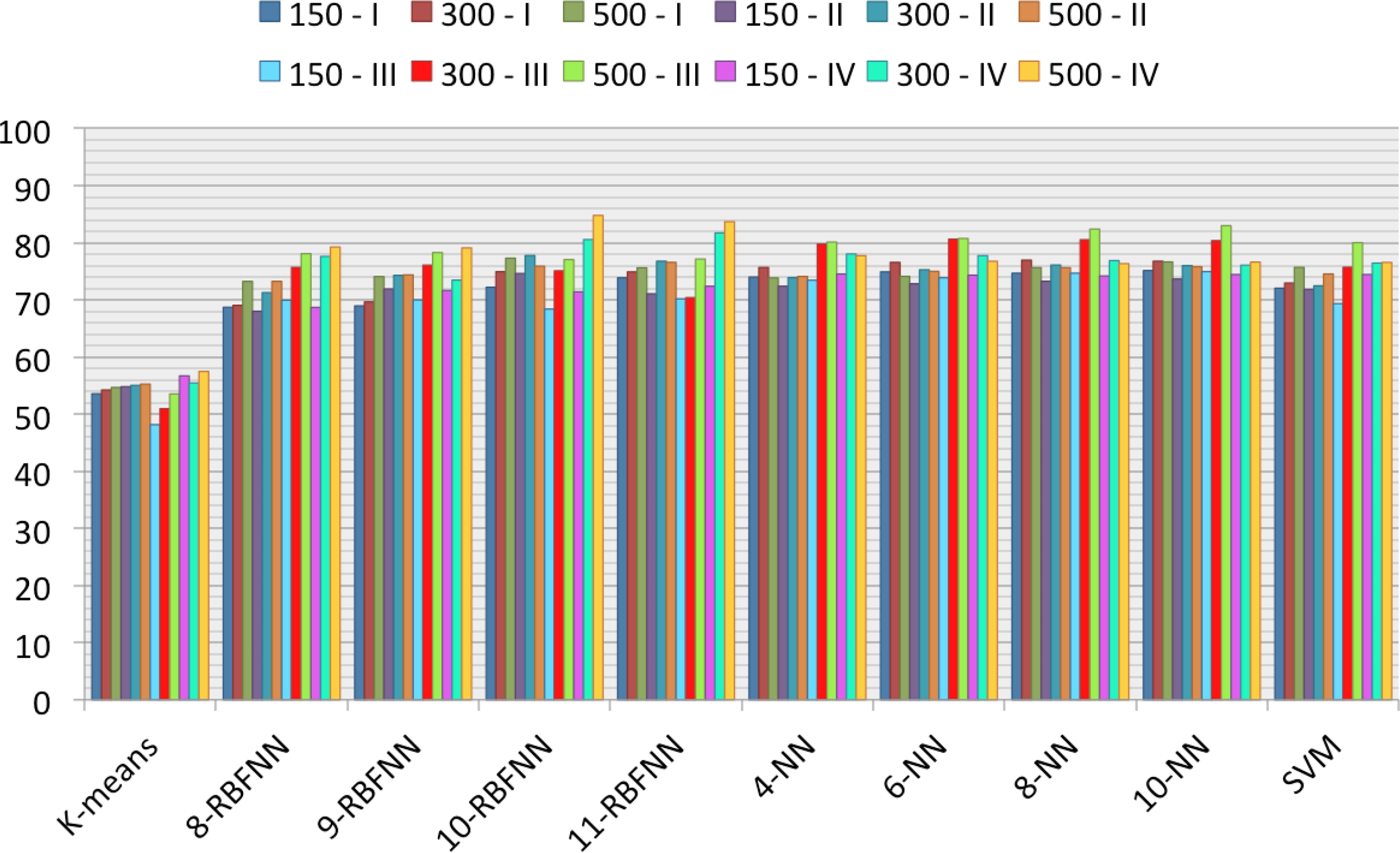
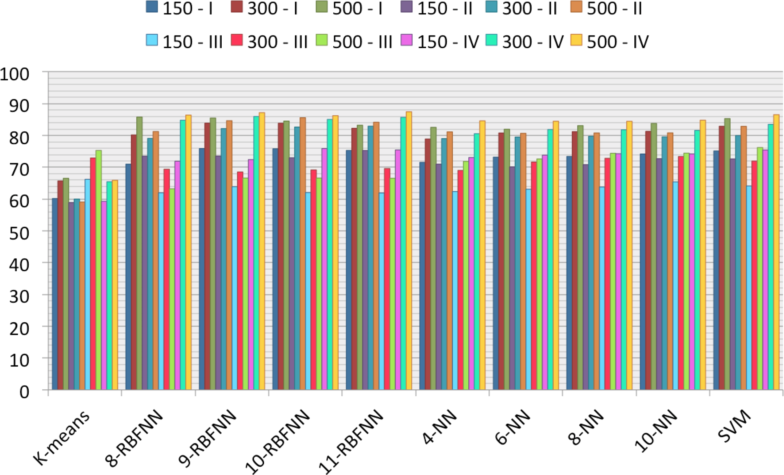
Two hundred fifty patches, 50 of each class, form the set used for training the classifiers, leaving a total of 7850 patches for the test set. All of the success rates presented in the following figures and tables will refer to that test set. In the case of K-means and SVMs, one result is presented for each parameters set (SVMs parameters have been optimized to present the best values), to serve as comparison elements, while a more thorough study is presented for NNs and RBFNNs. For the former, values for 2, 4, 6 and 10 neighbors are presented in Figures 15 and 16, and for the latter, values for 8–11 hidden neurons are presented. The choice of neighbors and hidden neurons presented include the best results and also show the trends of the success rates. The notation used in the figures and tables is k-NN, where k is the number of neighbors, and n-RBFNN, where n is the number of hidden neurons. The success rates as a percentage for the original patches are shown in Figure 15 and for the mean-shift-filtered patches in Figure 16. These results not only are subject to the classifier, but also to the patch size and the parameters set considered. The combination of these two elements represent the different colors of the bars in the figures. Thus, each bar will be denoted by the patch size and the number of the parameter set selected, as seen in Section 6 (e.g., 300-IV represents the combination of a 300 × 300-pixel patch size and parameter set number IV, which includes the shape parameters of the gamma and the Weibull distributions and the third percentile of the gamma cdf).
7.2. Impact of the Speckle Filtering
One of the main purposes of this paper was to give an answer to whether the application of a speckle filter to the SAR images was necessary or not in order to be able to extract more information from the sea clutter and, thus, attain a better classification performance. Preliminary studies, shown in Section 6, suggested the need of a filter, as the statistical parameters began to show potential thresholds between classes when a filter was applied (Figure 13). The results in Figures 15 and 16 confirm what was previously hinted. Globally, the success rates are higher when the speckle filter has been applied, especially for Sets I and II, which included the shape parameter of the gamma distribution and the shape parameter of the Weibull distribution, respectively. Although the best results are attained after applying the speckle filter and a clear improvement of the success rates can be observed, it must be noted that for Set III, the trend is the other way around for most of the classifiers. Let the reader be reminded that this set included the power parameter of the generalized gamma distribution, and while, at first glance, this parameter did not look as promising as others for the classification, the fact that the generalized gamma distribution was the one that best modeled the sea clutter when no speckle filter was applied, as shown in Figure 7, clearly helps to attain these results.
7.3. Patch Size Study
Results presented in Figures 15 and 16 show that in nearly all of the cases studied, the overall success rates reach higher values for a patch size of 500 × 500 pixels, independently of the choice of the parameters set, the classifier and the application of mean shift. Nevertheless, differences are higher when the speckle filter is applied.
The most probable explanation for this behavior is that the 150 × 150-pixel patch is too small to extract enough information on wave fields, which is what mainly allows us to perform the sea state classification. Significantly better results are achieved with a patch size of 300 × 300 pixels, thanks to a better characterization of wave fields. However, the best results are attained with a patch size of 500 × 500 pixels. Even though for some of the experiments, there is not much difference in terms of success rate between 300 × 300 and 500 × 500 patches, global results suggest the selection of the latter.
7.4. Classifier and Parameters Set Selection
When comparing the classifiers, what stands out the most is the inability of the K-means technique to perform the classification. The other three classifiers obtain success rates in the same range, but the RBFNNs are the ones with the best overall performance, except for Set III. As for the number of hidden neurons, there is not a linear evolution of the success rate with the increase in the number of neurons; however, the best results are in most cases attained with 10 or 11 neurons.
Finally, the comparison between parameter sets shows what the first studies in Section 6 already suggested. The shape parameter of the gamma distribution along with the third percentile of gamma cdf outperform the shape parameter of the Weibull distribution and the power parameter of the generalized gamma distribution. However, it is the combination of both shape parameters with the third percentile, that is Set IV, that achieves the best overall results. In concrete terms, the best success rate, with a value of 87.46%, is attained with an RBFNN with 11 hidden neurons (Figure 16). Compared to the result attained under the same conditions, but for the original patches, the improvement is 4%.
7.5. Accuracies, Uncertainties and Errors
The best overall accuracies for each classifier are presented in Table 5 to support with numbers the information shown in Figures 15 and 16. All of them are attained with mean shift-filtered patches, a patch size of 500 × 500 pixels and parameter Set IV, except for K-means, which is parameter Set III. For the RBFNN, 11 hidden neurons have been considered, and for the NN, 10 neighbors. These values show that although K-means can correctly classify three out of four patches, which is far from the results attained by the supervised techniques. The accuracies of these three techniques are close, but it is the RBFNN method that obtains the best results.
In order to add more information, confusion matrices for the experiments with the best overall accuracies are also presented in Tables 6 and 9. These matrices show that the third class is the one with the highest true positives rate for all of the classifiers, with no false negatives in the case of NN and SVM and very low rates of false positives. The fourth class is globally well classified, although over 10% of patches in the second class were classified as the fourth class when RBFNN and NN are used. This issue could be expected, as these two classes correspond to wave fields with high waves. On the other hand, the worst accuracy rate, excluding the results obtained with K-means, which are really low for Classes 1 and 5, is attained with the first class and SVM. In this specific case, almost 16% of the patches are misclassified as the fifth class.
With the information provided by the confusion matrices presented, the unweighted kappa coefficient for each one is calculated (Table 10). This coefficient is a useful statistical measure for assessing the reliability of agreement between a fixed number of classes, which is five in our study. These kappa values confirm the values previously presented for the overall accuracies, as it is the RBFNN with 11 hidden neurons that is the one that attains the value closest to one, and once more, it is K-means that is the technique with the worst result. The value attained for the RBFNN technique, equal to 0.8257, is given for a standard error of kappa of 0.005, with a 95% confidence interval that goes from 0.816 to 0.836.
Taking into consideration the variability of the sea surface and the difficulty a visual classification implies, the results are really good and very encouraging to follow up on these studies to try to find parameters that may improve the final classification success rates even more.
7.6. Computational Complexity
Computational complexity is expressed by two different parameters: the number of CPU cycles and CPU time expressed in seconds. CPU time is calculated by using the number of CPU cycles and an average CPU speed of 2.1605 × 10⁹ cycles/s. The algorithms were executed on a MacBook Pro with OS-X 10.9.4, a 2.2 GHz Intel Core i7 processor, four cores and 8 GB of RAM memory. These algorithms are not parallelized; therefore, the presented values could be reduced if parallel processing was used.
Both CPU times and the number of CPU cycles for speckle filtering, statistical parameters estimation and classification considering one single patch are presented depending on the patch size (Table 11). For the speckle filtering stage, times and cycles for mean shift and sigma, applied to a single patch with the filtering parameters that were selected as the best in Section 4, are presented. The times and cycles for the parameter estimation stage correspond to modeling a single patch with the six statistical distributions described in Section 5, estimating all of the associated parameters. As for the classification algorithms’ times and cycles, since they do not depend on the size of the patch, as the number of parameters extracted from each patch size is the same, one value is presented for each classifier, measured for the cases where the best overall accuracies were attained. These results show that mean shift is faster than sigma, especially when the patch size increases, and the fastest classifier, except for K-means, is the RBFNN. Given that both mean shift and RBFNN attained the best overall results, these times add more value to that achievement.
8. Conclusions
A statistical analysis of Synthetic Aperture Radar sea clutter for sea state classification purposes has been presented in this paper. The lack of studies covering this particular area, as they focus just on the modeling of clutter (either land or sea clutter), served as the motivation to address this topic. The present work successfully used statistical distributions and their parameters to distinguish between different sea states and represents an important contribution to the field, as most SAR classification studies are focused on land areas. Furthermore, a study of the effect speckle noise has on the statistical distribution of sea clutter was carried out, showcasing the necessity of a speckle filtering stage to improve the final classification accuracies.
The importance of the presented work resides not only in the use of statistical distributions for sea state classification and the study of the effect of speckle filtering on the classification accuracy, but also in the extensive resources used to achieve those goals. Ten coastal and maritime SAR images acquired by TerraSAR-X have been selected for this proposal, allowing the construction of a data set with more than 8000 patches and the definition by visual inspection of five sea state classes. For the speckle filtering stage, two filters with well-proven performance results have been used: the improved sigma-Lee filter and the mean shift technique. Six statistical distributions have been studied in this paper: gamma, Weibull, K, Rayleigh, lognormal and generalized gamma. As for the classification stage, four well-known and widely-used classifiers have been considered: K-means, nearest neighbor (NN), radial basis function neural network (RBFNN) and support vector machine (SVM).
The experimental results presented were subjected to a four-level comparison: the effect of speckle filtering, the dependence on the patch size, the statistical parameters sets and the classifiers. Overall classification accuracies for non-filtered and mean-shift-filtered patches, with sizes of 150 × 150, 300 × 300 and 500 × 500 pixels, for four different parameters sets and the aforementioned classifiers were obtained.
Globally, accuracy values experienced an increase when the speckle filter was applied, independently of the parameters set, the patch size and the classifier. The study of the patch size showed that in nearly all cases, the overall accuracies reached higher values for a patch size of 500 × 500 pixels, as more information of the wave fields can be extracted from patches with this size. The parameters set that attained the best classification accuracy values was the one formed by the shape parameters of the gamma and Weibull distributions and the third percentile of the former one; even though the gamma and Weibull distributions were not the best modeling ones, their parameters were indeed the best for sea state classification. As for the classifiers, the three supervised techniques had a similar performance, the RBFNN being the one that slightly stood out as the best. The best result of 87.5% of overall accuracy and the highest kappa coefficient equal to 0.83 were achieved for 500 × 500-pixel patches, filtered with mean shift, the combination of the shape parameter and the third percentile of the gamma distribution, the shape parameter of the Weibull one and a RBFNN with 11 hidden neurons. As an added value, the CPU times of mean shift and the classification based on RBFNN were the best ones among the supervised techniques.
All of the experiments and studies carried out have to be put under the perspective of the resources that have been used. Although a large data set was considered, the extension of the study to a larger number of images could lead to the definition of new sea state classes. Furthermore, the application of the algorithms presented in this paper to data with different resolution and polarization is highly recommended, as a dependence between these parameters and the classification accuracy might be possible. Furthermore, the statistical distribution and the parameters selected to perform the classification can have a big impact on the final results. Many distributions have been considered in this work, but the study of recently applied to SAR distributions, such as the α-stable, is suggested. Results showed that the application of a speckle filter improved the final classification accuracy; therefore, a deeper study of this stage is advised, as well.
The work presented in this paper was first conceived of as a tool for improving ship detection applications in SAR imagery. A lot of effort has been put into this research area in the past few years, as not only researchers, but also governments are interested in the development of maritime surveillance tools. The algorithms and the statistical parameters selected in this work, together with the suggested studies, should be very helpful to perform an automatic ship detector, as most of them are based on the comparison between sea clutter and the target, and the better the clutter modeling, the better the ship detection.
Acknowledgments
This work has been supported by the Spanish “Ministerio de Economía y Competitividad” under Project TEC2012-38701 and University of Alcalá under Project CCG2013/EXP-092.
Most of the data were provided by the German Aerospace Center (DLR) under project “Analysis of Coastal Wave Fields of the Iberian Peninsula using TerraSAR-X Data”, COA0158.
Author Contributions
The database construction, the visual pre-classification and the SAR theory have been developed by Jaime Martin-de-Nicolas, Nerea del-Rey-Maestre and Jose-Luis Barcena-Humanes helped to describe the statistical distributions presented in this paper. David Mata-Moya contributed to the design and training of the machine learning systems used in this paper and along with Maria-Pilar Jarabo-Amores, who supervised the whole work. Finally, the final studies and conclusions were developed by Jaime Martin-de-Nicolas.
Conflicts of Interest
The authors declare no conflicts of interest.
References
- Curlander, J.C.; McDonough, R.N. Synthetic Aperture Radar: Systems and Signal Processing; Wiley-Interscience: Hoboken, NJ, USA, 1991. [Google Scholar]
- Bamler, R. Principles of synthetic aperture radar. Surv. Geophys 2000, 21, 147–157. [Google Scholar]
- Oliver, C.J. Information from SAR images. J. Phys. D Appl. Phys 1991, 24, 1493–1514. [Google Scholar]
- Anastassopoulos, V.; Lampropoulos, G.A.; Drosopulos, A.; Rey, M. High resolution radar clutter statistics. IEEE Trans. Aerosp. Electron. Syst 1999, 35, 43–60. [Google Scholar]
- Carretero-Moya, J.; Gismero-Menoyo, J.; del Campo, A.B.; Asensio-López, A. Statistical analysis of a high-resolution sea-clutter databse. IEEE Trans. Geosci. Remote Sens 2010, 48, 2024–2037. [Google Scholar]
- Chitroub, S.; Houacine, A.; Sansal, B. Statistical characterisation and modelling of SAR images. Elsevier Signal Process 2002, 82, 66–92. [Google Scholar]
- Delignon, Y.; Garello, R.; Hillion, A. Statistical modelling of ocean SAR images. IEE Proc. Radar Sonar Navig 1997, 144, 348–354. [Google Scholar]
- Gao, G. Statistical modeling of SAR images: A survey. Sensors 2010, 10, 775–795. [Google Scholar]
- Kuruoglu, E.; Zerubia, J. Modeling SAR images with a generalization of the rayleigh distribution. IEEE Trans. Image Process 2004, 13, 527–533. [Google Scholar]
- Dumitru, C.O.; Datcu, M. Information content of very high resolution SAR images: Study of feature extraction and imaging parameters. IEEE Trans. Geosci. Remote Sens 2013, 51, 4591–4610. [Google Scholar]
- Singh, J.; Datcu, M. Use of the second-kind statistics for VHR SAR image retrieval. In Proceedings of the 9th International Conference on Communications, Bucharest, Romania, 21–23 June 2012; pp. 367–370.
- Lardeaux, C.; Frison, P.L.; Tison, C.; Souyris, J.C.; Stoll, B.; Fruneau, B.; Rudant, J.P. Support vector machine for multifrequency SAR polarimetric data classification. IEEE Trans. Geosci. Remote Sens 2009, 47, 4143–4152. [Google Scholar]
- Tison, C.; Nicolas, J.M.; Tupin, F.; Maitre, H. A new statistical model for Markovian classification of urban areas in high-resolution SAR images. IEEE Trans. Geosci. Remote Sens 2004, 42, 2046–2057. [Google Scholar]
- Peng, Y.; Chen, J.; Xu, X.; Pu, F. SAR Images statistical modeling and classification based on the mixture of alpha-stable distributions. Remote Sens 2013, 5, 2145–2163. [Google Scholar]
- Wu, S.Y.; Liu, A.K. Towards an automated ocean feature detection, extraction and classification scheme for SAR imagery. Int. J. Remote Sens 2003, 24, 935–951. [Google Scholar]
- Karvonen, J.A. Baltic sea ice SAR segmentation and classification using modified pulse-coupled neural networks. IEEE Trans. Geosci. Remote Sens 2004, 42, 1566–1574. [Google Scholar]
- Soh, L.K.; Tsatsoulis, C. Texture analysis of SAR sea ice imagery using gray level co-occurrence matrices. IEEE Trans. Geosci. Remote Sens 1999, 37, 780–795. [Google Scholar]
- Ochilov, S.; Clausi, D.A. Operational SAR sea-ice image classification. IEEE Trans. Geosci. Remote Sens 2012, 50, 4397–4408. [Google Scholar]
- Martorella, M.; Berizzi, F.; Pastina, D.; Lombardo, P. Exploitation of cosmo skymed SAR images for maritime traffic surveillance. In Proceedings of the IEEE Radar Conference, Kansas City, MO, USA, 23–27 May 2011; pp. 113–117.
- Jarabo-Amores, M.P.; Gonzalez-Bonilla, M.J.; Mata-Moya, D.; de Nicolas, J.M.; Palma-Vazquez, A. Demonstrator of maritime SAR applications: Automatic ship detection results. In Proceedings of the IEEE International Geoscience and Remote Sensing Symposium, Munich, Germany, 22–27 July 2012; pp. 3732–3735.
- Pelich, R.; Longepe, N.; Mercier, G.; Hajduch, G.; Garello, R. AIS-based evaluation of target detectors and SAR sensors characteristics for maritime suerveillance. IEEE J. Sel. Top. Appl. Earth Obs. Remote Sens 2014, 1939–1404. [Google Scholar] [CrossRef]
- Peterson, E.H.; Zee, R.E.; Fotopoulos, G. Wavelet-based despeckling for onboard image processing in a small satellite SAR maritime surveillance constellation. In Proceedings of the IEEE International Geoscience and Remote Sensing Symposium, Munich, Germany, 22–27 July 2012; pp. 1809–1812.
- Margarit, G.; Milanés, J.A.; Tabasco, A. Operational ship monitoring system based on synthetic aperture radar processing. Remote Sens 2009, 1, 375–392. [Google Scholar]
- Liu, A.K.; Hsu, M.K. Deriving ocean surface drift using multiple SAR sensors. Remote Sens 2009, 1, 266–277. [Google Scholar]
- IEEE Aerospace and Electronic Systems Society. In IEEE Standard Radar Definitions 686-2008; IEEE Aerospace and Electronic Systems Society Sponsored by the Radar Systems Panel: New York, NY, USA, 2008.
- Fritz, T.; Eineder, M. TerraSAR-X Ground Segment Basic Product Specification Document; Technical Report; Deutsches Zentrum für Luft- und Raumfahrt DLR: Cologne, Germany, 2013. [Google Scholar]
- Nieto-Borge, J.C.; Jarabo-Amores, M.P.; Mata-Moya, D.; López-Ferreras, F. Estimation of ocean wave heights from temporal sequences of X-Band marine radar images. In Proceedings of the14th European Signal Processing Conference (EUSIPCO), Florence, Italy, 4–8 September 2006.
- Li, X.; Lehner, S.; Rosenthal, W. Investigation of ocean surface wave refraction using TerraSAR-X data. IEEE Trans. Geosci. Remote Sens 2010, 48, 830–840. [Google Scholar]
- Arii, M. Improvement of ship-sea clutter ratio of SAR imagery using standard deviation filter. In Proceedings of the IEEE International Geoscience and Remote Sensing Symposium, Vancouver, BC, Canada, 24–29 July 2011; pp. 632–635.
- Lee, J.S. Digital image enhancement and noise filtering by use of local statistics. IEEE Trans. Pattern Anal. Mach. Intell 1980, PAMI-2, 165–168. [Google Scholar]
- Kuan, D.T.; Sawchuk, A.A.; Strand, T.C.; Chavel, P. Adaptive restoration of images with speckle. IEEE Trans. Acoust. Speech Signal Process 1987, 35, 373–383. [Google Scholar]
- Frost, V.S.; Stiles, J.A.; Shanmugan, K.S.; Holtzman, J.C. A model for radar images and its application to adaptive digital filtering of multiplicative noise. IEEE Trans. Pattern Anal. Mach. Intell 1982, PAMI-4, 157–166. [Google Scholar]
- Lee, J.S. Digital image smoothing and the sigma filter. Comp. Vis. Graph. Image Process 1983, 24, 255–269. [Google Scholar]
- Lu, Y.H.; Tan, S.Y.; Yeo, T.S.; Ng, W.E.; Lim, I.; Zhang, C.B. Adaptive filtering algorithms for SAR speckle reduction. In Proceedings of the IEEE International Geoscience and Remote Sensing Symposium, Lincoln, NE, USA, 27–31 May 1996; pp. 67–69.
- Solbo, S.; Eltoft, T. A stationary wavelet-domain wiener filter for correlated speckle. IEEE Trans. Geosci. Remote Sens 2008, 46, 1219–1230. [Google Scholar]
- Guy, E.V.; Khan, R.H. Three-channel Wiener filter for suppression of speckle noise in SAR images of ocean scenes. In Proceedings of the Canadian Conference on Electrical and Computer Engineering, Halifax, NS, Canada, 25–28 September 1994; 2, pp. 433–436.
- Radford, D.; Kurekin, A.; Marshall, D.; Lever, K. A new DCT-based multiresolution method for simultaneous denoising and fusion of SAR images. In Proceedings of the 9th International Conference on Information Fusion, Florence, Italy, 10–13 July 2006.
- Dai, M.; Peng, C.; Chan, A.K.; Loguinov, D. Bayesian wavelet shrinkage with edge detection for SAR image despeckling. IEEE Trans. Geosci. Remote Sens 2004, 42, 1642–1648. [Google Scholar]
- Xie, H.; Pierce, L.E.; Ulaby, F.T. SAR speckle reduction using wavelet denoising and markov random field modeling. IEEE Trans. Geosci. Remote Sens 2002, 40, 2196–2212. [Google Scholar]
- Argenti, F.; Alparone, L. Speckle removal from SAR images in the undecimated wavelet domain. IEEE Trans. Geosci. Remote Sens 2002, 40, 2363–2374. [Google Scholar]
- Gleich, D.; Datcu, M. Wavelet-based SAR image despeckling and information extraction, using particle filter. IEEE Trans. Image Process 2009, 18, 2167–2184. [Google Scholar]
- Rosa-Zurera, M.; Cóbreces-Álvarez, A.M.; Nieto-Borge, J.C.; Jarabo-Amores, M.P.; Mata-Moya, D. Wavelet denoising with edge detection for speckle reduction in SAR images. In Proceedings of the 15th European Signal Processing Conference, Poznan, Poland, 3–7 September 2007.
- Donoho, D.L. De-noising by soft-thresholding. IEEE Trans. Inf. Theory 1995, 41, 613–627. [Google Scholar]
- Fukunaga, K.; Hostetler, L. The estimation of the gradient of a density function with applications in pattern recognition. IEEE Trans. Inf. Theory 1975, 21, 32–40. [Google Scholar]
- Cellier, F.; Oriot, H.; Nicolas, J.M. Introduction of the mean shift algorithm in SAR imagery: Application to shadow extraction for building reconstruction. In Proceedings of the 1st Earsel 3D Remote Sensing Workshop, Porto, Portugal, 10–11 June 2005.
- Jarabo-Amores, M.P.; Rosa-Zurera, M.; Mata-Moya, D.; Vicen-Bueno, R.; Maldonado-Bascon, S. Spatial-range mean-shift filtering and segmentation applied to SAR images. IEEE Trans. Instrum. Meas 2011, 60, 584–597. [Google Scholar]
- Lee, J.S.; Wen, J.H.; Ainsworth, T.L.; Chen, K.S.; Chen, A.J. Improved sigma filter for speckle filtering of SAR imagery. IEEE Trans. Geosci. Remote Sens 2009, 47, 202–213. [Google Scholar]
- Haykin, S.; Bakker, R.; Currie, B.W. Uncovering nonlinear dynamics—The case study of sea clutter. Proc. IEEE 2002, 90, 860–881. [Google Scholar]
- Jao, J.K. Amplitude distribution of composite terrain clutter and the k-distribution. IEEE Trans. Antennas Propag 1984, 32, 1049–1062. [Google Scholar]
- Sekine, M.; Mao, Y. Weibull Radar Clutter; Preregrinus, P., Ed.; IEE Press: Echternach, Luxembourg, 1990. [Google Scholar]
- Stacy, E.W. A Generalization of the gamma distribution. Ann. Math. Stat 1962, 33, 1187–1192. [Google Scholar]
- Li, H.C.; Hong, W.; Wu, Y.R.; Fan, P.Z. An efficient and flexible statistical model based on generalized gamma distribution for amplitude SAR images. IEEE Trans. Geosci. Remote Sens 2010, 48, 2711–2722. [Google Scholar]
- Li, H.C.; Hong, W.; Wu, Y.R.; Fan, P.Z. On the empirical-statistical modeling of SAR images with generalized gamma distribution. IEEE J. Sel. Top. Signal Process 2011, 5, 386–397. [Google Scholar]
- Qin, X.; Zhou, S.; Gao, G. Statistical modeling of sea clutter in high-resolution SAR images using generalized gamma distribution. In Proceedings of the International Conference on Computer Vision in Remote Sensing, Xiamen, China, 16–18 December 2012; pp. 306–310.
- Wang, C.; Liao, M.; Li, X. Ship detection in SAR image based on the alpha-stable distribution. Sensors 2008, 8, 4948–4960. [Google Scholar]
- Liao, M.; Wang, C.; Wang, Y.; Jiang, L. Using SAR images to detect ships from sea clutter. IEEE Geosci. Remote Sens. Lett 2008, 5, 194–198. [Google Scholar]
- Cui, Y.; Yang, J.; Yamaguchi, Y.; Singh, G.; Park, S.; Kobayashi, H. On semiparametric clutter estimation for ship detection in synthetic aperture radar images. IEEE Trans. Geosci. Remote Sens 2013, 51, 3170–3180. [Google Scholar]
- Oliver, C.; Quegan, S. Understanding Synthetic Aperture Radar Images; SciTech Publishing: Chennai, India, 2004. [Google Scholar]
- Darling, D.A. The kolmogorov-smirnov, cramér-von mises tests. Ann. Math. Stat 1957, 28, 823–838. [Google Scholar]
- Conte, E.; de Maio, A.; Galdi, C. Statistical analysis of real clutter at different range resolutions. IEEE Trans. Aerosp. Electron. Syst 2004, 40, 903–918. [Google Scholar]
- Sun, Y.; Liu, Z.; Todorovic, S.; Li, J. Adaptive boosting for SAR automatic target recognition. IEEE Trans. Aerosp. Electron. Syst 2007, 43, 112–125. [Google Scholar]


| SM | HS | SL | ST | SC | |
|---|---|---|---|---|---|
| Swath width (km) | 30 | 10 | 10 | 7.5 to 4.6 | 100 |
| Product length (km) | 50 | 5 | 10 | 2.5 to 2.8 | 150 |
| Incidence angle range | 20°–45° | 20°–55° | 20°–55° | 20°–45° | 20°–45° |
| Azimuth resolution (m) | 3.3 | 1.1 | 1.7 | 0.24 | 18.5 |
| Ground range resolution (m) | 1.70–3.49 | 1.48–3.49 | 1.48–3.49 | 0.85–1.77 | 1.70–3.49 |
| Product Name | Type | Mode | Geo. | Orbit | Angle | Pol. | Res. | Size |
|---|---|---|---|---|---|---|---|---|
| TSX1_SAR__GEC_SE___SM_S_SRA_20080512T062951_20080512T063000 | GEC | SM | SE | D | 32.2144 | HH | 3 × 3 | 55,600 × 37,600 |
| TSX1_SAR__MGD_SE___SM_S_SRA_20090120T062950_20090120T062958 | MGD | SM | SE | D | 31.0874 | HH | 3 × 3 | 45,333 × 25,289 |
| TSX1_SAR__MGD_SE___SM_S_SRA_20090106T193221_20090106T193226 | MGD | SM | SE | A | 31.0299 | HH | 3 × 3 | 31,086 × 25,806 |
| TSX1_SAR__MGD_SE___SM_S_SRA_20090115T075524_20090115T075532 | MGD | SM | SE | D | 37.3196 | HH | 3 × 3 | 45,254 × 25,194 |
| TSX1_SAR__MGD_SE___SM_S_SRA_20081112T175955_20081112T180003 | MGD | SM | SE | A | 39.2624 | HH | 3 × 3 | 42,474 × 25,479 |
| TSX1_SAR__MGD_SE___SM_S_SRA_20081204T175944_20081204T175952 | MGD | SM | SE | A | 42.8476 | HH | 3 × 3 | 45,118 × 25,492 |
| TSX1_SAR__MGD_SE___SM_S_SRA_20081112T180008_20081112T180016 | MGD | SM | SE | A | 33.2739 | HH | 3 × 3 | 45,234 × 25,848 |
| TSX1_SAR__MGD_SE___SM_S_SRA_20081102T174040_20081102T174048 | MGD | SM | SE | A | 39.2196 | HH | 3 × 3 | 45,213 × 25,958 |
| TSX1_SAR__MGD_SE___SM_S_SRA_20081206T172316_20081206T172324 | MGD | SM | SE | A | 42.8647 | HH | 3 × 3 | 45,179 × 25,911 |
| TSX1_SAR__MGD_SE___SM_S_SRA_20080709T071352_20080709T071400 | MGD | SM | SE | D | 31.0636 | HH | 3 × 3 | 45,360 × 25,807 |
| Patch 1 NVoriginal = 0.8081 EN Loriginal = 1.2375 | |||||||
| Mean Shift | Sigma | ||||||
| NV | ENL | Sharpness | NV | ENL | Sharpness | ||
| hs = 2 hr = 0.2 | 0.8187 | 1.2215 | 3.5636 | ξ = 0.5 Tk = 0.85 | 0.1637 | 6.1104 | 1.8218 |
| hs = 2 hr = 0.5 | 0.4481 | 2.2318 | 4.2543 | ξ = 0.5 Tk = 0.90 | 0.1613 | 6.1985 | 1.8216 |
| hs = 2 hr = 0.8 | 0.3459 | 2.8912 | 4.3460 | ξ = 0.5 Tk = 0.95 | 0.1596 | 6.2659 | 1.8214 |
| hs = 4 hr = 0.2 | 0.7261 | 1.3773 | 2.2625 | ξ = 0.7 Tk = 0.85 | 0.1404 | 7.1204 | 1.7262 |
| hs = 4 hr = 0.5 | 0.1630 | 6.1333 | 2.1122 | ξ = 0.7 Tk = 0.90 | 0.1383 | 7.2321 | 1.7260 |
| hs = 4 hr = 0.8 | 0.1336 | 7.4842 | 2.1014 | ξ = 0.7 Tk = 0.95 | 0.1367 | 7.3178 | 1.7258 |
| hs = 6 hr = 0.2 | 0.6557 | 1.5252 | 1.7824 | ξ = 0.9 Tk = 0.85 | 0.1341 | 7.4558 | 1.7120 |
| hs = 6 hr = 0.5 | 0.0721 | 13.8783 | 1.6507 | ξ = 0.9 Tk = 0.90 | 0.1320 | 7.5763 | 1.7118 |
| hs = 6 hr = 0.8 | 0.0703 | 14.2171 | 1.6627 | ξ = 0.9 Tk = 0.95 | 0.1304 | 7.6687 | 1.7116 |
| Patch 2 NVoriginal = 0.9549 EN Loriginal = 1.0473 | |||||||
| Mean Shift | Sigma | ||||||
| NV | ENL | Sharpness | NV | ENL | Sharpness | ||
| hs = 2 hr = 0.2 | 0.3887 | 2.5728 | 3.7697 | ξ = 0.5 Tk = 0.85 | 0.1886 | 5.3021 | 1.7379 |
| hs = 2 hr = 0.5 | 0.3406 | 2.9359 | 3.7282 | ξ = 0.5 Tk = 0.90 | 0.1886 | 5.3021 | 1.7379 |
| hs = 2 hr = 0.8 | 0.3392 | 2.9478 | 3.6738 | ξ = 0.5 Tk = 0.95 | 0.1886 | 5.3021 | 1.7379 |
| hs = 4 hr = 0.2 | 0.1439 | 6.9500 | 1.8828 | ξ = 0.7 Tk = 0.85 | 0.1664 | 6.0104 | 1.6476 |
| hs = 4 hr = 0.5 | 0.1402 | 7.1342 | 1.9082 | ξ = 0.7 Tk = 0.90 | 0.1664 | 6.0104 | 1.6476 |
| hs = 4 hr = 0.8 | 0.1463 | 6.8358 | 1.9060 | ξ = 0.7 Tk = 0.95 | 0.1664 | 6.0104 | 1.6476 |
| hs = 6 hr = 0.2 | 0.0945 | 10.5805 | 1.5145 | ξ = 0.9 Tk = 0.85 | 0.1595 | 6.2695 | 1.6331 |
| hs = 6 hr = 0.5 | 0.0905 | 11.0553 | 1.5369 | ξ = 0.9 Tk = 0.90 | 0.1595 | 6.2695 | 1.6331 |
| hs = 6 hr = 0.8 | 0.0951 | 10.5154 | 1.5420 | ξ = 0.9 Tk = 0.95 | 0.1595 | 6.2695 | 1.6331 |
| Patch 3 NVoriginal = 1.1922 EN Loriginal = 0.8388 | |||||||
| Mean Shift | Sigma | ||||||
| NV | ENL | Sharpness | NV | ENL | Sharpness | ||
| hs = 2 hr = 0.2 | 0.7299 | 1.3701 | 3.1335 | ξ = 0.5 Tk = 0.85 | 0.2639 | 3.7899 | 1.6069 |
| hs = 2 hr = 0.5 | 0.4969 | 2.0126 | 3.6894 | ξ = 0.5 Tk = 0.90 | 0.2632 | 3.7987 | 1.6069 |
| hs = 2 hr = 0.8 | 0.4774 | 2.0948 | 3.6645 | ξ = 0.5 Tk = 0.95 | 0.2630 | 3.8027 | 1.6069 |
| hs = 4 hr = 0.2 | 0.3630 | 2.7547 | 1.6567 | ξ = 0.7 Tk = 0.85 | 0.2379 | 4.2030 | 1.5212 |
| hs = 4 hr = 0.5 | 0.1853 | 5.3955 | 1.7663 | ξ = 0.7 Tk = 0.90 | 0.2374 | 4.2131 | 1.5212 |
| hs = 4 hr = 0.8 | 0.2005 | 4.9879 | 1.7852 | ξ = 0.7 Tk = 0.95 | 0.2371 | 4.2176 | 1.5212 |
| hs = 6 hr = 0.2 | 0.2683 | 3.7276 | 1.3038 | ξ = 0.9 Tk = 0.85 | 0.2303 | 4.3421 | 1.5081 |
| hs = 6 hr = 0.5 | 0.1084 | 9.2248 | 1.3500 | ξ = 0.9 Tk = 0.90 | 0.2297 | 4.3527 | 1.5081 |
| hs = 6 hr = 0.8 | 0.1232 | 8.1161 | 1.3782 | ξ = 0.9 Tk = 0.95 | 0.2295 | 4.3575 | 1.5081 |
| First Class | Second Class | Third Class | Fourth Class | Fifth Class |
|---|---|---|---|---|
| 2438 | 2998 | 352 | 1858 | 454 |
| K-Means | 11-RBFNN | 10-NN | SVM |
|---|---|---|---|
| 75.3090 | 87.4634 | 84.8261 | 86.5588 |
| Predicted Class | 1st | 2nd | 3rd | 4th | 5th |
|---|---|---|---|---|---|
| Actual Class | |||||
| 1st | 45.6030 | 27.7219 | 0.5025 | 20.1843 | 5.9883 |
| 2nd | 3.3582 | 90.6377 | 0 | 6.0041 | 0 |
| 3rd | 0 | 0 | 93.0233 | 0 | 6.9767 |
| 4th | 3.0973 | 2.5442 | 0 | 94.2478 | 0.1106 |
| 5th | 37.1287 | 15.0990 | 0.2475 | 6.4356 | 41.0891 |
| Predicted Class | 1st | 2nd | 3rd | 4th | 5th |
|---|---|---|---|---|---|
| Actual Class | |||||
| 1st | 86.5578 | 0.7956 | 2.3451 | 6.1977 | 4.1039 |
| 2nd | 6.0719 | 83.2090 | 0 | 10.7191 | 0 |
| 3rd | 0.6645 | 0 | 99.3355 | 0 | 0 |
| 4th | 3.6504 | 1.7146 | 0 | 94.6350 | 0 |
| 5th | 14.8515 | 1.7327 | 0.2475 | 0.2475 | 82.9208 |
| Predicted Class | 1st | 2nd | 3rd | 4th | 5th |
|---|---|---|---|---|---|
| Actual Class | |||||
| 1st | 83.6265 | 0.9213 | 3.4757 | 6.0720 | 5.9045 |
| 2nd | 6.4111 | 79.2062 | 0 | 14.3826 | 0 |
| 3rd | 0 | 0 | 100 | 0 | 0 |
| 4th | 3.6504 | 4.0376 | 0 | 92.3119 | 0 |
| 5th | 10.6436 | 0.4950 | 0.2475 | 0.4950 | 88.1188 |
| Predicted Class | 1st | 2nd | 3rd | 4th | 5th |
|---|---|---|---|---|---|
| Actual Class | |||||
| 1st | 74.8744 | 0.4188 | 2.2613 | 6.7420 | 15.7035 |
| 2nd | 4.7151 | 91.0448 | 0 | 4.2062 | 0.0339 |
| 3rd | 0 | 0 | 100 | 0 | 0 |
| 4th | 3.1527 | 5.8628 | 0 | 90.7633 | 0.2212 |
| 5th | 5.1980 | 0.2475 | 0.2475 | 0.2475 | 94.0594 |
| K-Means | 11-RBFNN | 10-NN | SVM |
|---|---|---|---|
| 0.6511 | 0.8257 | 0.7904 | 0.8146 |
| CPU Cycles | CPU Time (s) | |||||
|---|---|---|---|---|---|---|
| Patch size | 150 × 150 | 300 × 300 | 500 × 500 | 150 × 150 | 300 × 300 | 500 × 500 |
| Mean Shift | 4,705,897,519 | 15,991,855,606 | 43,105,229,247 | 2.1782 | 7.4019 | 19.9515 |
| Sigma | 23,438,933,492 | 70,384,918,352 | 183,524,472,102 | 10.8488 | 32.5781 | 84.9454 |
| Parameter estimation | 47,655,839 | 124,194,090 | 324,481,363 | 0.0221 | 0.0575 | 0.1502 |
| K-means | 35,908 | 0.000017 | ||||
| RBFNN | 285,932 | 0.000132 | ||||
| NN | 4,015,497 | 0.001859 | ||||
| SVM | 6,337,956 | 0.002934 | ||||
© 2014 by the authors; licensee MDPI, Basel, Switzerland This article is an open access article distributed under the terms and conditions of the Creative Commons Attribution license (http://creativecommons.org/licenses/by/4.0/).
Share and Cite
Martín-de-Nicolás, J.; Jarabo-Amores, M.-P.; Mata-Moya, D.; Del-Rey-Maestre, N.; Bárcena-Humanes, J.-L. Statistical Analysis of SAR Sea Clutter for Classification Purposes. Remote Sens. 2014, 6, 9379-9411. https://doi.org/10.3390/rs6109379
Martín-de-Nicolás J, Jarabo-Amores M-P, Mata-Moya D, Del-Rey-Maestre N, Bárcena-Humanes J-L. Statistical Analysis of SAR Sea Clutter for Classification Purposes. Remote Sensing. 2014; 6(10):9379-9411. https://doi.org/10.3390/rs6109379
Chicago/Turabian StyleMartín-de-Nicolás, Jaime, María-Pilar Jarabo-Amores, David Mata-Moya, Nerea Del-Rey-Maestre, and José-Luis Bárcena-Humanes. 2014. "Statistical Analysis of SAR Sea Clutter for Classification Purposes" Remote Sensing 6, no. 10: 9379-9411. https://doi.org/10.3390/rs6109379