Improved Accuracy of Chlorophyll-a Concentration Estimates from MODIS Imagery Using a Two-Band Ratio Algorithm and Geostatistics: As Applied to the Monitoring of Eutrophication Processes over Tien Yen Bay (Northern Vietnam)


Abstract
:
1. Introduction
2. Materials
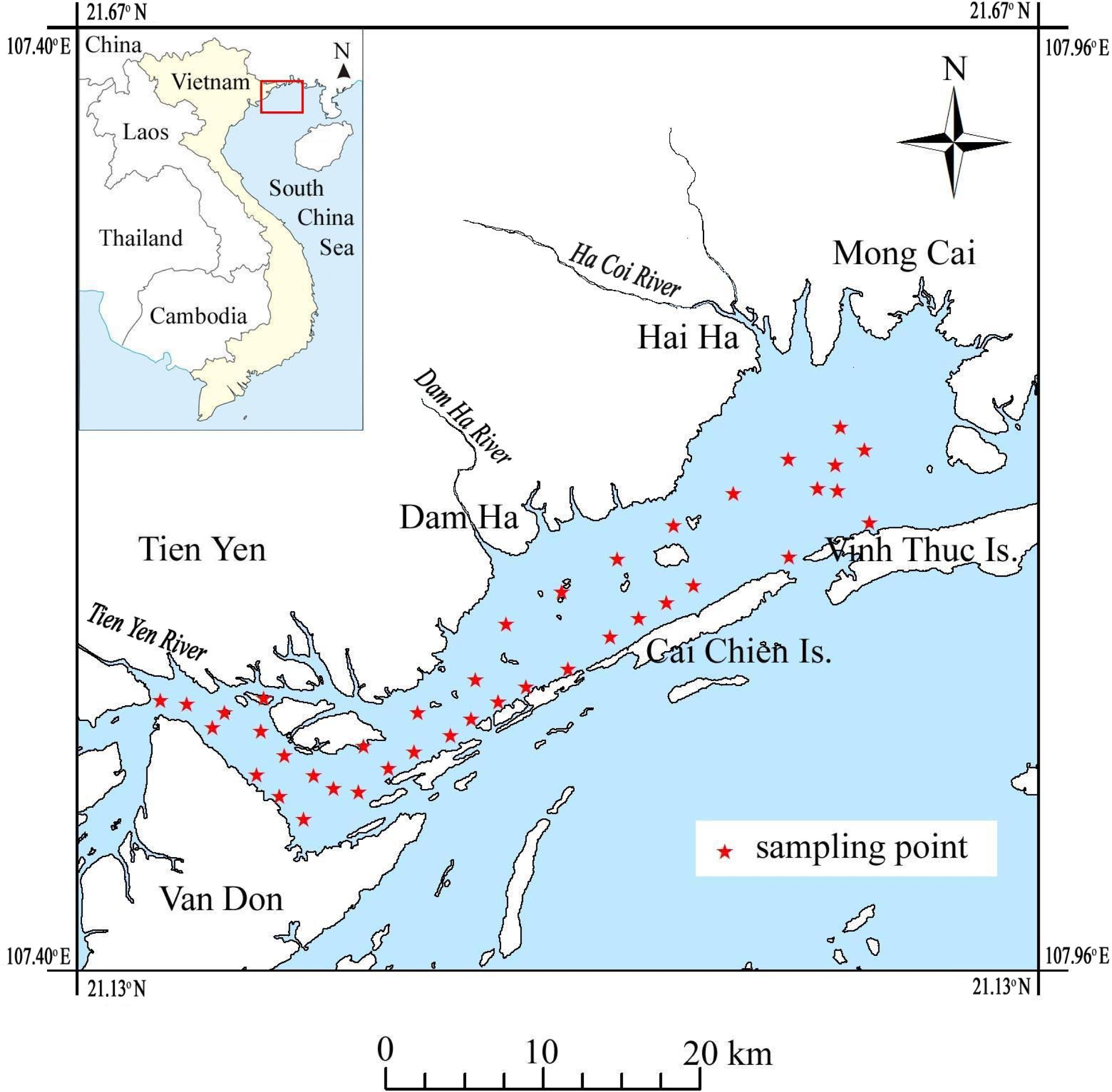
2.1. Features of the Study Area
2.2. Collection of Sample Data
2.3. MODIS Image Data
3. Methods for Estimating Chl-a Concentration
3.1. Review of Estimation Algorithms
3.2. New Algorithm Development
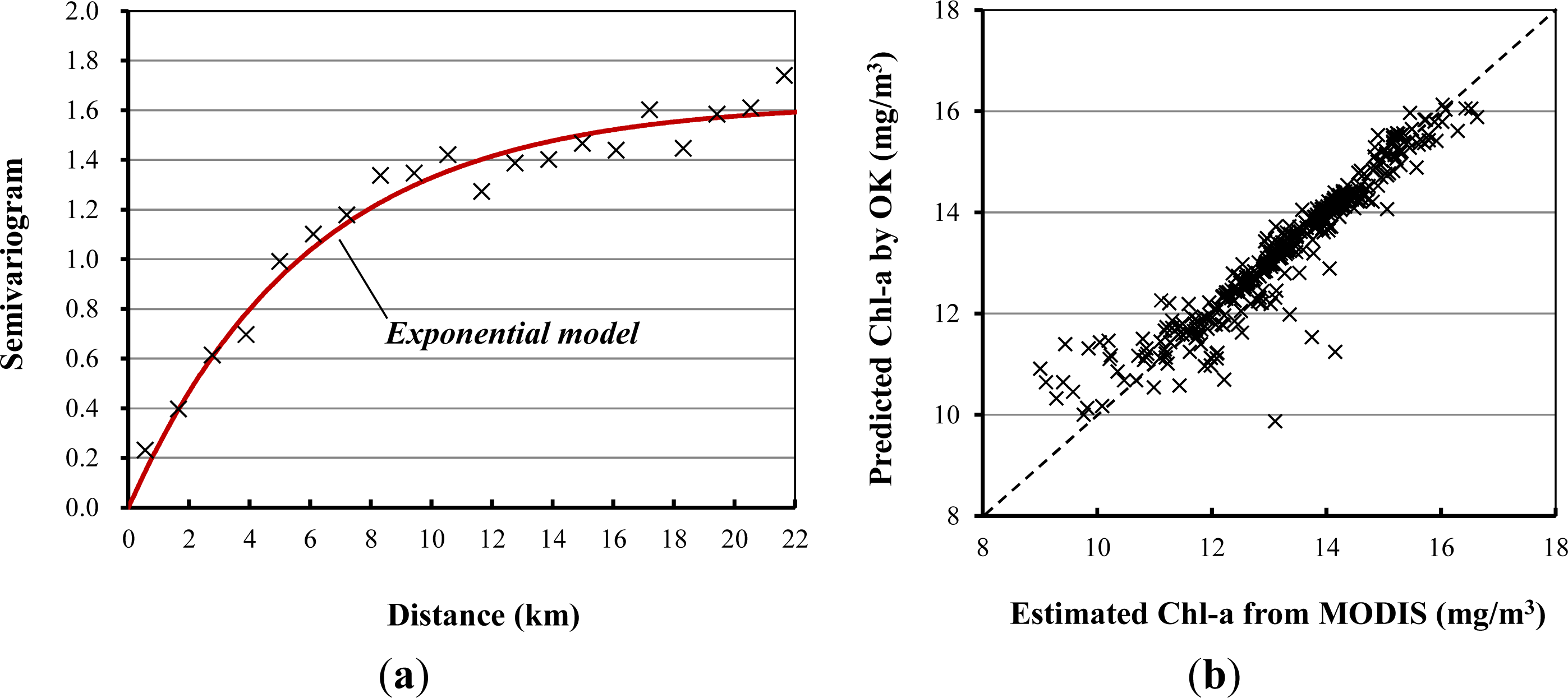
3.3. Geostatistical Methods
4. Results and Discussion
4.1. Atmospheric Correction
4.2. Estimation Algorithm for Chl-a Concentrations
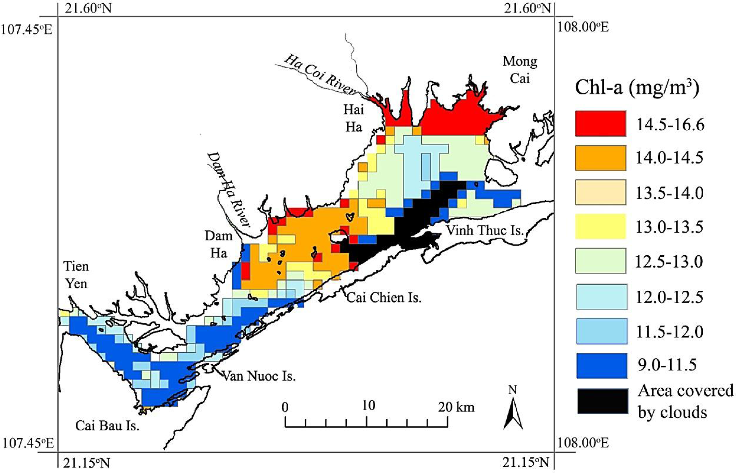
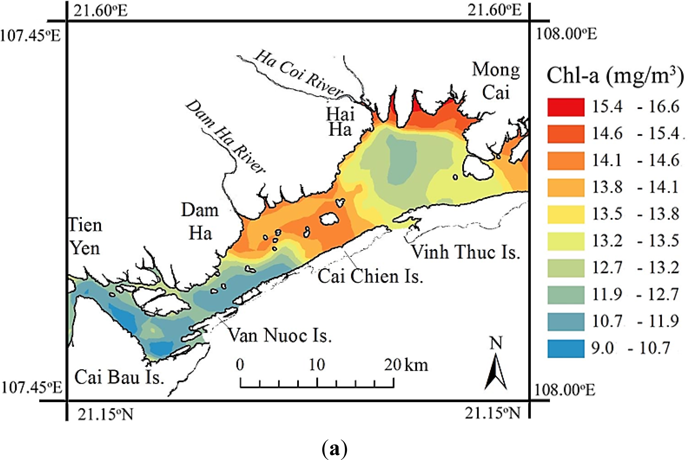
4.3. Spatial Distribution of Chl-a Concentrations
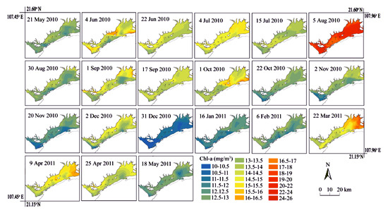
4.4. Eutrophication Processes over the Course of a Year
5. Conclusions
- (1)
- Two widely-used atmospheric correction methods, DOS and QUAC, were compared to obtain reflectance at the sea surface by excluding atmospheric contributions from the MODIS image data. DOS was identified to be more suitable for tropical waters, such as those of Tien Yen Bay.
- (2)
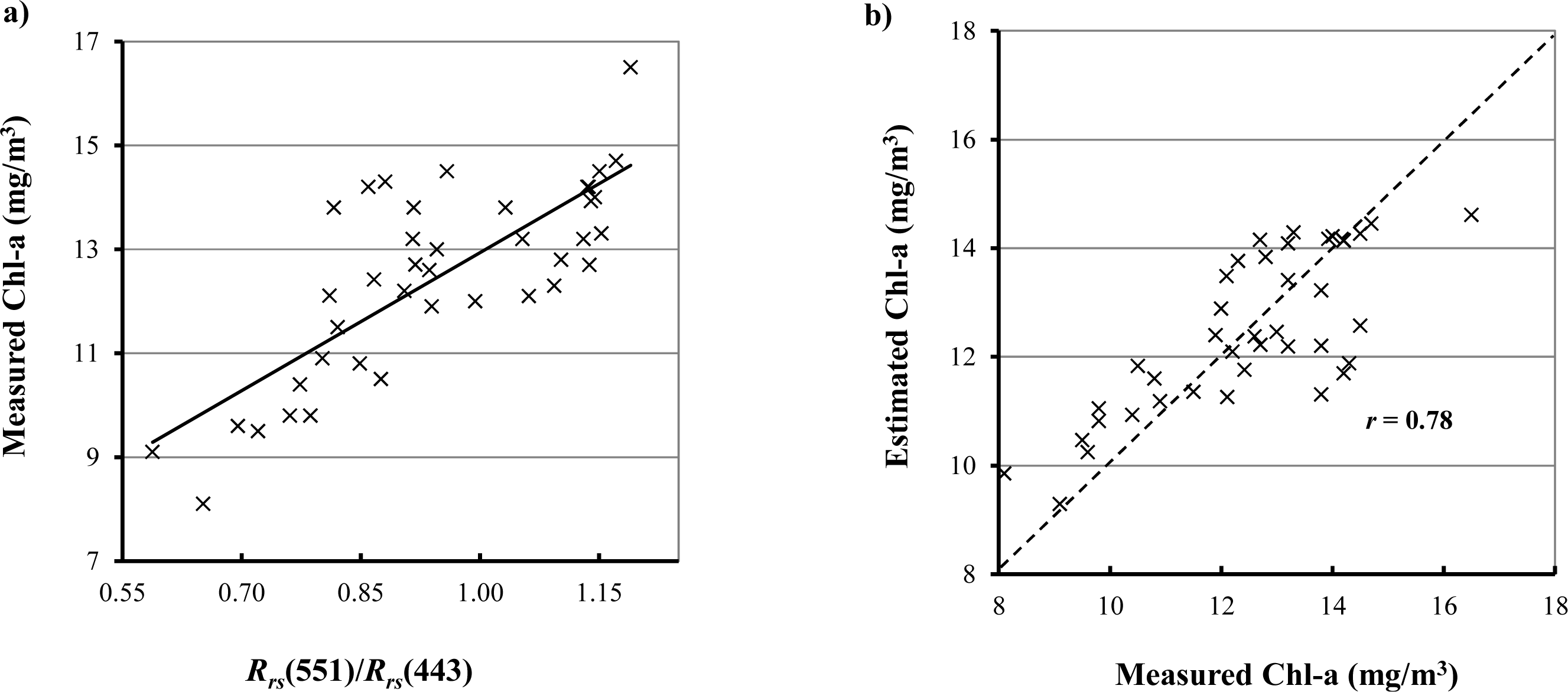
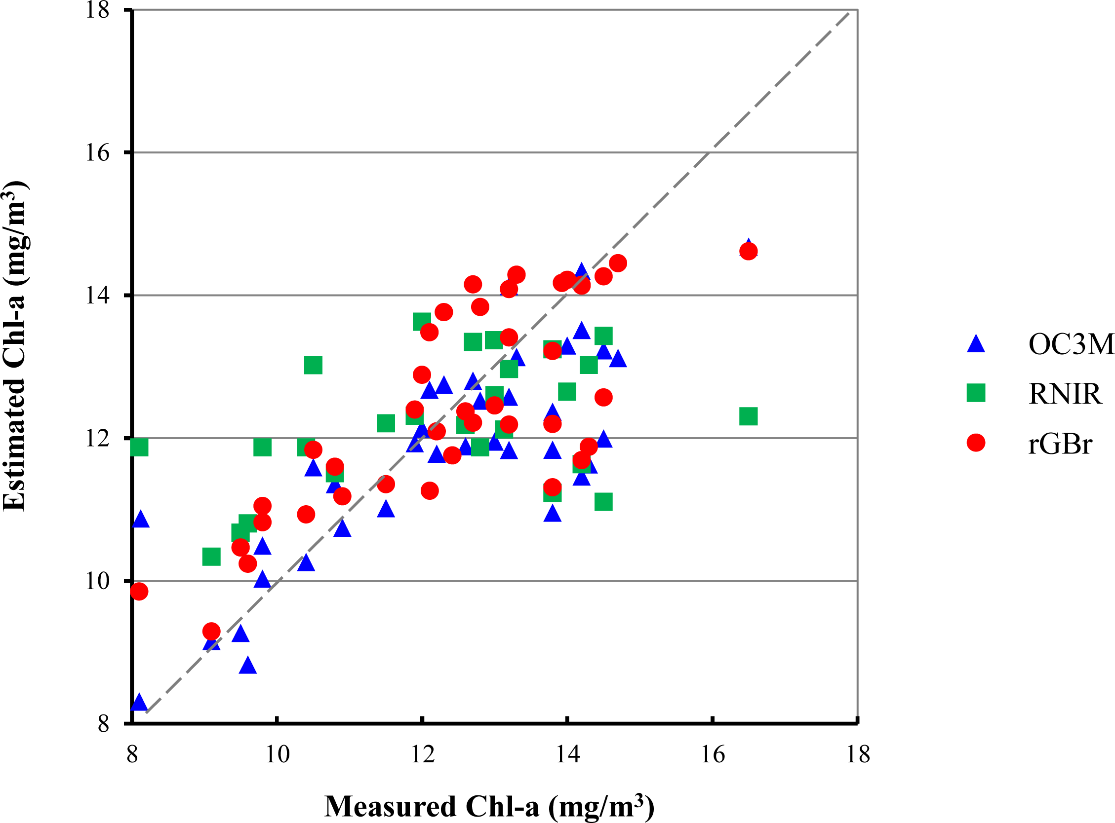
- Consideration of the optical properties of water shows that the concentration of Chl-a can be physically calculated by the ratio of the reflectances of the seawater surface at the visible green and blue wavelengths. The Chl-a concentrations in phytoplankton-rich coastal waters estimated by the proposed algorithm, rGBr, fit the measured in situ concentrations better and with smaller errors than the two previous representative algorithms, OC3M and RNIR.
- (3)
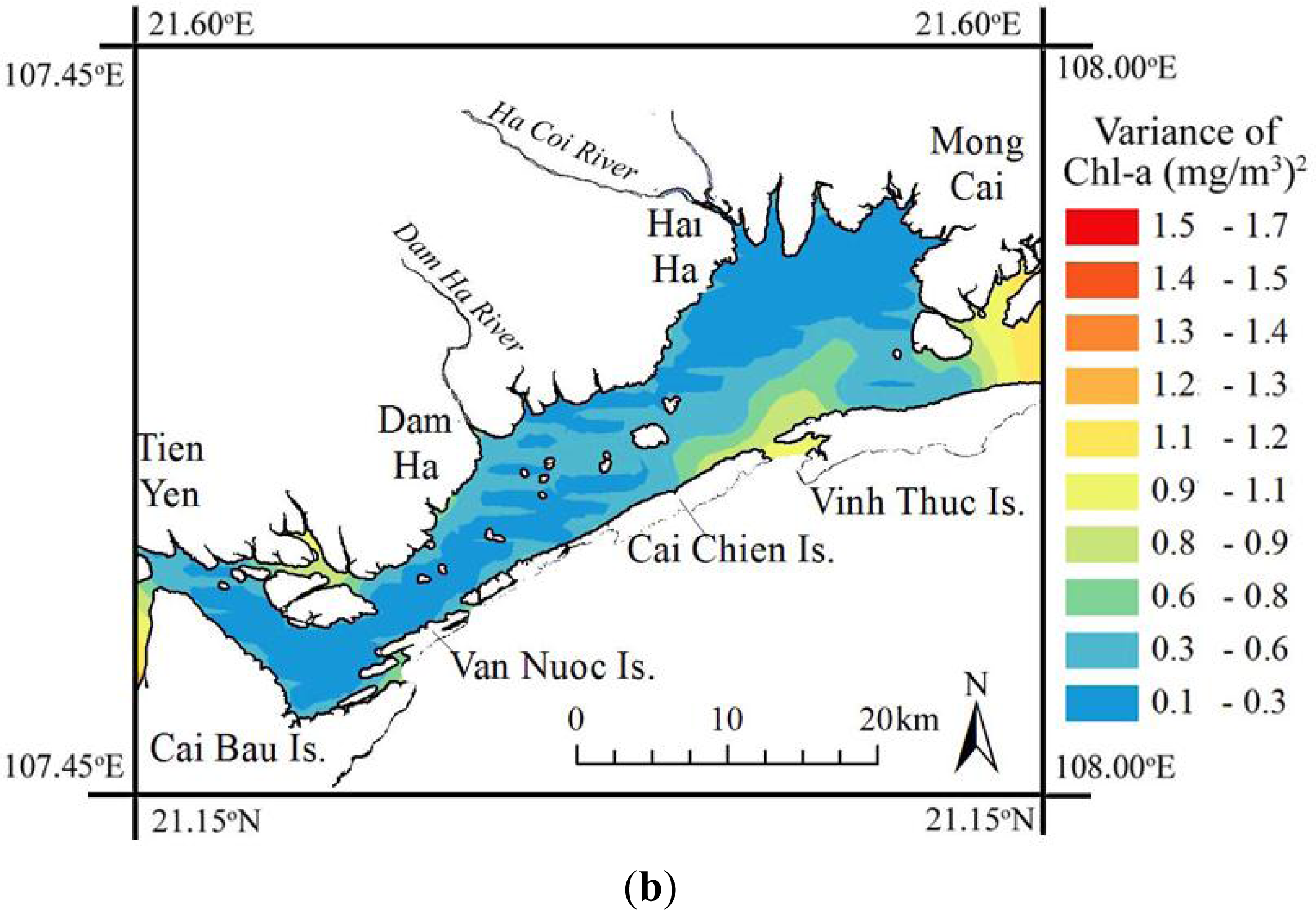
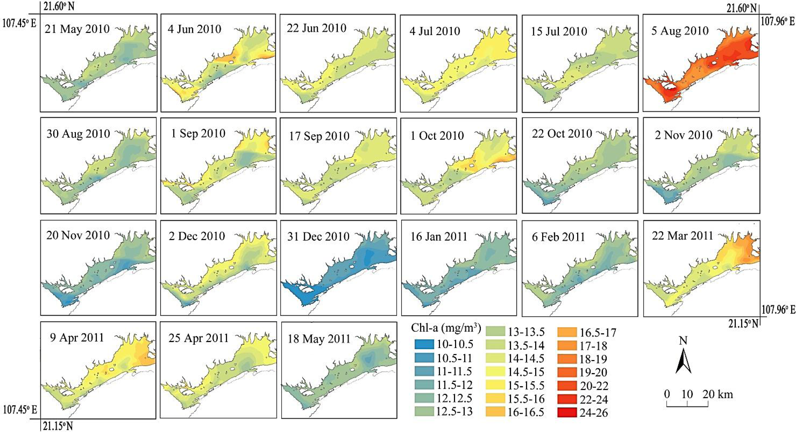
- The effectiveness of OK to improve the spatial resolution of the MODIS image-based estimation of Chl-a concentration from 1 km to 100 m was demonstrated. This improvement was possible because the OK map clarified the variation of Chl-a concentration in detail, particularly in local estuaries. From that OK map, the hydrodynamic system in Tien Yen Bay is suggested to be a main factor controlling the distribution of Chl-a concentrations.
- (4)
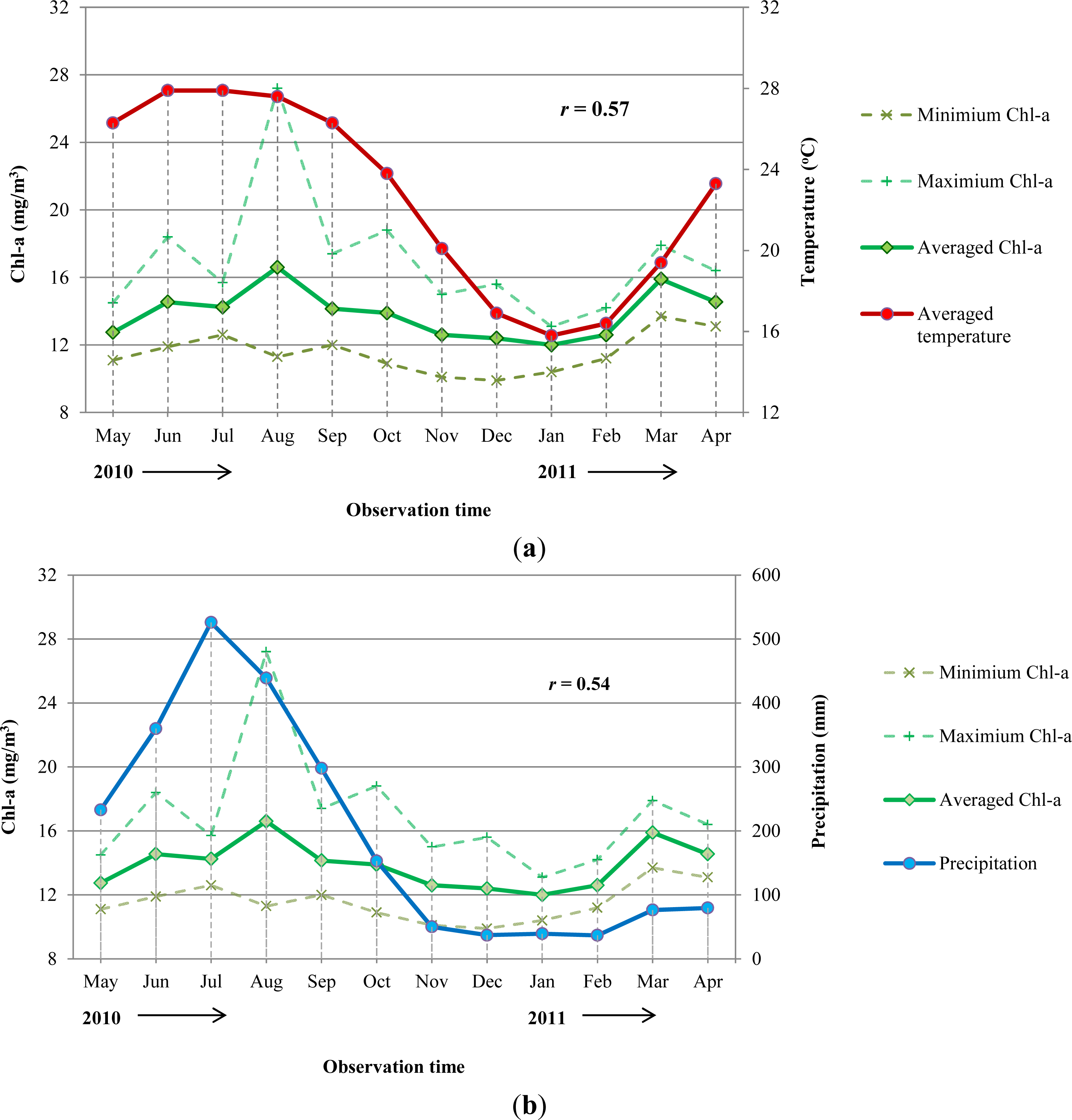
- By applying the rGBr and OK to the 21 scenes of MODIS image data from May 2010 to May 2011, notable features and seasonal trends were detected. In particular, the Chl-a concentrations have a bimodal variation. Furthermore, the waters of Tien Yen Bay can be labeled as naturally eutrophic, because of Chl-a values higher than 10 mg/m3 in the summer. This natural cause is supported by the correlation of Chl-a concentrations with representative meteorological factors, air temperature and precipitation.
Acknowledgments
Conflicts of Interest
References
- Matthews, A.M.; Duncan, A.G.; Davison, R.G. An assessment of validation techniques for estimating chlorophyll-a concentration from airborne multispectral imagery. Int. J. Remote Sens 2001, 22, 429–447. [Google Scholar]
- Cauwer, V.D.; Ruddick, K.; Park, Y.J.; Nechad, B.; Kyramarios, M. Optical remote sensing in support of eutrophication monitoring in the southern North Sea. EARSeL eProc 2004, 3, 208–221. [Google Scholar]
- Zimba, P.V.; Gitelson, A. Remote estimation of chlorophyll concentration in hyper-eutrophic aquatic systems: Model tuning and accuracy optimization. Aquaculture 2006, 256, 272–286. [Google Scholar]
- Schalles, J.F. Optical Remote Sensing Techniques to Estimate Phytoplankton Chlorophyll-a Concentrations in Coastal Waters with Varying Suspended Matter and CDOM Concentrations. In Remote Sensing of Aquatic Coastal Ecosystem Processes: Science and Management Application; Richardson, L.L., LeDew, E.F., Eds.; Springer: Dordrecht, The Netherlands, 2006; pp. 27–78. [Google Scholar]
- Ibrahim, A.N; Mabuchi, Y.; Murakami, M. Remote sensing algorithms for monitoring eutrophication in Ishizuchi storm water reservoir in Kochi Prefecture, Japan. Hydrol. Sci. J 2009, 50, 525–542. [Google Scholar]
- Gordon, H.R; Morel, A.Y. Remote Assessment of Ocean Color for Interpretation of Satellite Visible Imagery: A Review; Springer-Verlag: New York, NY, USA, 1983; pp. 1–114. [Google Scholar]
- Aiken, J.; Moore, G.F.; Trees, C.C.; Hooker, S.B.; Clark, D.K. The SeaWiFS CZCS-Type Pigment Algorithm. In SeaWiFS Technical Report Series; Hooker, S.B., Firestone, E.R., Eds.; NASA Goddard Space Flight Center: Greenbelt, MD, USA, 1995; Volume 29, pp. 1–34. [Google Scholar]
- O’Reilly, J.E.; Maritorena, S.; Mitchell, B.G.; Siegel, D.A.; Carder, K.L.; Garver, S.A.; Kahru, M.; McClain, C. Ocean color chlorophyll algorithms for SeaWiFS. J. Geophys. Res 1998, 103, 24937–24953. [Google Scholar]
- O’Reilly, J.E.; Maritorena, S.; Mitchell, B.G.; Siegel, D.A.; Carder, K.L.; Garver, S.A.; Kahru, M.; McClain, C. Ocean Color Chlorophyll a Algorithms for SeaWiFS, OC2, and OC4: Version 4. In SeaWiFS Postlaunch Technical Report Series, Volume 11, SeaWiFS Postlaunch Calibration and Validation Analyses, Part 3; Hooker, S.B., Firestone, E.R., Eds.; NASA Goddard Space Flight Center: Greenbelt, MD, USA, 2000; pp. 9–23. [Google Scholar]
- Carder, K.L.; Steward, R.G.; Harvey, G.R.; Ortner, P.B. Marine humic and fulvic acids: Their effects on remote sensing of ocean chlorophyll. Limnol. Oceanogr 1989, 34, 68–81. [Google Scholar]
- Gallegos, C.L.; Correll, D.L.; Pierce, J.W. Modeling spectral diffuse attenuation, absorption, and scattering coefficients in a turbid estuary. Limnol. Oceanogr 1990, 35, 1486–1502. [Google Scholar]
- Ritchie, J.C.; Schiebe, F.R.; Cooper, C.M.; Harrington, J.A., Jr. Chlorophyll measurements in the presence of suspended sediment using broad band spectral sensors aboard satellites. J. Freshwater Ecol 1994, 9, 197–206. [Google Scholar]
- Schalles, J.F.; Sheil, A.T.; Tycast, J.F.; Alberts, J.J.; Yacobi, Y.Z. Detection of Chlorophyll, Seston, and Dissolved Organic Matter in the Estuarine Mixing Zone of Georgia Coastal Plain Rivers. Proceedings of the Fifth International Conference on Remote Sensing for Marine and Coastal Environments, San Diego, CA, USA, 5–7 October 1998; pp. 315–324.
- Gons, H.J. Optical tele-detection of chlorophyll a in turbid inland waters. Environ. Sci. Technol 1999, 33, 1127–1132. [Google Scholar]
- Hladik, C.M. Close Range, Hyperspectral Remote Sensing of Southeastern Estuaries and an Evaluation of Phytoplankton Chlorophyll-a Predictive Algorithms. Creighton University, Omaha, NE, USA, 2004. [Google Scholar]
- Vertucci, F.A.; Likens, G.E. Spectral reflectance and water quality of Adirondack mountain region lakes. Limnol. Oceanogr 1989, 34, 1656–1672. [Google Scholar]
- Schalles, J.F.; Gitelson, A.A.; Yacobi, Y.Z.; Kroenke, A.E. Estimation of chlorophyll a from time series measurements of high spectral resolution reflectance in an eutrophic lake. J. Phycol 1998, 34, 383–390. [Google Scholar]
- Thiemann, S.; Kaufmann, H. Lake water quality monitoring using hyperspectral airborne data—A semiempirical multisensor and multitemporal approach for the Mecklenburg Lake District, Germany. Remote Sens. Environ 2002, 81, 228–237. [Google Scholar]
- Kallio, K.; Koponen, S.; Pulliainen, J. Feasibility of airborne imaging spectrometry for lake monitoring—A case study of spatial chlorophyll-a distribution in two meso-eutrophic lakes. Int. J. Remote Sens 2003, 24, 3771–3790. [Google Scholar]
- McGlathery, K.J.; Sundback, K.; Anderson, I.C. Eutrophication in shallow coastal bays and lagoons: the role of plants in coastal filter. Marine Ecol. Prog. Series 2007, 348, 1–18. [Google Scholar]
- Morel, A.; Prieur, L. Analysis of variations in ocean color. Limnol. Oceanogr 1977, 22, 709–722. [Google Scholar]
- Wu, M.; Zhang, W.; Wang, X.; Luo, D. Application of MODIS satellite data in monitoring water quality parameters of Chaohu Lake in China. Environ. Monit. Assess 2009, 148, 255–264. [Google Scholar]
- Vietnam Environment Protection Agency (VEPA), World Conservation Union (IUCN), Mekong Wetlands Biodiversity Conservation and Sustainable Use Programme (MWBP). Overview of Wetland Status in Vietnam following 15 Years of Ramsar Convention Implementation; VEPA: Hanoi, Vietnam, 2005; pp. 1–80. [Google Scholar]
- Hoang, V.T.; Pham, V.H. Biodiversity in Coastal Zones of Tien Yen—Dam Ha, Quang Ninh Province and Conservation. Proceeding of the 2nd Vietnam National Conference on Biodiversity (in Vietnamese), Hanoi, Vietnam, 17 October 2010; pp. 61–74.
- Thuoc, C.V. Phytoplankton in the Tien Yen, Bach Dang and Red River mouths. Marine Resour. Environ 1996, 3, 242–248. [Google Scholar]
- American Public Health Association (APHA). Standard Methods for the Examination of Water and Wastewater, 20th ed.; American Public Health Association: Washington, DC, USA, 1998; pp. E1–E15. [Google Scholar]
- Department of Environment, Climate Change and Water NSW. Waterwatch Estuary Field Mannual: A Manual for On-Site Use in the Monitoring of Water Quality and Estuary Health; Department of Environment, Climate Change and Water NSW: Sydney, Australia, 2010; pp. 2_6–2_7. [Google Scholar]
- Vietnam Ministry of Natural Resources and Environment. Vietnam Topographic Map; Scale 1/50,000; Department of Survey Map Publishing House: Hanoi, Vietnam, 2004. [Google Scholar]
- Chavez, J.P.S., Jr. An improved dark-object subtraction technique for atmospheric scattering correction of multispectral data. Remote Sens. Environ 1988, 24, 459–479. [Google Scholar]
- Bernstein, L.S.; Adler-Golden, S.M.; Sundberg, R.L.; Levine, R.Y.; Perkins, T.C.; Berk, A.; Ratkowski, A.J.; Felde, G.; Hoke, M.L. A New Method for Atmospheric Correction and Aerosol Optical Property Retrieval for VIS-SWIR Multi- and Hyperspectral Imaging Sensors: QUAC (QUick Atmospheric Correction). Proceedings of IEEE International Geosciences and Remote Sensing Symposium, Seoul, Korea, 25–27 July 2005; pp. 3549–3552.
- Hadjimitsis, D.G.; Clayton, C.R.I.; Hope, V.S. An assessment of the effectiveness of atmospheric correction algorithms through the remote sensing of some reservoirs. Int. J. Remote Sens 2004, 25, 3651–3674. [Google Scholar]
- Hadjimitsis, D.G.; Clayton, C.R.I. Field spectroscopy for assisting water quality monitoring and assessment in water treatment reservoirs using atmospheric corrected satellite remotely sensed imagery. Remote Sens 2011, 3, 362–377. [Google Scholar]
- Ha, N.T.T.; Koike, K. Integrating satellite imagery and geostatistics of point samples for monitoring spatio-temporal changes of total suspended solids in bay waters: application to Tien Yen Bay (Northern Vietnam). Frontiers Earth Sci 2011, 5, 305–316. [Google Scholar]
- Moses, W.J.; Gitelson, A.A.; Berdnikov, S.; Povazhnyy, V. Estimation of chlorophyll-a concentration in case II waters using MODIS and MERIS data-successes and challenges. Environ. Res. Lett 2009, 4. [Google Scholar] [CrossRef]
- Carder, K.L.; Chen, F.R.; Cannizzaro, J.P.; Campbell, J.W.; Mitchell, B.G. Performance of the MODIS semi-analytical ocean color algorithm for chlorophyll-a. Adv. Space Res 2004, 33, 1152–1159. [Google Scholar]
- Gitelson, A. The Peak near 700 nm on Radiance Spectra of algae and water - Relationships of its magnitude and position with chlorophyll concentration. Int. J. Remote Sens 1992, 13, 3367–3373. [Google Scholar]
- Antoite, D.; Andre, J.M.; Morel, A. Oceanic primary production 2: Estimation of global scale from satellite (coastal zone color scanner) chlorophyll. Glob. Biogeochem. Cy 1996, 10, 57–69. [Google Scholar]
- D’Sa, E.J.; Miller, R.L. Bio-optical properties in waters influenced by the Mississippi River during low flow conditions. Remote Sens. Environ 2002, 84, 538–549. [Google Scholar]
- Dall’Olmo, G.; Gitelson, A.A.; Rundquist, D.C. Toward a unified approach for remote estimation of chlorophyll-a in both terrestrial vegetation and turbid productive waters. Geophys. Res. Lett 2003, 30, 1938–1941. [Google Scholar]
- Gilerson, A.A; Gitelson, A.A.; Zhou, J.; Gurlin, D.; Moses, W.; Ioannou, I.; Ahmed, S. Algorithms for remote estimation of chlorophyll-a in coastal and inland waters using red and near infrared bands. Opt. Express 2010, 18, 24109–24125. [Google Scholar]
- Lee, Z.P.; Carder, K.L.; Hawes, S.H.; Steward, R.G.; Peacock, T.G.; Davis, C.O. A model for interpretation of hyperspectral remote-sensing reflectance. Appl. Opt 1994, 33, 5721–5732. [Google Scholar]
- Gordon, H.R.; Brown, O.B.; Jacobs, M.M. Computed relationships between the inherent and apparent optical properties of a flat homogeneous ocean. Appl. Opt 1975, 14, 417–427. [Google Scholar]
- Jerome, J.H.; Bukata, R.P.; Burton, J.E. Utilizing the components of vector irradiance to estimate the scalar irradiance in natural waters. Appl. Opt 1988, 27, 4012–4018. [Google Scholar]
- Kirk, J.T.O. Volume scattering function, average cosines, and the underwater light field. Limnol. Oceanogr 1991, 36, 455–467. [Google Scholar]
- Barnard, A.H.; Ronald, J.; Zaneveld, V.; Pegau, S.W. In situ determination of the remotely sensed reflectance and the absorption coefficient: Closure and inversion. Appl. Opt 1999, 38, 5108–5117. [Google Scholar]
- Carder, K.L.; Chen, F.R.; Lee, Z.; Hawes, S.K.; Cannizzaro, J.P. Case 2 Chlorophyll a. In MODIS Ocean Science Team Algorithm Theoretical Basis Document; Version 7; NASA Goddard Space Flight Center: Greenbelt, MD, USA, 2003; pp. 4–67. [Google Scholar]
- Morel, A. Optical Properties of Pure Water and Pure Seawater. In Optical Aspects of Oceanography; Jerlov, N.G., Nielson, E.S., Eds.; Academic Press: London, UK, 1974; pp. 1–24. [Google Scholar]
- Smith, R.C.; Baker, K.S. Optical properties of the clearest natural waters (200–800 nm). Appl. Opt 1981, 20, 177–184. [Google Scholar]
- Twardowski, M.S.; Claustre, H.; Freeman, S.A.; Stramski, D.; Huot, Y. Optical backscattering properties of the “clearest” natural waters. Biogeosciences 2007, 4, 1041–1058. [Google Scholar]
- McKee, D.; Cunningham, A.; Slater, J.; Jones, K.J.; Griffiths, C.R. Inherent and apparent optical properties in coastal waters: A study of the Clyde Sea in early summer. Estuar. Coast. Shelf Sci 2002, 56, 369–376. [Google Scholar]
- McKee, D.; Cunningham, A. Identification and characterisation of two optical water types in the Irish Sea from in situ inherent optical properties and seawater constituents. Estuar. Coast. Shelf Sci 2006, 68, 305–316. [Google Scholar]
- Whitmire, A.L.; Boss, E.; Cowles, T.J.; Pegau, W.S. Spectral variability of the particulate backscattering ratio. Opt. Expr 2007, 15, 7019–7031. [Google Scholar]
- Park, Y.J; Ruddick, K. Model of remote-sensing reflectance including bidirectional effects for case 1 and case 2 waters. Appl. Opt 2005, 44, 1236–1249. [Google Scholar]
- Babin, M.; Stramski, D.; Ferrari, G.M.; Claustre, H.; Bricaud, A.; Obolensky, G.; Hoepffner, N. Variations in the light absorption coefficients of phytoplankton, non-algal particles, and dissolved organic matter in coastal waters around Europe. J. Geophys. Res 2003, 108, 4_1–4_20. [Google Scholar]
- Fishwick, J.R.; Aiken, J.; Barlow, R.G.; Sessions, H.; Bernard, S.; Ras, J. Functional relationships and bio-optical properties derived from phytoplankton pigments, optical and photosynthetic parameters; a case study of the Benguela ecosystem. J. Mar. Biol. Assoc. UK 2006, 86, 1267–1280. [Google Scholar]
- Hirata, T.; Aiken, J.; Hardman-Mountford, N.; Smyth, T.J.; Barlow, R.G. An absorption model to determine phytoplankton size classes from satellite ocean colour. Remote Sens. Environ 2009, 112, 3153–3159. [Google Scholar]
- Carder, K.L.; Cannizzaro, J.P.; Lee, Z. Ocean color algorithms in optically shallow waters: Limitation and improvements. Proc. SPIE 2005, 5885. [Google Scholar] [CrossRef]
- Cannizzaro, J.P.; Carder, K.L. Estimating chlorophyll a concentration from remote-sensing reflectance in optically shallow waters. Remote Sens. Environ 2006, 101, 13–24. [Google Scholar]
- Aiken, J.; Pradhan, Y.; Barlow, R.G.; Lavender, S.; Poulton, A.; Holligan, P.M.; Hardman-Mountford, N. Phytoplankton pigments and functional types in the Atlantic Ocean: A decadal assessment, 1995–2005. Deep-Sea Res. Part II: Top. Stud. Oceanogr 2009, 56, 899–917. [Google Scholar]
- Cressie, N.A.C. Statistics for Spatial Data; John Wiley & Sons, Inc: New York, NY, USA, 1993; pp. 1–900. [Google Scholar]
- Kanaroglou, P.S.; Soulakellis, N.A.; Sifakis, N.I. Improvement of satellite derived pollution maps with the use of a geostatistical interpolation method. J. Geogr. Syst 2001, 4, 193–208. [Google Scholar]
- Zhang, C.; Li, W.; Travis, D. Restoration of clouded pixels in multispectral remotely sensed imagery with co-kriging. Int. J. Remote Sens 2009, 30, 2173–2195. [Google Scholar]
- Meng, Q.; Borders, B.; Madden, M. High-resolution satellite image fusion using regression kriging. Int. J. Remote Sens 2010, 31, 1857–1876. [Google Scholar]
- Petrie, G.M.; Heasler, P.G.; Perry, E.M.; Thompson, S.E.; Daly, D.S. Inverse kriging to enhance spatial resolution of imagery. Proc. SPIE 2002, 4789. [Google Scholar] [CrossRef]
- Wang, X.J.; Liu, R.M. Spatial analysis and eutrophication assessment for chlorophyll a in Taihu Lake. Environ. Monit. Assess 2005, 101, 167–74. [Google Scholar]
- Müller, D. Estimation of Algae Concentration in Cloud Covered Scenes Using Geostatistical Methods. Proceeding of ENVISAT Symposium 2007, Montreux, Switzerland, 23–27 April 2007.
- Georgakarakos, S.; Kitsiou, D. Mapping abundance distribution of small pelagic species applying hydroacoustics and Co-Kriging techniques. Hydrobiologia 2008, 612, 155–169. [Google Scholar]
- Saulquin, B.; Gohin, F.; Garrello, R. Regional objective analysis for merging high-resolution MERIS, MODIS/Aqua, and SeaWiFS Chlorophyll-a data from 1998 to 2008 on the European Atlantic Shelf. IEEE Trans. Geosci. Remote Sens 2010, 49, 143–154. [Google Scholar]
- Shehhi, M.R.A.; Gherboudj, I.; Estima, J.; Ghedira, H. Geospatial Analysis of the Red-Tide over the Arabian Gulf. Proceeding of the 1st Geospatial Scientific Summit, Dubai, United Arab Emirates, 12–13 November 2012.
- Agrawal, G.; Sarup, J. Comparision of QUAC and FLAASH atmospheric correction modules on EO-1 Hyperion data of Sanchi. Int. J. Adv. Eng. Sci. Technol 2011, 4, 178–186. [Google Scholar]
- Simboura, N.; Panayotidis, P.; Papathanassiou, E. A synthesis of the biological quality elements for the implementation of the European Water Framework Directive in the Mediterranean ecoregion: The case of Saronikos Gulf. Ecol. Indic 2005, 5, 253–266. [Google Scholar]
- Morton, B.; Blackmore, G. South China Sea. Mar. Pollut. Bull 2001, 42, 1236–1263. [Google Scholar]
- Quangninh Province Statistics Office. Quangninh. Statistical Yearbook 1955–2011; Statistical Publishing House: Hanoi, Vietnam, 2012; pp. 1–548. [Google Scholar]
- Lihan, T.; Mustapha, M.A.; Rahim, S.A.; Saitoh, S.; Iida, K. Influence of river plume on variability of chlorophyll a concentration using satellite images. J. Appl. Sci 2011, 11, 484–493. [Google Scholar]
- CSTT (Comprehensive Study Task Team of Group Coordinating Sea Disposal Monitoring). Comprehensive Studies for the Purposes of Article 6 & 8.5 of DIR 91/271 EEC, the Urban. Waste Water Treatment Directive, 2nd ed.; The Scottish Environment Protection Agency and Water Service Association: Edinburgh, UK, 1997; pp. 8–11. [Google Scholar]
- Cannizzaroa, J.P.; Cardera, K.L.; Chena, F.R.; Heilb, C.A.; Vargoa, G.A. A novel technique for detection of the toxic dinoflagellate, Kareniabrevis, in the Gulf of Mexico from remotely sensed ocean color data. Cont. Shelf Res 2008, 28, 137–158. [Google Scholar]


| Data Obtained from DOS for Bands | Data Obtained from QUAC for Bands | |||||||||
|---|---|---|---|---|---|---|---|---|---|---|
| 9 | 10 | 12 | 13 | 15 | 9 | 10 | 12 | 13 | 15 | |
| Average | 0.043 | 0.040 | 0.042 | 0.022 | 0.036 | 0.117 | 0.039 | NaN | NaN | NaN |
| Maximum | 0.077 | 0.082 | 0.090 | 0.036 | 0.010 | 0.147 | 0.072 | NaN | NaN | NaN |
| Minimum | 0.026 | 0.021 | 0.015 | 0.010 | 0.024 | 0.065 | 0.039 | NaN | NaN | NaN |
| Out of 40 pixels | 0 | 0 | 0 | 13 | 8 | 0 | 0 | 40 | 40 | 40 |
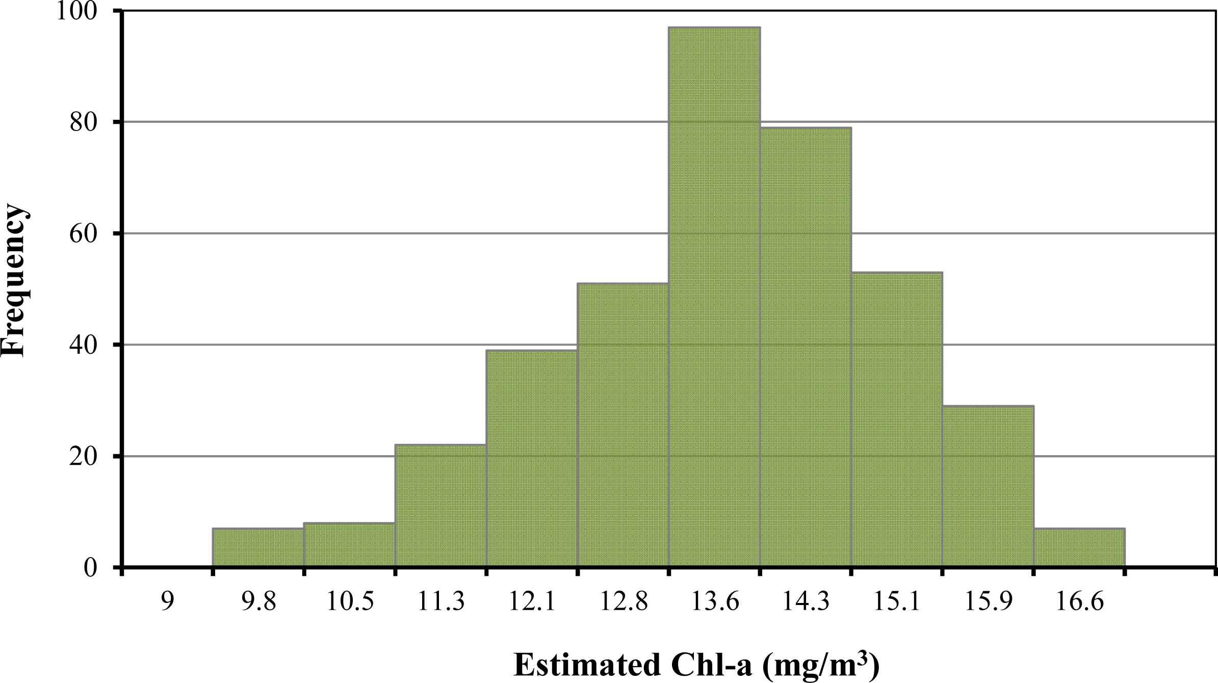
| Sample Data | Estimation from MODIS | Prediction by OK | |
|---|---|---|---|
| Number of data | 40 | 392 | 392 |
| Mean | 12.5 | 13.3 | 13.3 |
| Median | 12.7 | 13.3 | 13.3 |
| Maximum | 16.5 | 16.6 | 16.1 |
| Minimum | 8.1 | 9.0 | 9.9 |
| Standard deviation | 1.8 | 1.4 | 1.3 |
| Range | 8.4 | 7.6 | 6.3 |
| Algorithm | Models with Empirical Coefficients | r | MSE (mg/m3) | RMSE (mg/m3) | ||
|---|---|---|---|---|---|---|
| Average | Max | Min | ||||
| OC3M (O’Reilly et al., 2000) | 0.65 | 1.19 | 5.48 | 0.03 | 1.70 | |
| RNIR (Gilerson et al., 2010) | 0.43 | 1.48 | 4.19 | 0.23 | 1.82 | |
| rGBr | 0.78 | 0.90 | 2.51 | 0.05 | 1.13 | |
© 2014 by the authors; licensee MDPI, Basel, Switzerland This article is an open access article distributed under the terms and conditions of the Creative Commons Attribution license ( http://creativecommons.org/licenses/by/3.0/).
Share and Cite
Ha, N.T.T.; Koike, K.; Nhuan, M.T. Improved Accuracy of Chlorophyll-a Concentration Estimates from MODIS Imagery Using a Two-Band Ratio Algorithm and Geostatistics: As Applied to the Monitoring of Eutrophication Processes over Tien Yen Bay (Northern Vietnam). Remote Sens. 2014, 6, 421-442. https://doi.org/10.3390/rs6010421
Ha NTT, Koike K, Nhuan MT. Improved Accuracy of Chlorophyll-a Concentration Estimates from MODIS Imagery Using a Two-Band Ratio Algorithm and Geostatistics: As Applied to the Monitoring of Eutrophication Processes over Tien Yen Bay (Northern Vietnam). Remote Sensing. 2014; 6(1):421-442. https://doi.org/10.3390/rs6010421
Chicago/Turabian StyleHa, Nguyen Thi Thu, Katsuaki Koike, and Mai Trong Nhuan. 2014. "Improved Accuracy of Chlorophyll-a Concentration Estimates from MODIS Imagery Using a Two-Band Ratio Algorithm and Geostatistics: As Applied to the Monitoring of Eutrophication Processes over Tien Yen Bay (Northern Vietnam)" Remote Sensing 6, no. 1: 421-442. https://doi.org/10.3390/rs6010421