Karst Depression Detection Using ASTER, ALOS/PRISM and SRTM-Derived Digital Elevation Models in the Bambuí Group, Brazil

Abstract

Remote sensing has been used in karst studies to identify limestone terrain, describe exokarst features, analyze karst depressions, and detect geological structures important to karst development. The aim of this work is to investigate the use of ASTER-, SRTM- and ALOS/PRISM-derived digital elevation models (DEMs) to detect and quantify natural karst depressions along the São Francisco River near Barreiras city, northeast Brazil. The study area is a karst landscape characterized by karst depressions (dolines), closed depressions in limestone, many of which contain standing water connected with the ground-water table. The base of dolines is typically sealed with an impermeable clay layer covered by standing water or herbaceous vegetation. We identify dolines by combining the extraction of sink depth from DEMs, morphometric analysis using GIS, and visual interpretation. Our methodology is a semi-automatic approach involving several steps: (a) DEM acquisition; (b) sink-depth calculation using the difference between the raw DEM and the corresponding DEM with sinks filled; and (c) elimination of falsely identified karst depressions using morphometric attributes. The advantages and limitations of the applied methodology using different DEMs are examined by comparison with a sinkhole map generated from traditional geomorphological investigations based on visual interpretation of the high-resolution remote sensing images and field surveys. The threshold values of the depth, area size and circularity index appropriate for distinguishing dolines were identified from the maximum overall accuracy obtained by comparison with a true doline map. Our results indicate that the best performance of the proposed methodology for meso-scale karst feature detection was using ALOS/PRISM data with a threshold depth > 2 m; areas > 13,125 m² and circularity indexes > 0.3 (overall accuracy of 0.53). The overall correct identification of around half of the true dolines suggests the potential to substantially improve doline identification using higher-resolution LiDAR-generated DEMs.

1. Introduction

Karst depressions cause damage both in rural areas through the loss of arable land and in urban areas due to damage to buildings, roads, and water supply systems [1,2]. Problems caused by karst depressions have motivated many studies on their identification and spatial distribution using remote sensing data [3,4]. Historical changes and variations in the number and shape of karst depressions can be obtained from comparative studies of multitemporal images [5,6].

Remote sensing also allows inferences about subsurface karst structures (endokarst). The regularity of the patterns and surface alignments of karst features often are associated with joint patterns, faulting and folding. Conduits in karst groundwater are formed from rock dissolution along planes or discontinuities where the flow has characteristics similar to the water surface [7,8]. Endokarst environments are typically characterized by open conduits with low capacity for storage and rapid groundwater flow. This intimate relationship between surface water and groundwater defines a system of interconnected caves and superficial features. Due to such relationships, the locations of karst aquifers or preferential flowpaths for groundwater have been inferred by the positions of fracture sets or doline alignments apparent on aerial photographs and satellite images [9–11]. In addition, remote-sensing data are used as inputs in GIS models for detecting and monitoring areas vulnerable to groundwater pollution in karst terrain [12,13].

Digital terrain data are widely used to describe surface features and quantify topographic characteristics [14–17] and morphometric attributes derived from Digital Elevation Models (DEMs) have been used for automatic detection of elemental forms associated with landforms [18–20]. Several studies employ terrain attributes to characterize and describe karst processes [21–23]. In karst-depression detection studies a promising terrain attribute is the sink depth derived from the depression-filling algorithm [24–27]. Such algorithms are an integral component of spatially distributed hydrological models that delineate watersheds, drainage networks and overland flowpaths [28–32]. Other methods to automate karst depression recognition include convolution or filtering with kernel windows using focal functions [33] and the “active-contour” method [34,35], an algorithm that delineates sinkhole boundaries with a compactness test and by fitting a local bi-quadratic surface to the points surrounding the potential sinkhole locations. However, tests made with ASTER (Advanced Spaceborne Thermal Emission and Reflection Radiometer) and SRTM (Shuttle Radar Topography Mission) [25,26] DEM data have shown that these data are not sufficient for karst depression detection, making it necessary to combine the above approach with other methods to automate and improve the process of depression mapping. For example, Guimarães et al. [25] combined this approach with digital classification of spectral images and Siart et al. [26] used an iron-oxide ratio and the vegetation infrared/red ratio from Quickbird imagery. The increasing availability of high-resolution DEMs and satellite images promises improved detection of karst depressions through the combination of DEM analysis and remote sensing.

The present paper aims to develop a semi-automatic method for doline identification in central Brazil using three different DEMs: (a) the ASTER Global Digital Elevation Model (ASTER-GDEM) Version 1 from the USA’s National Aeronautics and Space Administration (NASA) and Japan’s Ministry of Economy, Trade and Industry (METI); (b) the SRTM Version 4.1 DEM compiled by the Consultative Group on International Agricultural Research Consortium for Spatial Information (CGIAR-CSI); and (c) the DEM made from the high-resolution satellite sensor Advanced Land Observing Satellite/Panchromatic Remote-sensing Instrument for Stereo Mapping (ALOS/PRISM).

The approach combines a threshold sink depth and morphometric analysis in order to refine the identification of karst depressions. Here, our focus is limited to automated DEM-based classification and we do not address the strong potential for improved identification of dolines by combining DEM analysis with image classification [22,23]. We compare performance among sensors to evaluate the efficiency of each data type for use in automated sinkhole mapping and use traditional geomorphological methods of field surveys and visual image interpretation to assess the advantages and limitations of the automated technique.

2. Study Area

Brazil has 425,000–600,000 km² of limestone rocks in different biomes [35] and knowledge of karst areas has been reinforced by speleological studies and investigations of biological, paleoenvironmental, paleontological, and archaeological attributes. Karmann & Sánchez’s [36] classified speleological provinces in Brazil based on common geological history, stratigraphic associations with carbonate and pelitic sequences, and thickness and extension of carbonate rocks.

We analyzed a small area of the Bambuí Speleological Province in Central Brazil. This province is underlain by rocks of the Bambuí Group [37], a Neoproterozoic sedimentary sequence that records at least two transgressive-regressive cycles in the epicontinental basin and possibly deposition in a foreland basin along the west side of the São Francisco Craton during the Brasiliano orogeny [38–41]. 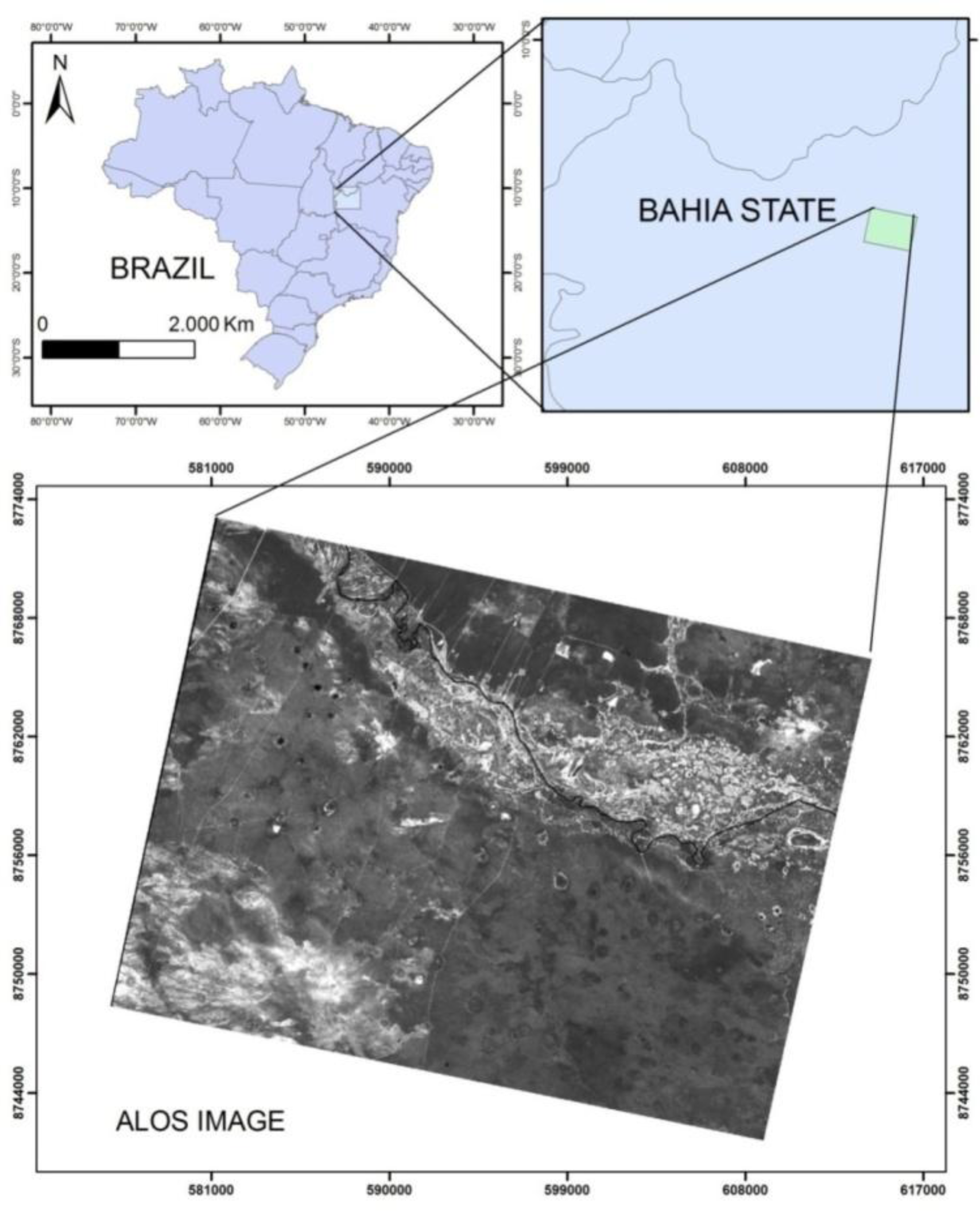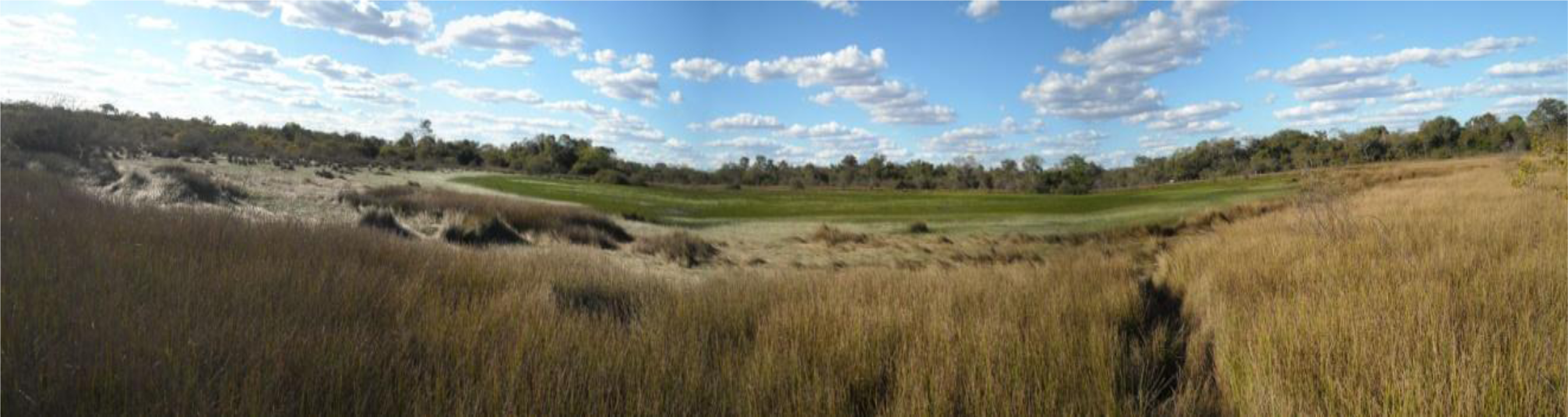The study area is located in Bahia State, northeastern Brazil (Figure 1) where the tropical environment favors karst formation due to the growth of vegetation and biochemical activity increasing water acidity and promoting the development of vertical flow and sinkhole (doline) development. The study area has a high density of dolines associated with the exposure of karstified limestone. The stagnant surface water and shallow groundwater mostly reside in the sinks, forming lakes. Herbaceous vegetation dominates in topographic depressions because trees have low tolerance to shallow groundwater. Thus, dolines commonly are floored by open water or herbaceous vegetation (Figure 2). The vegetation cover in the study area therefore has little potential influence on the results from different sensor types, unlike other areas with forest.

3. Material and Methods

We compared three different DEMs—ASTER-GDEM, ALOS/PRISM-DEM and SRTM-DEM—all processed in four steps, the first of which was DEM acquisition and evaluation of the best DEM for our purposes. We next identified closed depressions or sinks in the DEMs and digitally “filled” them by interpolation from neighboring elevations outside the depression polygons. We calculated sink depths as the difference between the original and processed DEMs. The final step was the elimination of false detections using morphometric attributes and visual interpretation overlaying the depression vectors on the high-resolution remotely sensed image.

3.1. Digital Elevation Model

We analyzed the potential of DEMs for mapping closed depressions using data from different sensors with various data-acquisition methods and spatial resolution: ASTER-GDEM (30 m), ALOS/PRISM-DEM (5 m) and SRTM-DEM (90 m).

The ASTER-GDEM was generated using ASTER Level-1A bands 3N (nadir-viewing) and 3B (backward-viewing) images from the Visible/Near-Infrared (VNIR) sensor. The VNIR subsystem consists of nadir- and rear-viewing telescopes looking 0° and 27.7° backwards that allow the generation of stereoscopic data with a time lag around one minute [42]. The Band-3 stereo pair is acquired in the spectral range of 0.78–0.86 μm with a base-to-height ratio of 0.6. In 2006, LP DAAC implemented software based on an automated stereo-correlation method that utilizes the ephemeris and attitude data derived from both the ASTER instrument and the Terra spacecraft platform. This method generates a relative DEM without any ground control points (GCPs). The ASTER-GDEM is an image product with a horizontal resolution of 1 arc-second (30 m) referenced to the UTM coordinate system, and referenced to Earth’s geoid using the EGM96 geopotential model. This product is generated from a stereo-pair of images using the SilcAST software and covers the earth’s surface between 83°N and 83°S, encompassing 99 percent of Earth’s landmass.

The SRTM flown on Space Shuttle Endeavour in February 2,000 carried in the cargo bay two synthetic aperture radars, a C-band system (5.6 cm; C-RADAR) and an X-band system (3.1 cm; X-RADAR) [43]. Radar data are less sensitive to cloud cover than optical data. Topographic data were acquired from a single flight covering 80% of Earth's land surface in just 11 days, between the latitudes 60°N and 57°S. The flyover produced three-dimensional models with spatial resolutions of 1 arc sec (30 m) and 3 arc sec (90 m) using WGS84 horizontal datum and vertical datum WGS84/EGM96. Vertical accuracy was on the order of 5 m [44]. The continuous data acquisition (i.e., day and night regardless of clouds, which are transparent to the RADAR) ensured homogeneous data throughout the globe, making the SRTM-DEM an important tool for studies of the land surface [44–46]. SRTM-DEM data have been widely used for geomorphological studies [47,48].

The ALOS was launched on 24 January 2006 by the Japan Aerospace Exploration Agency (JAXA) with PRISM on board, which acquires images with spatial resolution of 2.5 m. PRISM produces triplet images that achieve along-track stereoscopy by three independent cameras for viewing nadir, forward and backward where the images are acquired in the same orbit at almost the same time [41,49]. The nadir-looking radiometer can provide coverage 70 km wide, and the forward-looking and backward-looking radiometers each provide coverage 35 km wide [50]. Several studies assess the absolute vertical accuracy (relationship between DEM elevation and true elevation relative to an established vertical datum) of the ALOS/PRISM-DEM. Gruen et al. [51] compared the DEM accuracy of ALOS/PRISM data with other satellite or ground control points and found that its accuracy is similar to that obtained by SPOT 5, IKONOS and QuickBird data. Kocaman and Gruen [52] also found similar results for IKONOS, but reported a lower accuracy compared to SPOT-5 results. Maruya and Ohyama [49] used ground control points derived from the 1:25,000 mapping to analyze elevation accuracy and found a 6.2 m mean error and a 4.8 m RMSE. Saunier et al. [53] verified that the accuracy in height for the ALOS/PRISM-DEM is about 1 m using either five or nine ground control points. In Brazil ALOS/PRISM-DEM was tested in an area with steep slopes and comparison of the results to ground control points (GCP), indicated an accuracy comparable to 1:25,000 scale mapping [54]. Although the studies described above address the absolute vertical accuracy, for this study the relative vertical accuracy is most important and is obtained from a vertical difference between two points, i.e., a measure of the point-to-point vertical accuracy within a specific dataset. The absolute vertical error is greater than the relative vertical error, establishing an upper limit for empirical evaluation of relative vertical accuracy.

The stereo DEM extraction from ALOS/PRISM data was done using the commercial software, PCI Geomatica orthoengine. Artifacts in the data were assessed by visual inspection and specific algorithms [55,56] that reveal errors on the image border and in areas with cloud cover. Image-border errors were eliminated from the image during resizing by simply removing the noisy strip. The cloud cover is a limitation of this type of data and anomalous values are easily identified by digital processing from a threshold value and thus can be identified and discarded. The scenes used in this study have few and isolated clouds.

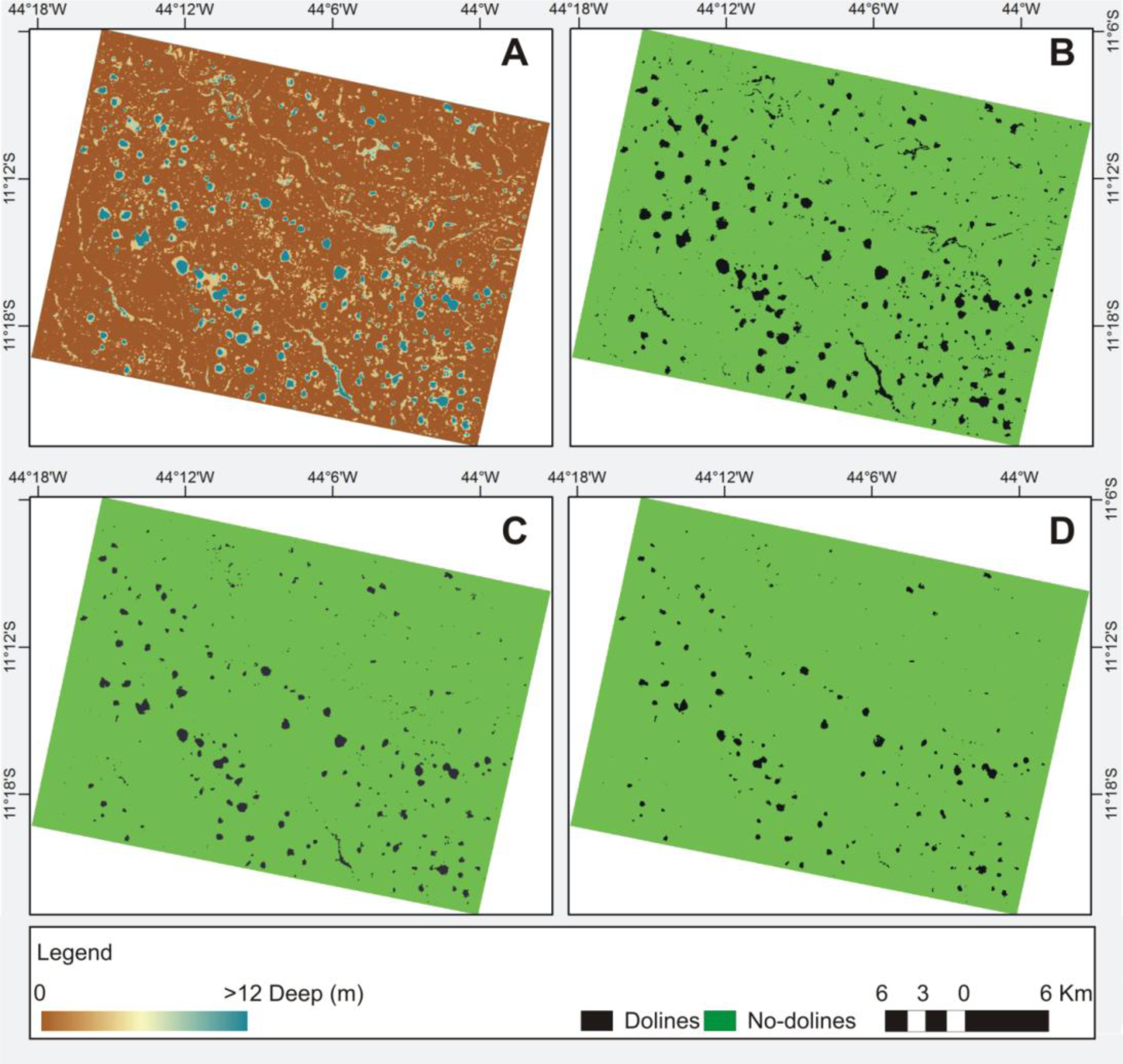
3.2. Sink-Depth Image

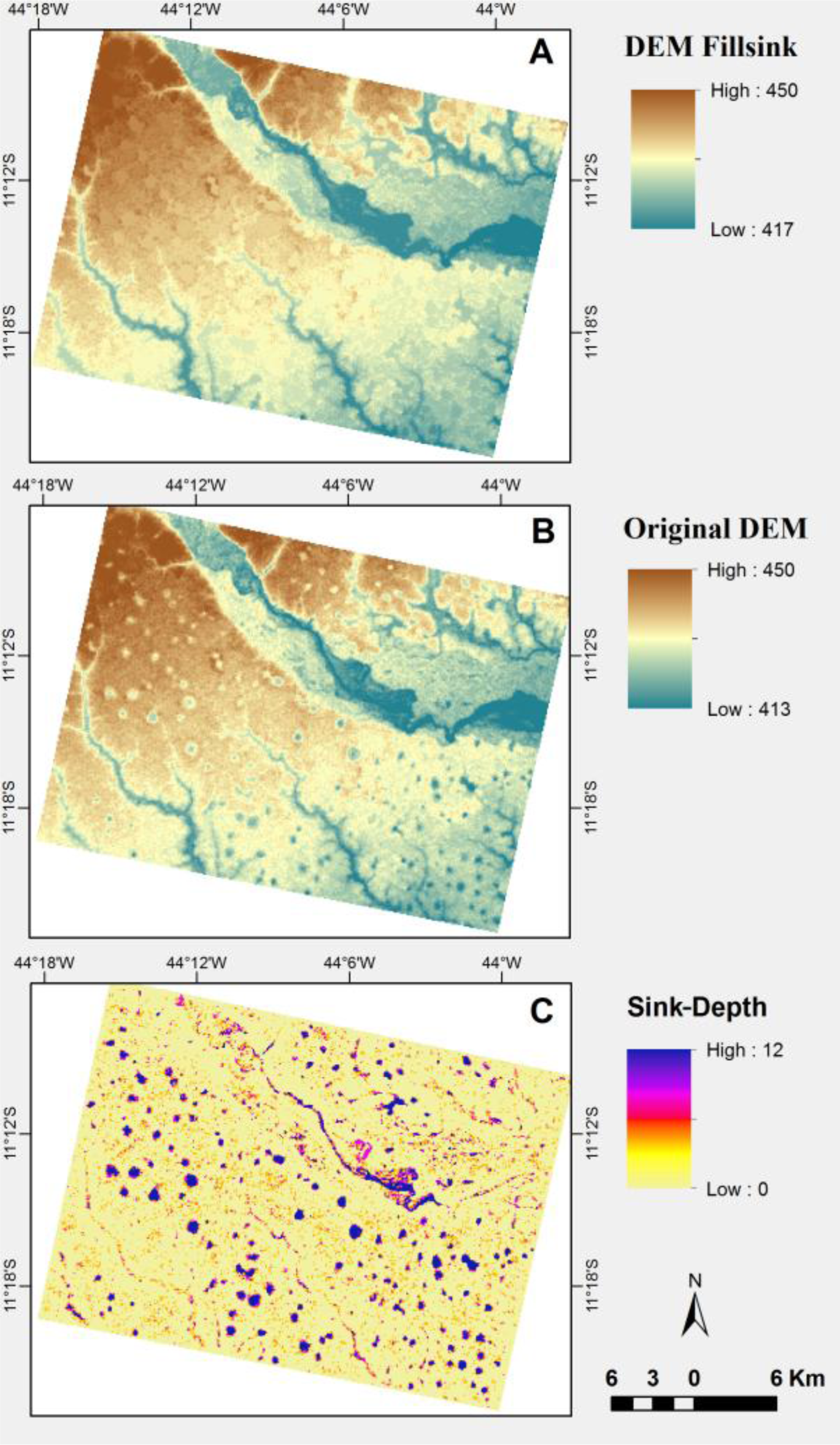
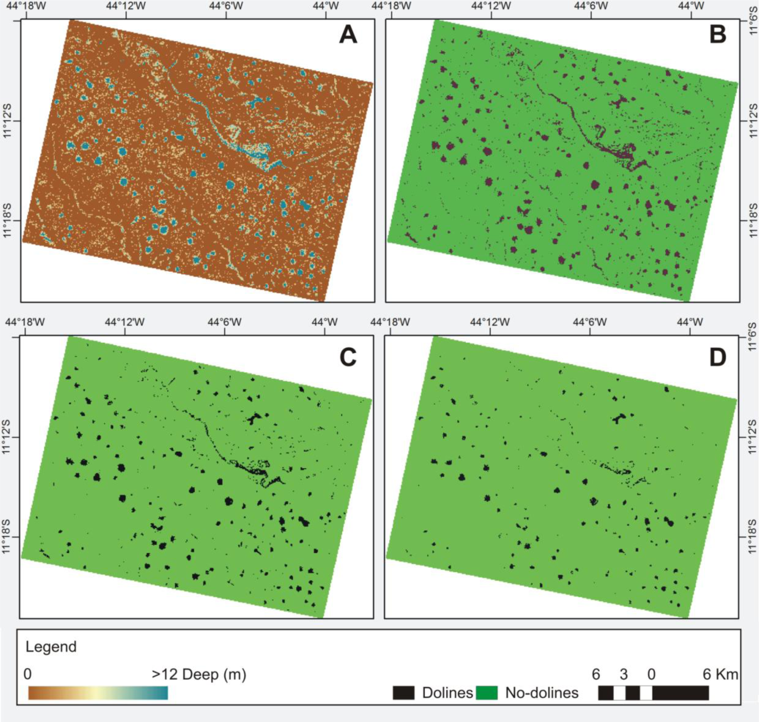
The methodology we used to determine the “sink depth” of closed depressions involved two DEM operations. The first step used the “Fillsink” algorithm from the ArcMap software package [25] that identifies the point or set of adjacent points surrounded by neighbors with higher elevation and rises to the lowest value on the depressions boundary. This procedure then fills all depressions in the DEM, including both those generated from data errors (spurious artifacts) and those that record real topographic features, such as karst depressions (dolines). The second step was to extract the sink depths in these areas by differencing the maps between the sink-filled (“depressionless” DEM) and original DEM (Figure 3).

The difference image (Figure 3C) highlights the different depressions, including the karst enclosed depressions. A binary image is generated from the sink depth image where the depressed areas have value 1, while all other areas have value 0. This binary image is then converted to vector format. The minimum area of depressions corresponds to the spatial resolution of the sensor. However, the polygons show both natural features as well as pits from surface imperfections. Thus, the vectors need to be checked in order to eliminate the errors.

Thus, the key issue is to establish criteria to separate the dolines from the spurious artifacts and other types of depression (e.g., reservoirs or quarries). In this paper, the delimitation of the spurious depressions is derived from threshold values of morphometric attributes, specifically depth, size, and shape.

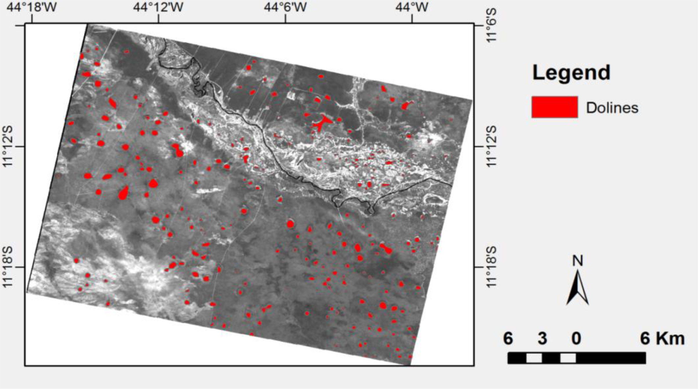
Evaluation of appropriate threshold values to represent the boundary between dolines and the surrounding landscape (“no-dolines”) was obtained by comparing maps of identified dolines with previous mapping of dolines from field validation and interpretation of higher-spatial-resolution imagery (ALOS-PRISM and Google Earth images). The karst features investigated in the study area are easily identified by visual interpretation, as they are characterized by natural moist grassy vegetation where the water table approaches the surface for part of the year, leading to a striking difference in visual appearance from the surrounding vegetation.

We used a range of different empirical threshold values for the minimum sink depth to identify the best threshold value from the maximum accuracy index between manual and automated classification. In assessing classification and change-detection techniques using remotely sensed images, the threshold values for the delimitation of classes are commonly identified from overall accuracy and a Kappa index [57–59]. In this paper we applied the overall accuracy (OA). Performance in identifying true sinkholes is assessed through the intersection of reference and classified polygons. Usually, the polygons obtained by the two methods show distinctions in the dimensions and shapes; but conventional accuracy analysis typically considers only the number of the overlapping polygons. Overall accuracy is calculated by summing the number of polygons classified correctly (True Positive–TP) and dividing by the total number of polygons:

$$\text{OA}=\text{TP}/(\text{TP}+\text{FP}+\text{FN})$$

where the number of polygons misclassified is determined by summing the number of False Negatives (FN) (i.e., no doline identified where one is actually present) and False Positives (FP) (i.e., doline indicated where none exists). This accuracy analysis does not directly assess true negative.

Inevitably, using the proposed method a mapped doline will be represented by more than one polygon. Redundant data (R) must be considered in computing the accuracy index in order to avoid the overestimation. We used the following equation:

$$\text{OA}=(\text{TP}-\text{R})/((\text{TP}+\text{FP}+\text{FN})-\text{R})$$

Therefore comparison between doline classifications with previous maps allows the determination of threshold values for delimiting karst depressions in similar regions and reveals the uncertainties of the method.

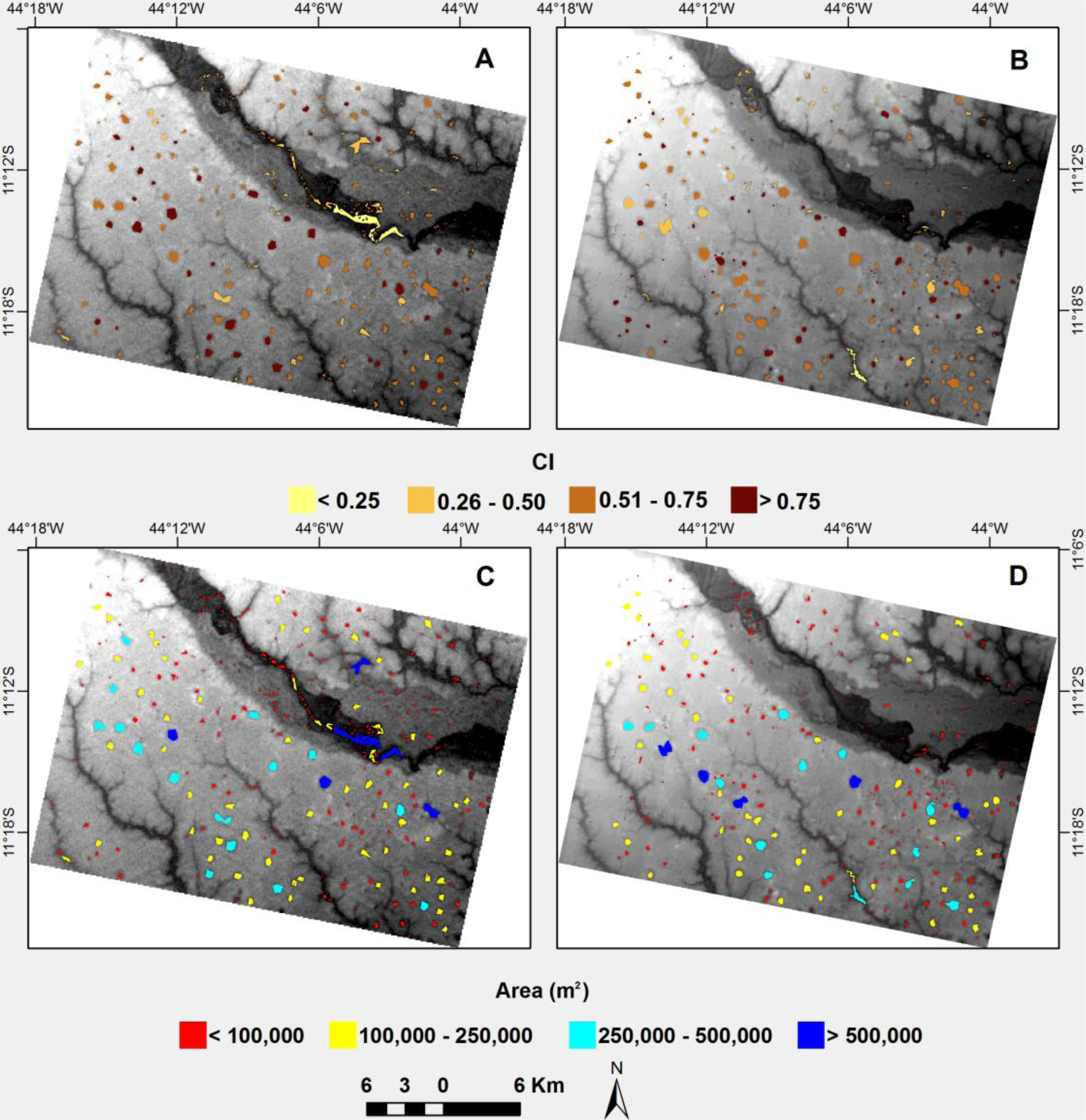
3.3. Morphometric Analysis

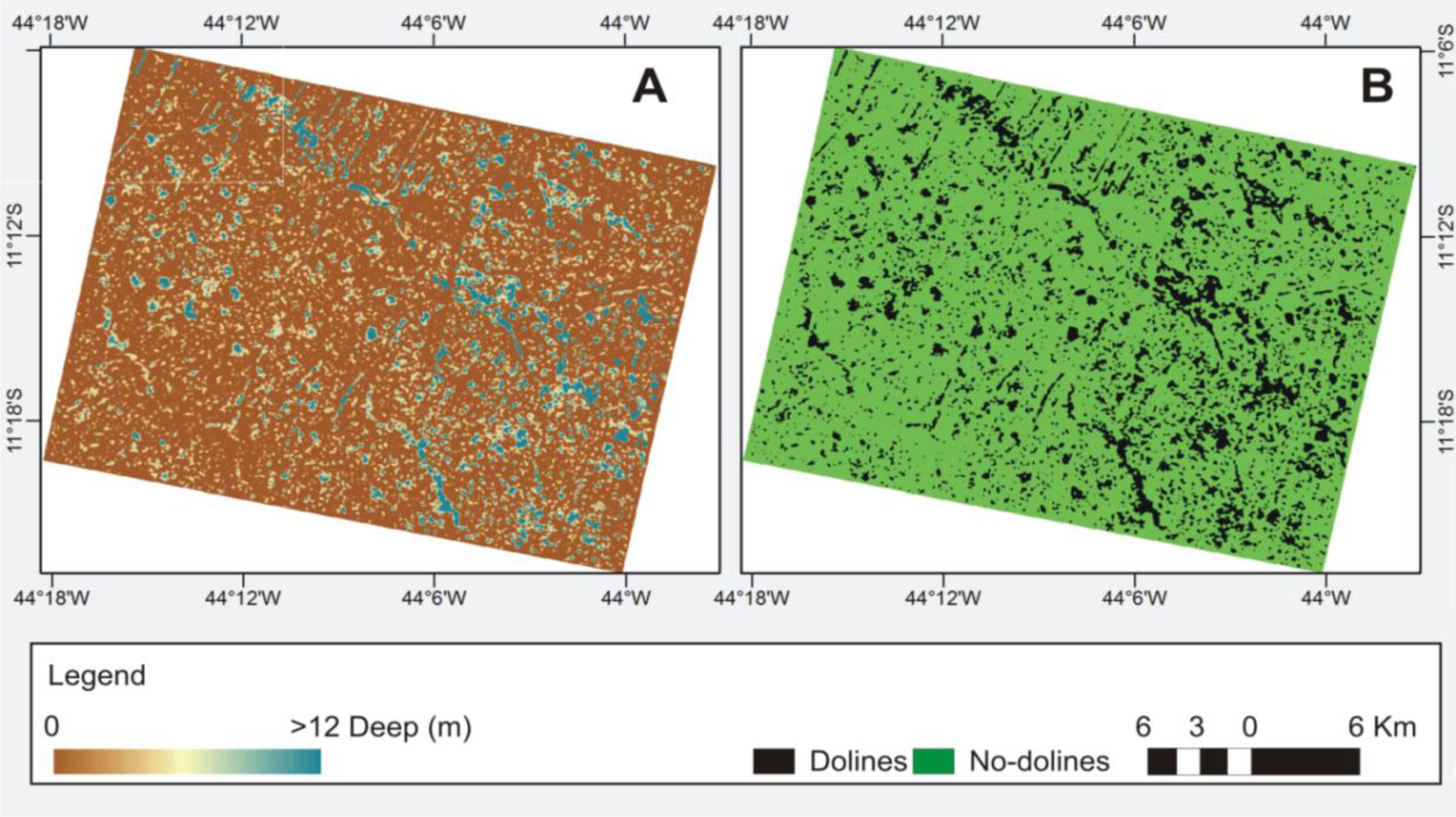
Morphometric analysis may be used to improve the accuracy of predicting doline occurrence and eliminate false dolines. Many of the false dolines can be easily eliminated as being incompatible with known characteristics of karst depressions in the study area (Figure 4). We used the following morphometric attributes to automate delineation of doline polygons: area, perimeter and circularity index (CI). The area and perimeter of the polygons are automatically added to topological vector data structure. We defined a CI based on area and perimeter values using the following equation:

$$\text{CI}=4\pi \text{A}/{\text{P}}^2$$

where A is the area of a polygon and P is its perimeter. A circular shape is represented by value of 1.0, i.e., the maximum value. In contrast, elongated shapes are represented by lower values. The more circular polygons indicate locations of karstic negative relief elements. In addition to the CI values, average and maximum depth were extracted from the DEM for each polygon.

Visual inspection revealed that erroneous polygons generally had a small area, low circularity and were shallow, suggesting that undesirable polygons can be eliminated using threshold value criteria for these morphometric attributes. We superimposed vectors on Google Earth images to identify polygons that represent correctly karst depressions and thereby evaluate the range of morphometric values suitable for use as threshold criteria.

The dolines obtained by morphometric attributes were compared with a reference map using traditional geomorphological procedures such as field surveys and visual interpretation of high-resolution remote sensing image from ALOS/PRISM and Google Earth. In this comparison are evaluated quantities of correct predictions (TP), Type I errors (FP) and Type II errors (FN).

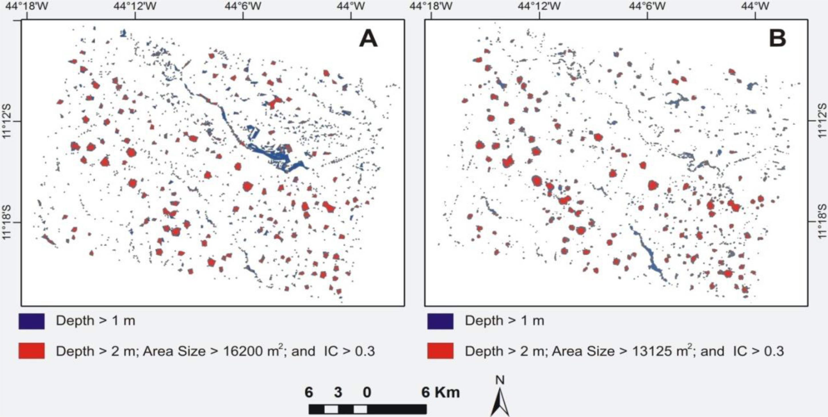
3.4. Enlargement of Doline Polygons

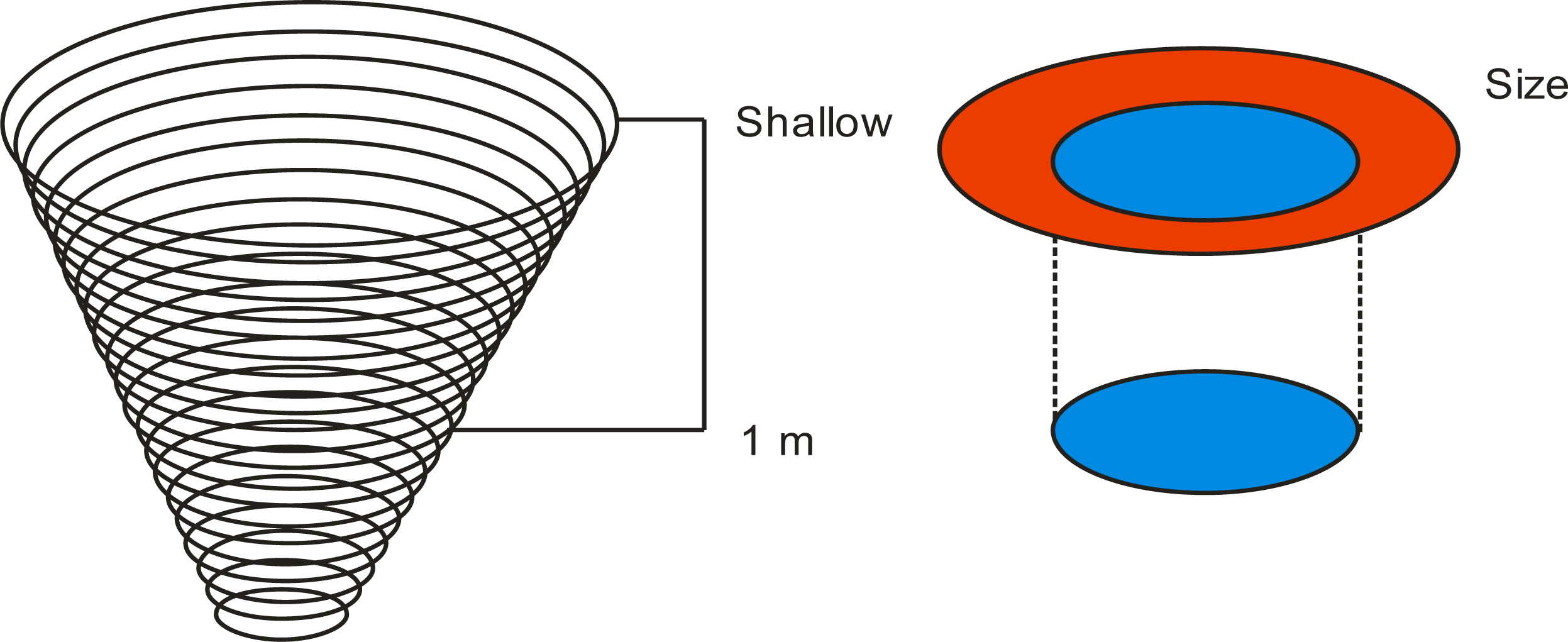
A greater average depth threshold decreases the number of false dolines. However these deeper thresholds do not give the real plan-view area of the dolines. In order to correct for this error, a new mask with a threshold value > 0 m was built and applied to the true dolines previously selected, eliminating the noisy polygons. In doing this, the polygons generated from the depth data are replaced by polygons generated using the shallow depth threshold. This procedure allows having a real area of the doline to be compared with the areas calculated in visual interpretation. However the exact polygon representation is inherently imprecise because the landform itself is hard to define precisely, i.e., the closer you look, the less well-defined the edge becomes. Figure 4 illustrates the hypothetical area of an idealized doline using different thresholds, and how the area decreases with doline depth.

4. Results

4.1. Results of the Visual Interpretation

The reference map was built from the visual interpretation of ALOS/PRISM image (2.5 m); Google Earth images, and detailed field validation. This mapping identified 249 dolines (Figure 5), with the largest sinkholes located on interfluves and smaller sinkholes located closer to the river networks. The comparison between these mapped dolines with those identified through automated classification enables evaluating different threshold values for delimiting karst depressions in similar regions and reveals the uncertainties of the method.

4.2. Results of the Sink-Depth Image

The distribution and depths of closed topographic depressions detected using ASTER-GDEM, SRTM and ALOS data reflected the different spatial resolutions and patterns of noise. For each threshold depth a binary mask image was generated and then represented with polygons. The sink-depth images were classified using threshold values ranging from 1 m. The best threshold for each DEM is defined from the overall accuracy compared to the entire reference map. Therefore a set of classified images made with different thresholds was tested to obtain the optimal value.

Our analysis shows that in our study area, the ASTER-GDEM is susceptible to noise, leading to inaccurate results and visual anomalies and artifacts that represent barriers to its effective utilization for doline detection (Figure 6). Beyond residual cloud anomalies, the ASTER-GDEM has a variety of pervasive artifacts that appear as stripes and other geometric shapes. A significant number of holes in ASTER-GDEM exceed tens of meters and do not correspond to natural dolines (Figure 6). Other studies conducted in karst areas by Guimarães et al. [25] and Siart et al. [26] described difficulties in using the ASTER model in flat areas and in areas with sloping terrain or relief. Previous assessments of ASTER-GDEM accuracy highlight anomalies that prevent its immediate use for a wide range of applications [60,61]. Thus, ASTER-GDEM data are disregarded for further analysis due to their poor performance in karst depression detection.

Figure 7 shows the depth image made from SRTM-DEM threshold values of 1, 2 and 3 m, and a sequence of derived binary masks. Accuracy analyses for different threshold values are presented in

Table 1. Dolines predicted from SRTM-DEM data using different threshold values for sink depth. The comparison is made with 249 true dolines obtained by visual interpretation.

Depth (m)	Numbers of Predicted Dolines	True Positives	Redundant Data	False Positives	False Negatives	Overall Accuracy
1	1,246	256	25	990	18	0.19
2	521	240	35	281	44	0.36
3	297	204	38	93	83	0.49
4	205	152	20	53	117	0.44
5	125	111	9	14	147	0.39

. However, Table 1 presents only the main depth threshold values, in order to demonstrate the convergence to a maximum of overall accuracy; where from it either higher or lower values decrease the accuracy. Using a 1-m threshold depth value resulted in the detection of 1,246 polygons, where the majority is “no dolines” (false positives). In this map 256 true dolines are identified (more than the 249 mapped manually) of which 25 are redundant (i.e., more than one predicted doline demarcates the same natural doline). The increased depth-sink threshold provides a reduction in the number of predicted dolines and false positives and an increased in false negatives. The sink-depth threshold that had the best overall accuracy was the depth of 3 m (0.49), where the errors of omission and commission are approximately equivalent.

Figure 8 shows the depth image from the ALOS/PRISM-DEM and binary masks made with the same three threshold values.

Table 2. Dolines predicted using different threshold values for sink depth from ALOS/PRISM-DEM data. The comparison is made with true dolines (249) obtained by visual interpretation.

Depth (m)	Numbers of Predicted Dolines	True Positives	Redundant Data	False Positives	False Negatives	Overall Accuracy
1	1,276	271	45	1,005	23	0.18
2	590	254	59	336	54	0.33
3	348	205	38	143	82	0.43
4	230	160	38	70	127	0.38
5	176	133	36	43	152	0.33

shows the threshold values for each sink-depth using ALOS/PRISM-DEM and its corresponding overall accuracy. The best-fit results are obtained for deeper than 3 m, where the overall accuracy is 0.43. Thus threshold value for the ALOS/PRISM-DEM is similar to that for the SRTM-DEM and both perform well in identifying medium-size landforms. ALOS/PRISM-DEMs have limitations in the presence of clouds, and SRTM-DEMs have problems with fine-scale distortions. In this paper, the image used had a small cloudy area that was disregarded. The radar-based SRTM-DEM does not have this problem.

4.3. Results of the Morphometric Analysis

Additionally, in order to increase the overall accuracy we developed a morphometric analysis that considers area and CI attributes. At this stage we analyzed the polygons of sinkholes with depths greater than 3 m (depth with highest accuracy among those tested with the SRTM-DEM) and 2 m (for reconciling high value of overall accuracy and high number of true positives). Figure 9 shows the morphometric attributes for the depression polygons deeper than 2 m (since it includes all polygons with depth values more than 3 m).

Initially, the threshold analysis was done for the area and then for CI. In this text, tables of morphometric attributes show only the main results, highlighting the convergence to an optimal threshold value with maximum overall accuracy. For area-size analysis from SRTM-DEM, the best overall accuracy (0.52) was obtained from the following conditions: depth > 2 m and area > 16,200 m² (

Table 3. Dolines predicted using the area attribute derived from the doline depth > 2 m (SRTM-DEM). Comparison is made with the actual dolines (249) mapped by visual interpretation.

Area (m2)	Numbers of Predicted Dolines	True Positives	Redundant Data	False Positives	False Negatives	Overall Accuracy
>8,100	293	189	7	104	67	0.52
>16,200	229	164	1	65	86	0.52
>24,300	179	143	0	36	106	0.50
>32,400	158	132	0	26	117	0.48

). This combination resulted in values of overall accuracy greater than obtained for depth > 3 m (0.49) (Table 1) or supplemented by the restriction of area > 8,100 m² (0.49) (

Table 4. Dolines predicted using the area attribute calculated from the doline depth > 3 m (SRTM-DEM). The comparison is made with actual dolines (249) mapped by visual interpretation.

Area (m2)	Numbers of Predicted Dolines	True Positives	Redundant Data	False Positives	False Negatives	Overall Accuracy
>8,100	190	150	7	40	106	0.49
>16,200	157	131	1	26	119	0.47
>24,300	123	110	1	13	140	0.42
>32,400	108	96	0	12	153	0.37

). The area attribute eliminated mainly small spurious artifacts (False Positives and False Negatives).

The threshold analysis for the CI allowed a little improvement in the already obtained overall accuracy. Assuming a CI > 3 resulted in an overall accuracy of 0.53 (

Table 5. Predicted dolines using SRTM-DEM and circularity index attribute for dolines depth > 2 m and area > 16,200. The comparison is made with true dolines (249) obtained by visual interpretation.

CI	Numbers of Predicted Dolines	True Positives	Redundant Data	False Positives	False Negatives	Overall Accuracy
>0.3	224	164	1	60	86	0.53
>0.35	221	162	1	59	88	0.52
>0.4	216	160	1	56	90	0.52

). This procedure eliminated large and long polygons corresponding mainly to fluvial features. Thus, the best overall accuracy for the doline delimitation using SRTM-DEM has the following constraints: depth > 2 m; area > 16,200 m² and CI > 0.3.

ALOS/PRISM-DEM demonstrated that the best overall accuracy was obtained by the following combination: area > 16,200 m² and depth > 2 m (0.53) (

Table 6. Predicted dolines using area attribute from dolines depth > 2 m (ALOS/PRISM-DEM). The comparison is made with true dolines (249) obtained by visual interpretation.

Area (m2)	Numbers of Predicted Dolines	True Positives	Redundant Data	False Positives	False Negatives	Overall Accuracy
>8,125	263	176	8	87	81	0.50
>10,625	237	170	6	67	85	0.52
>13,125	211	162	4	49	91	0.53
>15,625	195	153	0	42	96	0.53
>18,125	182	146	0	36	103	0.51

and

Table 7. Predicted dolines using area attribute from dolines depth > 3 m (ALOS/PRISM-DEM). The comparison is made with true dolines (249) obtained by visual interpretation.

Area (m2)	Numbers of Predicted Dolines	True Positives	Redundant Data	False Positives	False Negatives	Overall Accuracy
>625	316	190	26	126	85	0.44
>3,125	225	155	8	70	102	0.46
>5,625	179	138	3	41	114	0.47
>8,125	157	125	0	32	124	0.44
>10,625	144	116	0	28	133	0.42

). This overall accuracy was better than simply restricting depth to > 2 m (0.33) or depth to > 3 m (0.43) (Table 2). The best overall accuracy from the ALOS/PRISM-DEM was slightly higher than that for the SRTM-DEM.

As for the SRTM-DEM, the threshold analysis of CI in the ALOS/PRISM-DEM allowed a slight improvement in the overall accuracy (0.53) (

Table 8. Predicted dolines using ALOS/PRISM-DEM and circularity index attribute for dolines depth > 2 m and area > 13,125 m². The comparison is made with true dolines (249) obtained by visual interpretation.

CI	Numbers of Predicted Dolines	True Positives	Redundant Data	False Positives	False Negatives	Overall Accuracy
>0.3	207	161	4	46	92	0.53
>0.35	201	157	4	44	96	0.52
>0.4	197	153	3	44	99	0.51

). At this morphometric attribute, both the DEMs showed the same threshold value (0.3). Thus, the best configuration for ALOS/PRISM-DEM considers the following constrains: depth > 2 m; area > 13,125 m² and IC > 0.3.

Once appropriate threshold values are defined from a reference area, they can be applied to other similar locations. Morphometric analysis identified little more than half of the actual dolines, which may reduce the need for visual interpretation. Figure 10 shows all polygons > 1 m initially obtained with sink-depth images and the polygons obtained after the restrictions by morphometric attributes for DEMs from SRTM and ALOS/PRISM.

The differences in spatial resolution of the DEMs generate singular shapes for the depressions. Due to the high resolution of the ALOS/PRISM image, the depressions are better defined in them, whereas in the SRTM-DEM the depression outlines are less detailed. Despite shape differences the SRTM–DEM indicates the great majority of the points described by ALOS/PRISM-DEM.

4.5. Results of the Adjustment of the Size of Dolines

Larger doline polygons with better overall accuracy from SRTM and ALOS data are associated with a threshold depth of 2 m. This procedure increased the areas of sinkholes, making them more consistent with visual interpretation. Figure 11 shows in detail the effect caused for some sinkholes.

4.6. Spatial Distribution of Dolines

An analysis of the spatial distribution of morphometric attributes shows a correlation with structures and geological settings. The deepest depressions are connected to the main drainage network. In particular, the largest dolines show a NE-SE trend in the interfluve region following the preferred direction of regional geological structures and the drainage network.

With regard to morphological manifestations, two landscape types are distinguished in the study region: the upland karst and the incised river valleys. The plateau karst shows inter-relationships between surface and sub-surface drainage, developing karstic processes. The upland surfaces exhibit a parallel drainage pattern, with dolines concentration along the interfluves. The dolines are all on the undissected upper (older) landscape surface, indicating that dolines increase in number through time, as observed in other tropical areas [62]. The lower elevation dissected surface is a region of well-developed fluvial features, where few dolines occur on river terraces and low-elevation, erosion surfaces.

5. Conclusions

Semi-automated landform classification using DEMs provides several advantages: fast acquisition of data over large areas at low cost, analysis of inaccessible zones, reduction of human errors by eliminating manual classification steps, ready comparison of results derived from different datasets, and the reduction in processing time. Our methodology for mapping karst depressions combines morphometric analysis with a minimum threshold value for the sink depth to identify karst depressions. However, some depressions selected by sink depth are actually data errors introduced in generating the surface and should be interpreted with prudence. We suggest a method for the separation of real from incorrectly identified topographic features. The identification of the optimal threshold values for assessing morphometric attributes was made from the highest overall accuracy, considering a reference map built from visual interpretation. These threshold values are limited to areas with similar environmental conditions. Thus studies in new locations must first define the best thresholds using a test area.

In this work, the ASTER-GDEM had severe limitations in the detection of karst features. However, this is not a general criticism of the ASTER-GDEM, which may perform better in other areas or other problems. The GDEM data generation process consists of scene selection, scene division, same-path mosaic generation, stacking, sticking, and filtering for both elevation data and water-body data [63]. Despite this processing some images may contain imperfections, which are being fixed in another version of the ASTER-GDEM product. Therefore, the doline detection considering other areas or new products may get better results.

SRTM-DEM and ALOS/PRISM-DEM identify more than half of the true dolines with an overall accuracy of approximately 0.5. The ALOS/PRISM-DEM has potentially serious limitations in the presence of clouds, whereas the SRTM-DEM is insensitive to cloud cover. However, the coarser resolution of the SRTM-DEM limits its utility in delineating fine-scale karst features. Practically all the larger sinkholes detected by ALOS were also identified by the SRTM. Therefore SRTM and ALOS data are reasonably well suited for use in large-scale mapping of karst features in Central Brazil.

The algorithm results could be improved by considering three distinct aspects: (a) the addition of other DEM attributes or polygon geometry; (b) the use of DEM with higher spatial resolution (e.g., airborne laser scanning); and (c) the application of other complementary data to the DEM, such as multi-spectral images.

In detecting sinkholes other morphometric information can be used, providing an additional component for spatial analysis. Siart et al. [26] used the following DEM attributes to assist doline detection: slope, aspect and curvature. However the results were difficult to interpret, due to the visual complexity of the image, and did not contribute significantly to doline detection. With respect to the polygon geometry the eccentricity of an ellipse remains to be tested [64], although for the present study area this should help little, because the dolines are circular. Thus, tests with other morphometric attributes may provide a little improvement in accuracy of the algorithm in the general application. The main improvements probably lie in the other two mentioned alternatives.

The use of images with higher spatial resolution undoubtedly enables better detection of sinkholes. A particularly promising area for future study is the acquisition of the morphometric attributes from LiDAR (Light Detecting and Ranging) data, which has impressive accuracy for detecting sinkholes and estimating subsidence rates [65–68]. Another major advantage of utilizing laser scanning technology is its canopy penetration ability. However, many areas do not have this type of data.

Although beyond the scope of this paper, the use of classification of multi-spectral images can significantly increase the detection accuracy of dolines. Remote-sensing data, whether airborne or satellite-based, offer an alternative way for the doline detection considering karst-dependent features (e.g., sedimentary infills and vegetation). Thus the depressions can locally modify environmental variables: soil moisture, water stagnation, soil erosion and sedimentation, and spatial distributions of the vegetation with relative presence of dominant species. In this approach, some works [25,26] demonstrates that the combination of DEMs and high-resolution satellite imagery produce the best results in karst geomorphological research.

References

1. Galve, J.P.; Gutiérrez, F.; Lucha, P.; Guerrero, J.; Bonachea, J.; Remondo, J.; Cendrero, A. Probabilistic sinkhole modelling for hazard assessment. Earth Surf. Proc. Landf 2009, 34, 437–452. [Google Scholar]
2. Gutiérrez, F.; Galve, J.P.; Guerrero, J.; Lucha, P.; Cendrero, A.; Remondo, J.; Bonachea, J.; Gutiérrez, M.; Sánchez, J.A. The origin, typology, spatial distribution, and detrimental effects of the sinkholes developed in the alluvial evaporite karst of the Ebro River valley downstream Zaragoza city (NE Spain). Earth Surf. Proc. Landf 2007, 32, 912–928. [Google Scholar]
3. Soriano, M.A.; Simón, J.L. Alluvial dolines in the central Ebro Basin, Spain: A spatial and developmental hazard analysis. Geomorphology 1995, 11, 295–309. [Google Scholar]
4. White, E.L.; Gert, A.; White, W.B. The influence of urbanization in sinkhole development in central Pennsylvania. Environ. Geol. Water Sci 1986, 8, 91–97. [Google Scholar]
5. Soriano, M.A. Characteristics of the alluvial dolines developed because of gypsum dissolution in the central Ebro Basin. Z. Geomorphol. Suppl 1992, 85, 59–72. [Google Scholar]
6. Castañeda, C.; Gutiérrez, F.; Manunta, M.; Galve, J.P. DInSAR measurements of ground deformation by sinkholes, mining subsidence, and landslides, Ebro River, Spain. Earth Surf. Proc. Landf 2009, 34, 1562–1574. [Google Scholar]
7. Ford, D.C.; Williams, P.W. Karst Geomorphology and Hydrology; Unwin Hyman: London, UK, 1989. [Google Scholar]
8. Trudgill, S. Limestone Geomorphology; Longman Group: New York, NY, USA, 1985. [Google Scholar]
9. Kresic, N. Remote sensing of tectonic fabric controlling groundwater flow in Dinaric Karst. Remote Sens. Environ 1995, 53, 85–90. [Google Scholar]
10. Florea, L. Using state-wide GIS data to identify the coincidence between sinkholes and geologic structure. J. Cav. Karst. Stud 2005, 67, 120–124. [Google Scholar]
11. Closson, D.; Karaki, N.A. Salt karst and tectonics: Sinkholes development along tension cracks between parallel strike-slip faults, Dead Sea, Jordan. Earth Surf. Proc. Landf 2009, 34, 1408–1421. [Google Scholar]
12. Doerfliger, N.; Jeannin, P.Y.; Zwahlen, F. Water vulnerability assessment in karst environments: A new method of defining protection areas using a multi-attribute approach and GIS tools (EPIK method). Environ. Geol 1999, 39, 165–176. [Google Scholar]
13. Van Stempvoort, D.; Evert, L.; Wassenaar, L. Aquifer vulnerability index: A GIS compatible method for groundwater vulnerability mapping. Can. Water Resour. J 1993, 18, 25–37. [Google Scholar]
14. Quinn, P.; Beven, K.; Chevallier, P.; Planchon, O. The prediction of hillslope flow paths for distributed hydrological modelling using digital terrain models. Hydrol. Proc 1991, 5, 59–79. [Google Scholar]
15. Zhang, W.; Montgomery, D.R. Digital elevation model grid size, landscape representation and hydrologic simulations. Water Resour. Res 1994, 30, 1019–1028. [Google Scholar]
16. Tucker, G.E.; Hancock, G.R. Modelling landscape evolution. Earth Surf. Proc. Landf 2010, 35, 28–50. [Google Scholar]
17. Carvalho Júnior, O.A.; Guimarães, R.F.; Freitas, L.; Gomes-Loebmann, D.; Gomes, R.A.; Martins, E.S.; Montgomery, D.R. Urbanization impacts upon catchment hydrology and gully development using mutli-temporal digital elevation data analysis. Earth Surf. Proc. Landf 2010, 35, 611–617. [Google Scholar]
18. Bolongaro-Crevenna, A.; Torres-Rodriguez, V.; Sorani, V.; Frame, D.; Arturo Ortiz, M. Geomorphometric analysis for characterizing landforms in Morelos State, Mexico. Geomorphology 2005, 67, 407–422. [Google Scholar]
19. Podobnikar, T. Detecting mountain peaks and delineating their shapes using digital elevation models, remote sensing and geographic information systems using autometric methodological procedures. Remote Sens 2012, 4, 784–809. [Google Scholar]
20. Wood, J.D. The Geomorphologic Characterization of Digital Elevation Models. University of Leicester, London, UK, 1996. [Google Scholar]
21. Segura, F.S.; Pardo-Pascual, J.E.; Rosselló, V.M.; Fornós, J.J.; Gelabert, B. Morphometric indices as indicators of tectonic, fluvial and karst processes in calcareous drainage basins, South Menorca Island, Spain. Earth Surf. Proc. Landf 2007, 32, 1928–1946. [Google Scholar]
22. Lyew-Ayee, P.; Viles, H.A.; Tucker, G.E. The use of GIS-based digital morphometric techniques in the study of cockpit karst. Earth Surf. Proc. Landf 2007, 32, 165–179. [Google Scholar]
23. Piccini, L.; Landelli, N. Tectonic uplift, sea level changes and Plio-Pleistocene evolution of a coastal karst system: the Mount Saint Paul (Palawan, Philippines). Earth Surf. Proc. Landf 2010, 36, 594–609. [Google Scholar]
24. Antonic, O.; Hatic, D.; Pernar, R. DEM-based depth in sink as an environmental estimator. Ecol. Model 2001, 138, 247–254. [Google Scholar]
25. Guimarães, R.F.; Carvalho Junior, O.A.; Souza Martins, E.M.; Carvalho, A.P.F.; Gomes, R.A.T. Detection of karst depression by ASTER image in the Bambui Group, Brazil. Proc. SPIE 2005, 5983, 328–339. [Google Scholar]
26. Siart, C.; Bubenzer, O.; Eitel, B. Combining digital elevation data (SRTM/ASTER), high resolution satellite imagery (Quickbird) and GIS for geomorphological mapping: A multi-component case study on Mediterranean karst in Central Crete. Geomorphology 2009, 112, 106–121. [Google Scholar]
27. Pardo-Igúzquiza, E.; Valsero, J.J.D.; Dowd, P.A. Automatic detection and delineation of karst terrain depressions and its application in geomorphological mapping and morphometric analysis. Acta. Carsologica 2013, 42, 17–24. [Google Scholar]
28. Marks, D.; Dozier, J.; Frew, J. Automated basin delineation from digital elevation data. Geo-Processing 1984, 2, 299–311. [Google Scholar]
29. Jenson, S.K.; Domingue, J.O. Extracting topographic structure from digital elevation data for geographical information system analysis. Photogramm. Eng. Remote Sens 1987, 54, 1593–1600. [Google Scholar]
30. Tianqi, A.; Takeuchi, K.; Ishidaira, H.; Yoshitani, J.; Fukami, K. Development and application of a new algorithm for automated pit removal for grid DEMs. Hydrol. Sci. J 2003, 48, 985–997. [Google Scholar]
31. Soille, P.; Vogt, J.; Colombo, R. Carving and adaptive drainage enforcement of grid digital elevation models. Water Resour. Res 2003, 39, 1366–1375. [Google Scholar]
32. Grimaldi, S.; Nardi, F.; Benedetto, F.; Istanbulluoglu, E.; Brás, R.L. A physically-based method for removing pits in digital elevation models. Adv. Water Resour 2007, 30, 2151–2158. [Google Scholar]
33. Obu, J.; Podobnikar, T. Algorithm for karst depression recognition using digital terrain models. Geodetski Vestnik 2013, 57, 260–270. [Google Scholar]
34. Kass, M; Witkin, A; Terzopoulous, D. Snakes: Active contour models. Int. J. Comput. Vis 1988, 1, 321–331. [Google Scholar]
35. Rahimi, M.; Alexander, E.C., Jr. Locating Sinkholes in LIDAR Coverage of a Glacio-Fluvial Karst, Winona County, MN. Proceedings of the 13th Multidisciplinary Conference on Sinkholes and the Engineering and Environmental Impacts of Karst, Carlsbad, CA, USA, 1 May–15 August 2013; pp. 469–480.
36. Karmann, I. Evolução Dinâmica Atual do Sistema Cárstico do Alto Vale do Ribeira de Iguape, Sudeste do Estado de São Paulo; São Paulo. Universidade de São Paulo, São Paulo, Brazil, 1994. [Google Scholar]
37. Karmann, I.; Sánchez, L.E. Distribuição das rochas carbonáticas e províncias espeleológicas do Brasil. Espeleo-Tema 1979, 13, 105–167. [Google Scholar]
38. Carvalho Júnior, O.A.; Berbet-Born, M.; Martins, E.S.; Guimarães, R.F.; Gomes, R.A.T. Ambientes Cársticos. In Geomorfologia: Conceitos e Tecnologias Atuais; Florenzano, T.G., Ed.; Oficina de Textos: São Paulo, Brazil, 2008; Volume 1, pp. 183–218. [Google Scholar]
39. Castro, P.T.A. Os Conglomerados da Borda SW do Cráton do São Francisco Junto a Porção S da Faixa Brasília: Sedimentologia e Relações Estratigráficas com as Rochas do Grupo Bambuí. Universidade de Brasília, Brasília, Brazil, 1997. [Google Scholar]
40. Castro, P.T.A.; Dardenne, M.A. The sedimentology stratigraphy and tectonic context of the São Francisco Supergroup at the southern boundary of the São Francisco craton, Brazil. Rev. Brasil. Geociência 2000, 30, 345–437. [Google Scholar]
41. Martins-Neto, M.A.; Pedrosa-Soares, A.C.; Lima, S.A.A. Tectono-sedimentary evolution of sedimentary basins from Late Paleoproterozoic to Late Neoproterozoic in the São Francisco Craton and Araçuaí Fold belt, Eastern Brazil. Sediment. Geol 2001, 141/142, 343–370. [Google Scholar]
42. Abrams, M. The Advanced Spaceborne Thermal Emission and Reflection Radiometer (ASTER): Data products for the high spatial resolution imager on NASA’s Terra platform. Int. J. Remote Sens 2000, 21, 847–859. [Google Scholar]
43. Farr, T.G.; Rosen, P.A.; Caro, E.; Crippen, R.; Duren, R.; Hensley, S.; Kobrick, M.; Paller, M.; Rodriguez, E.; Roth, L.; et al. The Shuttle Radar Topography Mission. Rev. Geophys 2007. [Google Scholar] [CrossRef]
44. Smith, B.; Sandwell, D. Accuracy and resolution of Shuttle Radar Topography Mission data. Geophys. Res. Lett 2003, 30, 1467. [Google Scholar]
45. Van Zyl, J.J. The Shuttle Radar Topography Mission (SRTM): A breakthrough in remote sensing of topography. Acta. Astronaut 2001. [Google Scholar] [CrossRef]
46. Rabus, B.; Eineder, M.; Roth, A.; Bamler, R. The shuttle radar topography mission—A new class of digital elevation models acquired by spaceborne radar. Photogramm. Eng. Remote Sens 2003, 57, 241–262. [Google Scholar]
47. Rossetti, D.F. Multiple remote sensing techniques as a tool for reconstructing late Quaternary drainage in the Amazon lowland. Earth Surf. Proc. Landf 2010, 35, 1234–1239. [Google Scholar]
48. Petersen, G.; Sutcliffe, J.V.; Fohrer, N. Morphological analysis of the Sudd region using land survey and remote sensing data. Earth Surf. Proc. Landf. 2008, 33, 1709–1720. [Google Scholar]
49. Maruya, M.; Ohyama, H. Accurate DEM and Ortho-Rectified Image Production from ALOS/PRISM. Proceedings of the 2008 IEEE International Geoscience and Remote Sensing Symposium, Boston, WA, USA, 7–11 July 2008; pp. 185–188.
50. Tadono, T.; Shimada, M.; Watanabe, M.; Rosenqvist, A. Overview of ALOS research and science program. Proc. SPIE 2004. [Google Scholar] [CrossRef]
51. Gruen, A.; Kocaman, S.; Wolff, K. Calibration and validation of EARLY ALOS/PRISM images. J. Jpn. Soc. Photogramm. Remote Sens 2007, 46, 24–38. [Google Scholar]
52. Kocaman, S.; Gruen, A. Orientation and Calibration of ALOS/PRISM Imagery. Proceedings of the 2007 ISPRS Hannover Workshop: High-Resolution Earth Imaging for Geospatial Information, Hanover, Germany, 29 May–21 June 2007; p. 6.
53. Saunier, S.; Santer, R.; Goryl, P.; Gruen, A.; Wolf, K.; Bouvet, M.; Viallefont, F.; Chander, G.; Rodriguez, Y.; Mambimba, A. The Contribution of the European Space Agency to the ALOS PRISM/AVNIR-2 Commissioning Phase. Proceedings of the IEEE International Geoscience and Remote Sensing Symposium, Barcelona, Spain, 1 July 2007; pp. 208–211.
54. Brazilian government. Avaliação Planialtimétrica de Dados ALOS/PRISM Estudo de Caso: Itaguaí—RJ; Instituto Brasileiro de Geografia e Estatística: Rio de Janeiro, Brazil, 2009. [Google Scholar]
55. Futamura, N.; Takaku, J.; Suzuki, H.; Iijima, T.; Tadono, T.; Matsuoka, M.; Shimada, M.; Igarashi, T.; Shibasaki, R. High Resolution DEM Generation from ALOS PRISM Data-Algorithm Development and Evaluation. Proceedings of the IGARSS 2002 IEEE International Geoscience and Remote Sensing Symposium, Toronto, Canada, 24–28 June 2002; 1, pp. 405–407.
56. Geomatics, P.C.I. PCI Geomatica OrthoEngine User Guide, version 10.3; GEOMATIC: Richmond Hill, ON, Canada, 2010. [Google Scholar]
57. Carvalho Júnior, O.A.; Guimarães, R.F.; Gillespie, A.R.; Silva, N.C.; Gomes, R.A.T. A new approach to change vector analysis using distance and similarity measures. Remote Sens 2011, 3, 2473–2493. [Google Scholar]
58. Congalton, R.; Green, K. Assessing the Accuracy of Remotely Sensed Data: Principles and Practices; CRC and Lewis Press: Boca Raton, FL, USA, 1999. [Google Scholar]
59. Fung, T.; Le Drew, E. Application of principal components analysis to change detection. Photogramm. Eng. Remote Sens 1987, 53, 1649–1658. [Google Scholar]
60. Hirt, C.; Filmer, M.S.; Featherstone, W.E. Comparison and validation of recent freely-available ASTER-GDEM ver1, SRTM ver4.1 and GEODATA DEM-9S ver3 digital elevation models over Australia. Aust. J. Earth Sci 2010, 57, 337–347. [Google Scholar]
61. Reuter, H.I.; Nelson, A.; Strobl, P.; Mehl, W.; Jarvis, A. A First Assessment of ASTER GDEM Tiles for Absolute Accuracy, Relative Accuracy and Terrain Parameters. Proceedings of the IGARSS 2009 Geoscience and Remote Sensing Symposium, Cape Town, South Africa, 12–17 July 2009; 5, pp. 240–243.
62. Day, M. Doline morphology and development in Barbados. Ann. Assoc. Am. Geogr 1983, 73, 206–219. [Google Scholar]
63. Fujisada, H.; Urai, M.; Iwasaki, A. Technical methodology for ASTER global DEM. IEEE Trans. Geosci. Remote Sens 2012, 50, 3725–3736. [Google Scholar]
64. Doctor, D.H.; Young, J.A. An Evaluation of Automated GIS Tools for Delineating Karst Sinkholes and Closed Depressions from 1-Meter LIDAR-Derived Digital Elevation Data. Proceedings of the 13th Multidisciplinary Conference on Sinkholes and the Engineering and Environmental Impacts of Karst, Carlsbad, NM, USA, 1 May–15 August 2013; pp. 449–458.
65. Filin, S.; Baruch, A. Detection of sinkhole hazards using airborne laser scanning data. Photogramm. Eng. Remote Sens 2010, 76, 577–587. [Google Scholar]
66. Filin, S.; Baruch, A.; Avni, Y.; Marco, S. Sinkhole characterization in the Dead Sea area using airborne laser scanning. Nat. Hazard 2011, 58, 1135–1154. [Google Scholar]
67. Shaw-Faulkner, M.G.; Stafford, K.W.; Bryant, A.W. Delineation and Classification of Karst Depressions using LiDAR: Fort Hood Military Installation, Texas. Proceedings of the 13th Multidisciplinary Conference on Sinkholes and the Engineering and Environmental Impacts of Karst, Carlsbad, NM, USA, 1 May–15 August 2013; pp. 459–468.
68. Waltham, T.; Bell, F; Culshaw, M. Ground investigation in sinkhole terrains. In Sinkholes and Subsidence; Springer: Chichester, UK, 2005; pp. 181–204. [Google Scholar]
Figure 1. Study area location.
Remotesensing 06 00330f1
Figure 2. Karst depression covered by herbaceous vegetation and stagnant surface water.
Remotesensing 06 00330f2
Figure 3. Methodological procedures to determine the terrain attribute of sink depth. Digital elevation model (A) (DEM) Fillsink minus (B) original DEM results in the (C) sink-depth distribution.
Remotesensing 06 00330f3
Figure 4. Hypothetical dolines enlargement from threshold depths equal to 1 m and “shallow” (i.e., > 0 m).
Remotesensing 06 00330f4
Figure 5. Reference map from the visual interpretation of ALOS/PRISM and Google Earth images.
Remotesensing 06 00330f5
Figure 6. (A) Depth image and (B) its derived binary mask made from ASTER-GDEM data using threshold value of 1 m.
Remotesensing 06 00330f6
Figure 7. Depth image from (A) SRTM-DEM and binary mask images made with sink-depth thresholds of (B) 1 m, (C) 2 m and (D) 3 m.
Remotesensing 06 00330f7
Figure 8. Depth image from (A) ALOS/PRISM-DEM and binary mask images made considering sink-depth thresholds of (B) 1 m, (C) 2 m and (C) 3 m.
Remotesensing 06 00330f8
Figure 9. Spatial distribution of dolines considering the following attributes: area from (A) SRTM-DEM and (B) ALOS/PRISM-DEM, and circularity indexes from (C) SRTM-DEM and (D) ALOS/PRISM-DEM.
Remotesensing 06 00330f9
Figure 10. Comparison between delimited dolines from depth > 1 (blue polygon) and using the morphometric analysis (red polygon) that provides a significant decrease of sinkholes. (A) SRTM-DEM and (B) ALOS/PRISM-DEM.
Remotesensing 06 00330f10
Figure 11. The sinkholes obtained from the morphometric attributes have increased their sizes considering a shallow depth from the (A) SRTM-DEM and (B) ALOS/PRISM-DEM.
Remotesensing 06 00330f11