Estimates of Forest Growing Stock Volume for Sweden, Central Siberia, and Québec Using Envisat Advanced Synthetic Aperture Radar Backscatter Data

 ,
,  ,
,
Abstract
: A study was undertaken to assess Envisat Advanced Synthetic Aperture Radar (ASAR) ScanSAR data for quantifying forest growing stock volume (GSV) across three boreal regions with varying forest types, composition, and structure (Sweden, Central Siberia, and Québec). Estimates of GSV were obtained using hyper-temporal observations of the radar backscatter acquired by Envisat ASAR with the BIOMASAR algorithm. In total, 5.3·106 km2 were mapped with a 0.01° pixel size to obtain estimates representative for the year of 2005. Comparing the SAR-based estimates to spatially explicit datasets of GSV, generated from forest field inventory and/or Earth Observation data, revealed similar spatial distributions of GSV. Nonetheless, the weak sensitivity of C-band backscatter to forest structural parameters introduced significant uncertainty to the estimated GSV at full resolution. Further discrepancies were observed in the case of different scales of the ASAR and the reference GSV and in areas of fragmented landscapes. Aggregation to 0.1° and 0.5° was then undertaken to generate coarse scale estimates of GSV. The agreement between ASAR and the reference GSV datasets improved; the relative difference at 0.5° was consistently within a magnitude of 20–30%. The results indicate an improvement of the characterization of forest GSV in the boreal zone with respect to currently available information.1. Introduction
The amount and spatial distribution of forest resources in the boreal zone are highly debated as they are often roughly quantified and seldom verified [1,2]. Continuous changes to forest resource distribution, due to changes in land use, natural and anthropogenic disturbances and recovery, and physiological or metabolic changes result in a need for periodic updating [3]. Gaps and errors in available datasets imply that investigations based on such records (e.g., for assessing carbon stocks) can suffer from substantial uncertainties.
For the boreal zone, traditional field survey techniques have substantial limitations to achieve accurate and repeated characterization of forest conditions [4–6]. In addition, financial and logistical constraints may lead to inconsistent quality of field measurements of forest resources. The Nordic European countries can afford accurate forest inventories undertaken on a regular basis with short cycles, such as five year cycles [7]. Advanced field survey techniques are implemented to increase coverage and timeliness of the collected data. In contrast, the completion of a country-wide inventory of Russia spans at least a decade and the precision of the field survey depends to a large degree on land accessibility and financial means to support such surveys. In Siberia and the Far East, more than 50% of the forests have not been revisited for more than 20 years after the last inventory due to budget restrictions [8]. In Québec, the temperate and southern boreal forest areas (roughly 40% of the provincial forest land) are systematically and intensively inventoried each decade [9].
Satellite remote sensing supports mapping and monitoring of forest resources on a large scale because of its synoptic view, frequent revisit capability, relative low cost, and sensitivity of the observable to either biophysical or structural properties of forests. Satellite optical images in conjunction with plot-wise measurements from forest field inventory have been used to generate country-wide [10–12], continental [13,14], and global [15] data products of above-ground biomass, growing stock volume and canopy cover fraction. LiDAR (Light Detection And Ranging) point-wise measurements have been implemented in combination with either in situ or two-dimensional data from optical imagery to provide spatially explicit estimates of forest canopy height [16,17], above-ground biomass [18–22], and above-ground carbon [23] at regional and global scales. Mapping efforts based on spaceborne synthetic aperture radar (SAR) are instead limited to investigations based on images acquired between 1994 and 2000 to obtain estimates of above-ground biomass in the boreal zone of Canada [24] and the Amazon basin [25], canopy height for the conterminous US [26], growing stock volume in Central Siberia [27–29] and Northeast China [30], and forest age for UK [31].
Despite the suitability of active microwaves for the estimation of forest structural parameters and the wealth of images acquired especially during the last decade by several spaceborne SAR sensors, there is minimal use of SAR images for extensive mapping of forest resources when compared to similar applications of optical and LiDAR data. Global datasets of SAR images, repeated acquisitions, and systematic availability of the data to the scientific community have only been guaranteed from the Envisat Advanced Synthetic Aperture Radar (ASAR) instrument operating at C-band, in the large swath (400 km) ScanSAR mode [32]. At C-band, the limited penetration of the microwaves into the canopy results in weak sensitivity to structural parameters such as growing stock volume (GSV) and implies significant retrieval errors. The error associated with the retrieval based on a single backscatter observation was reported on the order of 100% in boreal forest [33–35]. Only the combination of a large number of estimates of GSV from individual measurements of the ASAR backscatter could improve the retrieval results [36]. For three test sites in the boreal zone, the estimation error was on the order of 35–40% for the two spatial resolutions of the data when ASAR operated in ScanSAR mode (100 m and 1,000 m). Furthermore, the error decreased when aggregating GSV estimates at lower resolution, being below 25% when averaging over at least 100 pixels (e.g., from 1 km to 10 km).
While such retrieval accuracy and the coarse resolution are not sufficient for operational mapping, estimates of GSV from Envisat ASAR ScanSAR have the potential to provide a first-order assessment in areas where GSV is poorly quantified (e.g., Northern Canada) or cannot be updated according to plan (e.g., Siberia). Accuracy and spatial resolution of the ASAR GSV estimates are also sufficient for the initialization of global carbon/biosphere models in view of more accurate modeling of the land-atmosphere CO2 exchange compared to the current approaches implemented in these models [37,38].
The objective of this study was to assess the contribution of Envisat ASAR ScanSAR hyper-temporal datasets of the backscatter for generating spatially explicit estimates of forest GSV at regional scale in the boreal zone. For this, the retrieval approach referred to as the BIOMASAR algorithm [36] has been applied across three large boreal regions with varying forest types, composition and structure (Sweden, Central Siberia, and Québec). The GSV was retrieved and evaluated at the native resolution of the ASAR data (0.01° corresponding approximately to 1 km). Furthermore, aggregated estimates at the scale of 0.1° and 0.5° were obtained and evaluated. These latter scales are commonly used by biogeochemical models to predict carbon pools [39]. The contribution of ASAR estimates of GSV in the context of current knowledge of carbon stocks in the three study regions was assessed by comparing the results against several datasets of spatially explicit estimates of GSV or above-ground biomass, and official statistics at regional and national level.
2. Study Regions
2.1. Sweden
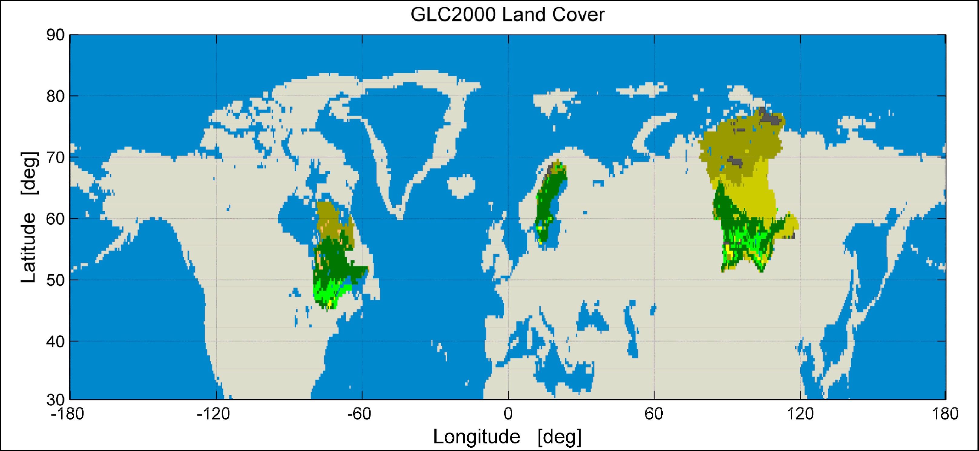
Sweden covers 450,295 km2 between 56°N and 69°N, and 10°E and 24°E. Forest is the predominant land cover (55%), with wetlands, grassland, arable land, and water bodies representing other major land cover classes [40] (Figure 1). Topography is mostly flat to moderately flat; in the northwest, mountain ridges run along the border with Norway. Forests are primarily boreal and hemi-boreal coniferous species (Norway spruce and Scotch pine). Birch is the main deciduous tree species. Forest cover, growth, and GSV are strongly related to climate. The GSV is highest at the southern latitudes, corresponding to the transition from boreal to hemi-boreal forests. Above 60°N, GSV is higher along the coast as compared to inland.
2.2. Central Siberia
Central Siberia is a 3.28 million km2 region between 52°N and 72°N, and 88°E and 110°E, containing the Krasnoyarsk Kray and the Irkutsk Oblast administrative regions. These regions include almost all vegetation zones located within the northern hemisphere with forested areas corresponding to the predominant land cover (59% in Krasnoyarsk Kray and 82% in Irkutsk Oblast) [41] (Figure 1). The remaining land cover classes consist of pasture/grassland, agriculture in the southern plains, wetlands, water bodies, and urban settlements. The topography in these regions ranges from mostly flat to moderately hilly. The southernmost part of the region includes the Sayan Mountains range, with elevations between 2,000 m and 2,700 m and areas of steep slopes. The study region is completely within the boreal zone with the exception of a relatively narrow polar belt along the Arctic shoreline. Forest cover, growth, and GSV decrease with increasing latitude. At the northernmost latitudes, the land cover consists primarily of tundra vegetation, which changes naturally from Arctic tundra to shrubland and forest tundra. South of the tundra zone, the dominant forest species is larch. Towards the south, conifers (mostly pine, spruce, fir, and Siberian cedar) represent the mature stage of forests, whereas young forests are mostly characterized by deciduous pioneer species such as birch and aspen. This is a result of natural regeneration following forest disturbance or natural succession, which has a rotation of about 70–100 years.
2.3. Québec
The province of Québec in eastern Canada covers 1,667,441 km2 between 45°N and 63°N, and −80°E and −57°E. Nearly half of the area is covered by forests representing about 20% of all forested lands in Canada (Figure 1, [42]). The topography is mostly flat with some gently rolling hills and steep-sided low altitude mountains in localized regions. Numerous water bodies occupy more than 20% of the territory. The forests of Québec belong to three major vegetation zones that fall predominantly into the Boreal Shield and Taiga Shield described by the terrestrial ecozones of Canada [43]. The southern region is characterized by deciduous and mixed temperate forests dominated by maple, yellow birch, and balsam fir with the largest GSV found in Québec. The large central region in the southern half includes dense boreal forests composed mainly of black spruce, balsam fir, and white birch, whereas the northern half corresponds to the large boreal/taiga/tundra south/north transition zone dominated by increasingly sparse and fragmented black spruce forests. The northern region includes tundra dominated by shrubland.
3. Material and Methods
This Section provides an overview of (i) the SAR datasets, (ii) the BIOMASAR algorithm used to estimate GSV from the SAR data, (iii) the datasets used for validating or comparing the SAR-based GSV estimates and assessing the reliability of SAR-based GSV, and (iv) the approach followed for the inter-comparison.
3.1. SAR Datasets
The SAR datasets consisted of images of the radar backscatter acquired by Envisat ASAR in ScanSAR mode. This imaging mode covered a swath of approximately 400 km, which in turn implied a high frequency of observations because of the large overlap of adjacent swaths. At 60°N, measurements were possible on a daily basis. Depending on the sampling bit rate, the image products were characterized by a spatial resolution of approximately 150 m (Wide Swath Mode, WSM) or 1,000 m (Global Monitoring Mode, GMM) [32]. Data are provided to the user by the European Space Agency (ESA), slightly oversampled (75 m for WSM and 500 m for GMM). GMM data were acquired regularly, whereas WSM data were acquired either upon request or according to strategic planning by ESA. In ScanSAR mode, ASAR acquired either (transmit-receive) Horizontal-Horizontal, HH, or Vertical-Vertical, VV, polarized data.
For each study region, all GMM images acquired between December 2004 and February 2006, were used. For South Sweden, all WSM images acquired during the same time period were also used because of relatively poor coverage in GMM. The time interval maximized the number of winter-time images in the SAR backscatter time series, which were found to be most suitable for retrieving GSV [36]. The average and the standard deviation of the number of backscatter measurements are listed in Table 1 for each study region. The slightly larger standard deviation in Québec is a result of substantially less acquisitions south of 50°N. At least 50 backscatter measurements per pixel were available over forested areas which was found to be sufficient to obtain a reliable spatial representation of the GSV patterns [36]. To the best of our knowledge, no significant disturbance occurred within the time span of the SAR datasets. The dataset consisted of images acquired in HH- and VV-polarizations.
3.2. BIOMASAR Algorithm
The BIOMASAR algorithm [36] consists of (i) a SAR processing block to obtain calibrated, geocoded and co-registered images of the radar backscatter, and (ii) a GSV retrieval block where each of the radar backscatter measurements is inverted to GSV by means of a semi-empirical forest backscatter model and individual GSV estimates are blended with a weighted linear combination to form the final estimate of GSV. A summary of the main components of the algorithm and details about the implementation for this study are given below. Further information regarding the development and validation of the BIOMASAR algorithm has been reported in [36].
3.2.1. SAR Processing
The SAR data were obtained in the form of image strips of backscattered intensity in the geometry of acquisition of the radar sensor. Each data strip was multi-looked (i.e., boxcar averaged) to reduce speckle noise. As a trade-off between spatial resolution and speckle noise reduction, the data were multi-looked to form pixels with a size of 1,000 m. Each strip was then terrain geocoded [44] to the equiangular projection and to the pixel size of 0.01°. Terrain information was available from Digital Elevation Models (DEMs) [45–47]. The resulting geocoding accuracy was on the order of 1/3 of the pixel size. The SAR backscatter was then corrected for the pixel area determined from the DEM [48]. The SAR images were subsequently tiled according to a regular 2° × 2° grid for optimal management of computing resources. To further mitigate speckle noise, each set of images within a tile was filtered with a multi-channel approach [49]. The estimated Equivalent Number of Looks (ENL) [50] was close to 60 in the case of a GMM dataset with approximately 100 measurements or a WSM dataset. For GMM datasets with less than 50 observations, the ENL was close to 40. The corresponding uncertainty of the measured backscatter was 0.4 dB and 0.5 dB, respectively. Although such an uncertainty can play a significant role on the single image retrieval because of the exponential type of model used for the retrieval (see Section 3.2.2), the impact on the multi-temporal retrieval is much weaker because of the large number of images that are combined. In [36], the average uncertainty related to the retrieval approach was on average 10%.
3.2.2. Forest Backscatter Model and Estimation of Model Parameters
The retrieval was based on a Water Cloud type of model linking the forest GSV, V, in m3/ha to the forest backscatter coefficient, σ0for, in linear scale [33,36,51,52]. This modeling solution allows for a complete characterization of the backscattered intensity from a forest at C-band in terms of its main contributions with a simple formulation.
In Equation (1), the forest backscatter is expressed as a contribution from the ground with a backscatter coefficient of σ0gr, and from the vegetation layer with a backscatter coefficient of σ0veg, both expressed in the linear scale. The backscatter coefficients are influenced by the environmental conditions at the time of image acquisition as well as by look geometry and polarization. Nonetheless, at coarse spatial resolution, the environmental conditions are mostly affecting the backscatter coefficients [38]. Both contributions are weighted by the forest transmissivity expressed as e−βV, where β is an empirically defined coefficient (unit: ha/m3). Higher order scattering contributions (double and multiple bounces) are not included as shown to be of minor importance at C-band in boreal forest [51,53].
The two backscatter coefficients σ0gr and σ0veg and the coefficient β are unknown. In [36], we concluded that using a constant value for the latter (0.006 ha/m3) affected the retrieval only marginally when compared to a more rigorous estimate, which would require knowledge of local environmental conditions (i.e., weather data) as the transmissivity depends on the dielectric properties of the canopy and the amount of gaps within it. As the SAR backscatter at C-band is characterized by significant spatial variability as a consequence of the strong effect of environmental conditions, the two remaining unknown model parameters were estimated on a pixel-by-pixel basis.
The backscatter coefficient σ0gr was estimated by means of an automated procedure involving the computation of the mean value of the measured backscatter for pixels that can be labeled as “unvegetated” within a window centered on the pixel of interest [36]. The mask supporting the selection of backscatter measurements corresponding to unvegetated pixels was based on the MODIS Vegetation Continuous Field (VCF) tree cover product [54]. An adaptive threshold for the upper tree cover percentage and an adaptive window size were used [36].
The backscatter coefficient σ0veg was obtained in a similar manner using measurements of the backscatter coefficient corresponding to pixels labeled as “dense forest”. Dense forests were identified using the MODIS VCF product based on a minimum threshold on tree cover percentage [36]. Threshold and window size were adaptive. The mean value of the backscatter coefficient of “dense forest”, referred to as σ0df, was then compensated for the proportion of ground contribution to obtain the effective backscatter coefficient of the vegetation layer σ0veg. The compensation term was derived from Equation (1) by expressing the backscatter coefficient σ0veg as a function of the measured forest backscatter coefficient of dense forest and the modeled ground contribution.
In Equation (2), Vdf represents the GSV value assumed to be representative for “dense forest”. By definition, Vdf corresponds to the 90th percentile of the GSV distribution in the area of interest [36]. In support of the definition, knowledge of the cumulative distribution function (cdf) of GSV within the sampling unit of the parameter is required. In the case where the cdf is unknown, the value is estimated depending on which parameters of the cdf are available or can be derived, for example, from the literature. It was here assumed that a single value is representative for a 2° × 2° tile. To obtain a smooth variation of the parameter between adjacent tiles, the individual values were interpolated using a bilinear function. The parameter Vdf was also used to set the maximum GSV that can be retrieved [36]. As a consequence, erroneous values of Vdf could bias the retrieved GSV. In the case of biases greater than 20% over several adjacent tiles, fine-tuning of Vdf was applied. The presence of biases was assessed by comparing aggregated ASAR GSV and GSV of a reference dataset (see Table 2) at the very coarse resolution of 2°.
3.2.3. GSV Retrieval and Multi-Temporal Combination of GSV Estimates
For a measurement of the forest backscatter coefficient σ0for, the forest backscatter model in Equation (1) is inverted to retrieve GSV using the corresponding estimates of σ0gr and σ0veg.
The individual GSV estimates, Vi, are finally used in a weighted linear combination to form the multi-temporal estimate of GSV [35].
In Equation (4), the multi-temporal estimate of GSV, Vmt, expresses the sum of the individual GSV estimates Vi weighted by the backscatter difference between vegetation and ground (wi = σ0veg − σ0gr, in the dB scale). The coefficient wmax is equal to the largest of the weights wi. Such weighting approach maximizes the contribution of GSV estimates from images characterized by a large contrast between forest and non-forest backscatter and avoids that images with little backscatter variability between low and high GSV can distort the final GSV estimate [36]. N represents the number of estimates being combined. Estimates corresponding to wi below 0.5 were discarded because likely to be uncertain [36].
In this study, GSV estimates were obtained at 0.01°. In addition, spatial averaging was applied to derive estimates at coarser spatial resolution. Our interest was primarily to derive estimates for spatial resolutions commonly used in carbon and biosphere models (0.1° and 0.5°).
3.3. GSV Datasets
Three types of GSV datasets were used in this study to assess the accuracy and the reliability of GSV estimated with the BIOMASAR algorithm from the ASAR datasets: forest field inventory datasets, spatially explicit estimates obtained from Earth Observation (EO) data, and global estimates of GSV or carbon stocks obtained from multiple input sources.
Forest field inventory datasets qualify as validation datasets. Nonetheless, if the scale of the forest field inventory data does not match the scale of the EO data, the characterization of GSV in each of the datasets is different. Therefore, they are of limited usefulness to derive correct information on the retrieval accuracy of GSV from the remote sensing data. In this study, we considered several datasets based on forest field inventory measurements at multiple scales to finally assess the impact of scales on the GSV retrieval.
Estimates of GSV from forest field measurements are often used in combination with EO satellite imagery to provide spatially explicit estimates of GSV. This procedure is implemented by several national forest inventories, for example in Sweden and Canada. The accuracy of the estimates of the forest variable of interest can be low at the pixel level whereas with aggregation of adjacent pixels, increased accuracy can be achieved [10,55]. In this study, we considered EO-based GSV raster datasets that are produced by, or in support of, national forest inventories and therefore assumed to be sufficiently reliable to identify inconsistencies in the ASAR GSV estimates.
Global maps of GSV (or alternatively carbon stocks) derived from a combination of multiple data sources (in situ measurements, administrative statistics, model predictions, and remote sensing datasets) were considered as they cover all regions and, thus, allow comparison of results among them with a common basis. Although such datasets can only be considered for comparison purposes as they do not qualify as reference sets for validation, they were of interest to benchmark the ASAR GSV and assess its overall reliability towards quantifying forest resources and carbon stocks in the boreal zone and to pinpoint areas of discrepancy.
Table 2 provides an overview of the three different types of GSV datasets for the three study regions ([6,7,10,29,39,55–57]). If necessary, datasets were re-projected and resampled into the geographic projection used for the ASAR data. Further details about each dataset are provided in related Sections below.
3.3.1. Forest Field Inventory Datasets
Plot-wise measurements of GSV from the Swedish National Forest Inventory (NFI) were available for the entire country (Table 2). The Swedish NFI data consisted of GSV measured within plots of 7 m or 10 m radius, located on a pre-defined grid throughout the country [7]. For this study, the GSV from NFI plots field inventoried between 2004 and 2006 were averaged using 1 km × 1 km grid cells to form estimates at the same spatial scale as the estimates of ASAR GSV. In total, 11,425 GSV estimates were obtained. The number of recruited inventory plots within an ASAR pixel ranged from 1 to 13 with 90% of the 1 km estimates based on less than 4 plots.
For Central Siberia, a first dataset consisted of forest field inventory data arranged to form polygon-wise measurements of GSV. A polygon corresponds to an area with similar forest properties in terms of tree species, age, productivity, GSV and local homogeneity. Such data were available from ten forest enterprises located in Irkutsk Oblast [29] (Tables 2 and 3) and originated from forest surveys carried out according to the Russian Forest Inventory Manual [58]. Forest stand boundaries were based on manual interpretation of aerial photographs. The dataset was last inventoried in 1998, with updates to 2003 to reflect forest cover changes. While the error of the field inventory data was within requirements to not exceed 15% of GSV of the Forest Inventory, measurements in dense forest were systematically underestimated by approximately 10% [59]. Accordingly, a correction factor was applied. To take into account the 7-year time difference between the field inventory and the acquisition of the ASAR data, yearly growth factors were applied [36]. This corresponded to a yearly increase of productivity in the taiga forest over the recent decades of 0.3–0.5% per year [60]. For the inter-comparison, the data were rasterized to 100 m, averaged to 1 km and resampled to 0.01° pixel size.
A second dataset was a regional vegetation database covering the entire study region [39] (Tables 2 and 3). The polygons of the vegetation database were delineated by Russian regional forest inventory and vegetation experts using aerial photographs. Although the polygons were defined in terms of broad homogeneous forest cover, occasionally they could include very different forest cover conditions on relatively small areas (e.g., harvested forest and dense mature forest), which are not accounted for by field measurements. Due to the vastness of the area and the remoteness of large parts of the region, the field inventory data had different levels of accuracy and currency. The majority of the data in the vegetation database stemmed from inventories undertaken at the end of the 1990s. For some areas in the north of the study region, the initial inventory data were 20–30 years old. For the southernmost regions, availability of recent aerial photography and satellite images allowed for correction of obsolete values. Exact information on the year of inventory and accuracy of the data were not available for updating of the GSV data as in the case of the forest enterprises. Despite several caveats, this dataset provided the most comprehensive information on GSV at the time of acquisition of the ASAR images for the entire study region.
3.3.2. Earth Observation Raster Datasets
Spatially explicit estimates of GSV for Sweden with a pixel size of 25 m were obtained for the year 2005 from a combination of optical satellite remote sensing data and NFI data, and through applying the k-Nearest Neighbor (kNN) algorithm (Table 2) [61]. For a similar product created with data from the year 2000, the relative Root Mean Square Error (RMSE) of the GSV estimates was below 20% when aggregating over areas larger than 1 km2 [10]. In this study, the 25 m GSV values were aggregated to 1 km, assuming that the result would correspond to the estimates by kNN at the scale of the ASAR data.
A sample set of forest volume density (m3/ha) representative for Québec was extracted from the Earth Observation for Sustainable Development (EOSD) map product (Table 2). The EOSD project was established to create a 23-class land cover map of the forested areas of Canada from approximately the year 2000 [62], as well as related total volume and biomass maps [55]. Inventory-based models were used to assign total volume and biomass estimates to EOSD forest land cover classes through a process involving ecozone stratification, climate, stand height imputation, and reference to stand age in Canada’s National Forest Inventory [9,55]. These EO-based maps were produced for the forested areas of Canada and used to provide total volume and biomass estimates for the Canadian NFI [9], mostly in Northern Canada over regions where traditional inventory data were not available from provincial and territorial sources. Full-resolution estimates were aggregated to various scales for validation purposes and the optimal cell size was found to be 100 km2 in size with a coefficient of determination (R2) of 0.8 and RMSEs that ranged from 7 tons/ha to 57 tons/ha for biomass [55]. Despite this large cell size, aggregation at 1 km resolution was found to provide sufficiently reliable estimates for comparison purpose. All 1 km resolution EOSD total volume map pixels located on the Canadian NFI systematic grid and fully comprised within 2 km × 2 km NFI photo-plots which had not experienced change as a result of natural or anthropogenic disturbance, between 2000 and 2005, were selected across all forested regions of Québec, yielding a total of 731 samples.
3.3.3. Global GSV and Carbon Stocks Datasets
The International Institute for Applied Systems Analysis (IIASA) dataset of global GSV consists of spatially explicit estimates at a resolution of 0.5° (Table 2) [6]. The estimates of GSV were extrapolated from country-level GSV statistics reported in the Food and Agriculture Organization (FAO) Forest Resource Assessments 2005 to a 0.5° grid with the aid of a global 0.5° map of Net Primary Productivity (NPP) and maps indicating the human influence. The quality of the estimates was reported to differ depending on the reliability of the input forest data provided by the individual nations.
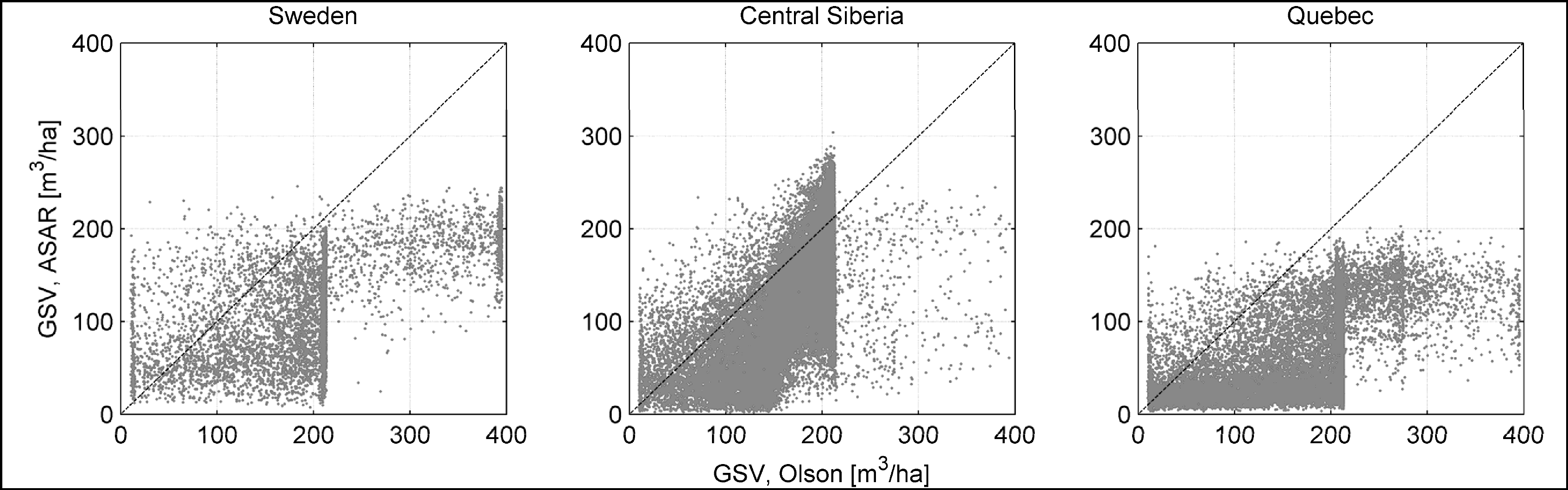
The updated Olson database of carbon stocks [56] and the Ruesch & Gibbs dataset of carbon stocks [57] provide estimates of carbon stocks in vegetation on a global scale (Table 2). The former dataset is based on vegetation information in the original Olson database [63] updated with land cover information from the Global Land Cover product GLC2000 [42]. The latter dataset is based on default biome-wise mean values of carbon stocks compiled by the Intergovernmental Panel on Climate Change (IPCC) for the major ecozones of the world and extrapolated to the forest area of the particular country. The datasets have a pixel size of 0.089° and 0.0083°, respectively.
To convert carbon stock values to GSV, Equation (5) was used [64]. The Biomass Conversion and Expansion Factor (BCEF) allows converting between GSV and above-ground biomass. The Root-to-Shoot ratio (RS) expresses the relation between above- and below-ground biomass. The Carbon Fraction (CF) indicates the carbon fraction of forest biomass.
It was preferred to convert carbon stocks into GSV rather than vice versa, since the level of detail in the global carbon stocks datasets was lower compared to the GSV datasets. In this way, we tried to minimize the effect of the conversion on the interpretation of the comparison between the different products. As BCEF depended on vegetation type, the GLC2000 land cover map was used to support the correct attribution of a value of BCEF to each pixel within the study regions. The dependency of BCEF upon volume classes was neglected since the differences in the boreal zone are minimal.
3.4. Statistical Measures for Assessment of GSV Retrieval
The GSV retrieved from the ASAR data was compared against the individual GSV datasets described in Table 2 by means of scatterplots and agreement statistics at 0.01°, 0.1°, and 0.5° pixel size. The estimates of ASAR GSV were assessed in terms of accuracy (with respect to forest field inventory or EO raster datasets) and reliability (with respect to the global datasets) by means of a set of statistical measures of agreement in a similar manner to [36]:
the Pearson’s correlation coefficient (r);
the relative Root Mean Squared Deviation (RMSD) [65] defined as the square root of the MSD, Equation (6), divided by the mean value of the GSV dataset selected as reference;
the bias, defined as the difference of the ASAR GSV and reference GSV mean values.
The MSD includes the mean values of the ASAR GSV and the GSV of the dataset against which it is compared, μASAR and μother. σ2ASAR and σ2other represent the corresponding variances whereas σASAR,other represented the covariance between the two datasets. As a measure of the relative difference between the ASAR and the reference GSV, we preferred using the RMSD instead of the more common RMSE since several reference datasets used in this study represented an estimate of GSV themselves.
4. Results
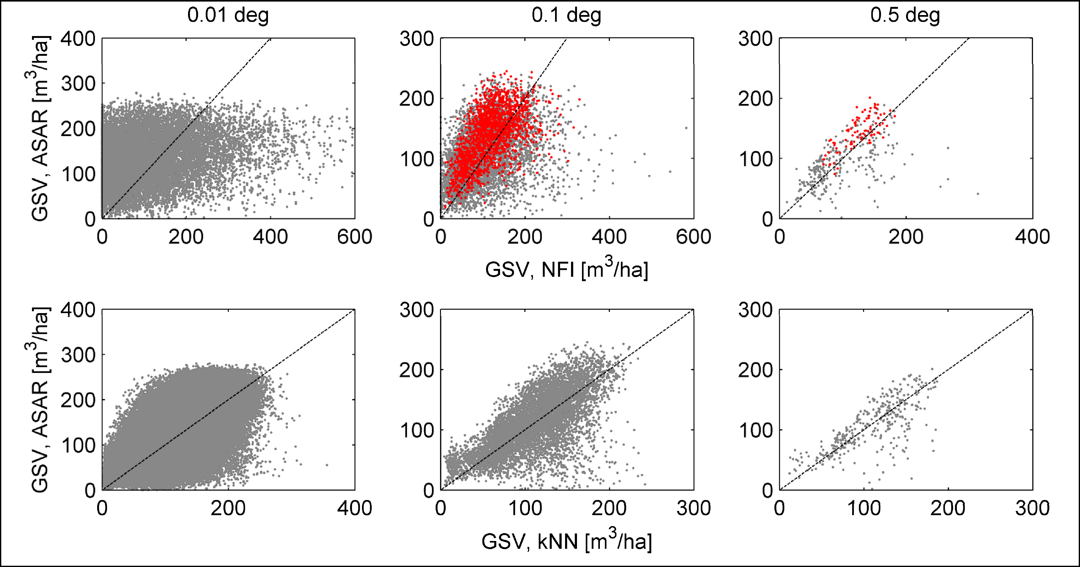
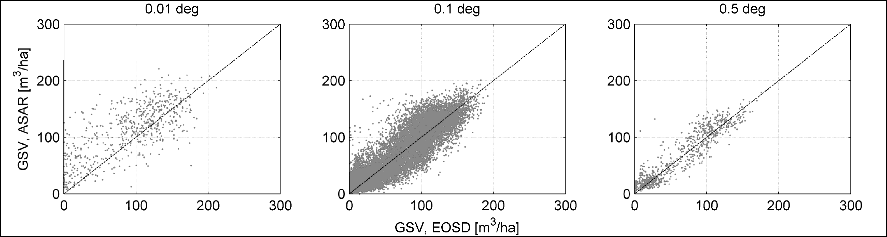
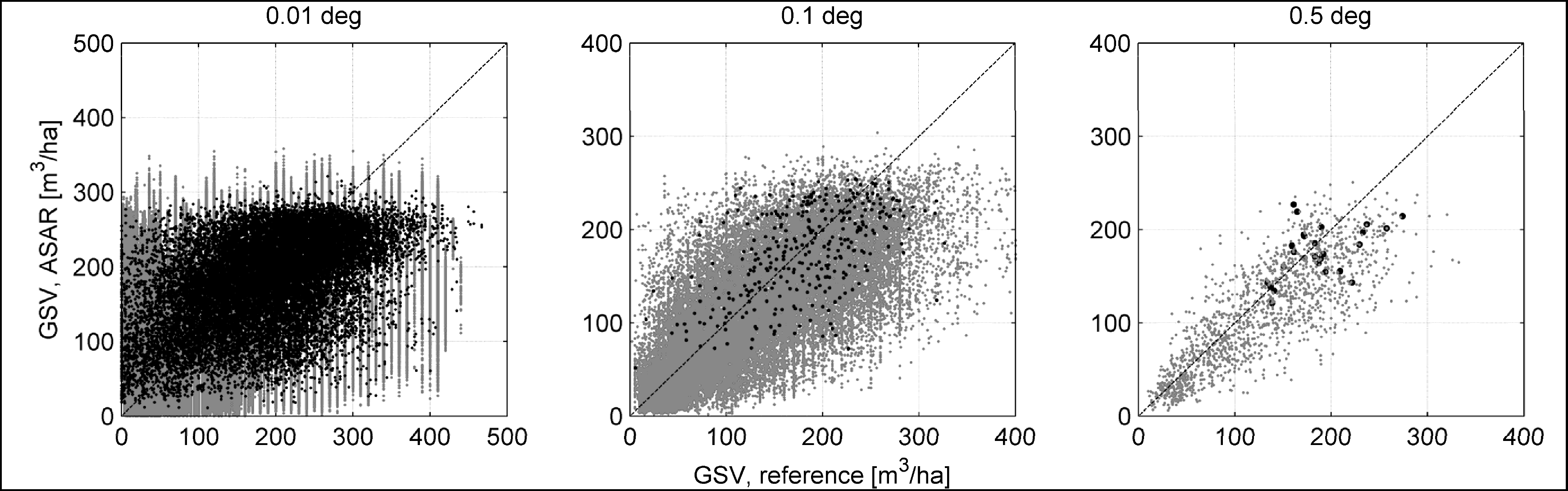
The relationships between ASAR GSV with GSV from the Swedish NFI and kNN became more pronounced for increasing pixel size with the most obvious linear association at 0.5° (Figure 2). This was supported by the relative RMSDs between ASAR and NFI or kNN, which were identical at 0.5° although bias values were smallest for kNN (Table 4). The relative RMSD values also consistently decreased as pixel size increased (Table 4). These observations were replicated in the scatterplots for Central Siberia (Figure 3) and Québec (Figure 4), and similarly for the agreement statistics as a function of pixel size with the highest correlation and smallest relative RMSD and bias at 0.5° for Central Siberia and Québec (Table 4).
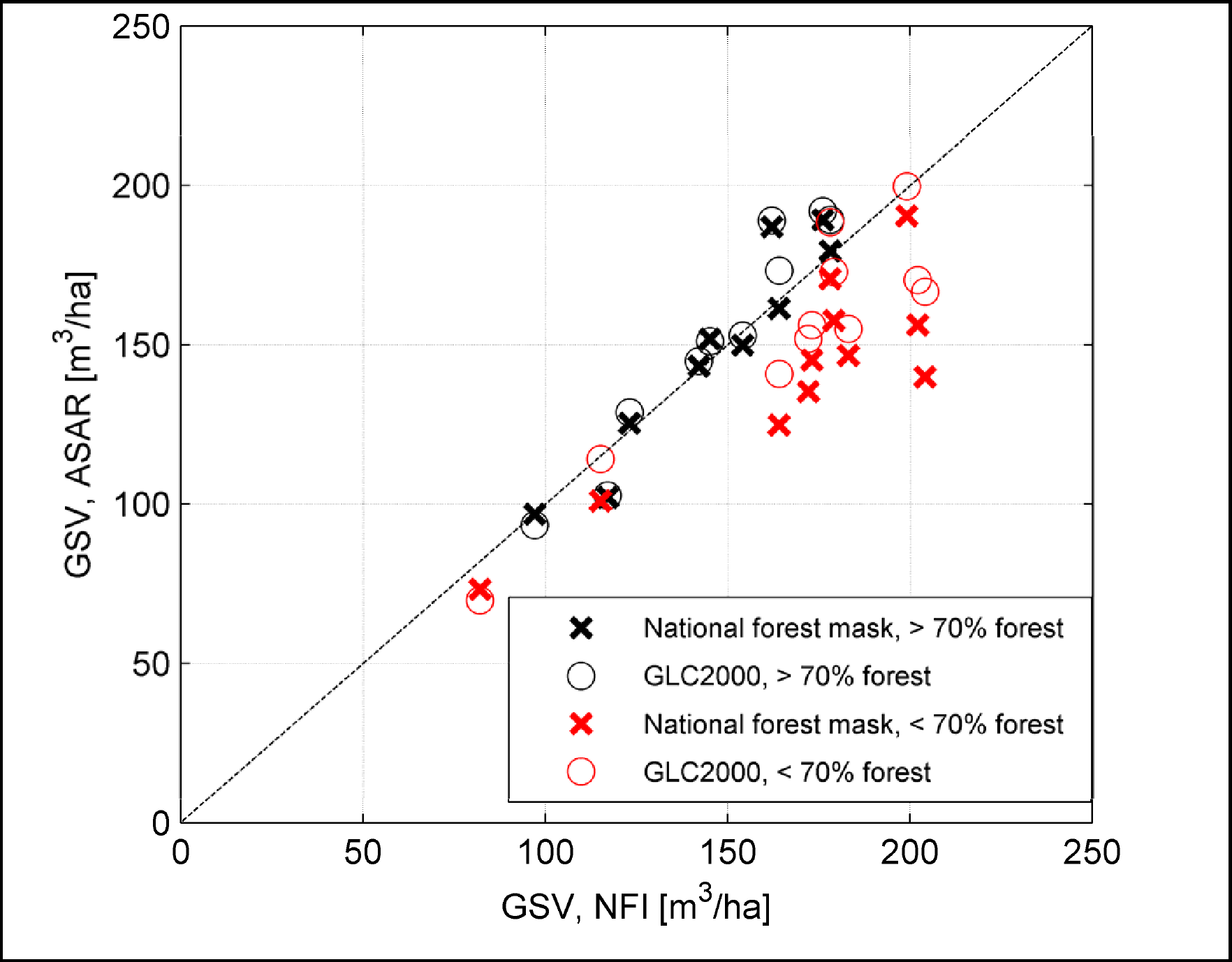
For Sweden, the agreement between ASAR GSV and NFI GSV improved when restricting the analysis to the 25% of ASAR pixels containing the largest number of NFI plots (Figure 2, top row). Nevertheless, the ASAR dataset was characterized by somewhat larger estimates. For the full dataset of NFI plots, the correlation coefficient between the datasets was always below 0.6 and the relative RMSD reached at most the 40% level (Table 4). When restricting the analysis to the 25% of pixels with the largest number of plots, the correlation reached 0.73 and the error was on the order of 20–40% depending on the level of aggregation (Table 4).
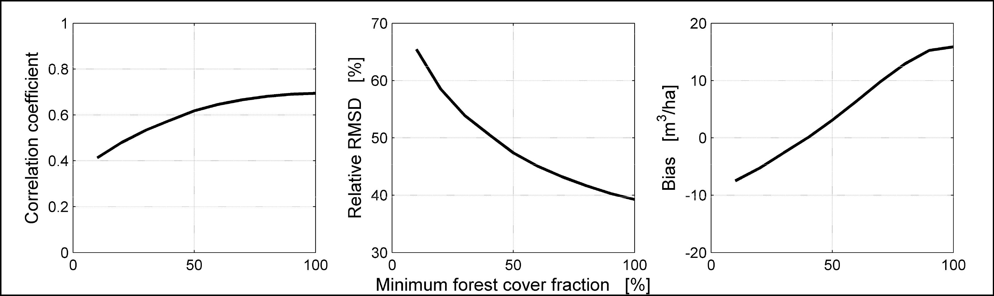
To verify the impact of land fragmentation on the retrieved GSV at kilometric scale, we computed the fraction of forest cover according to the national forest/non-forest layer also used for the kNN data product and compared to the difference between ASAR and kNN GSV. The agreement between ASAR and kNN GSV increased for increasing forest cover fraction as shown by the trends in the correlation coefficient and the relative RMSD (Figure 5) with respect to minimum forest cover fraction. The estimation bias was also affected, with substantial increase from negative to positive values.
For Sweden, average ASAR GSV was also computed at the county level and then compared to corresponding values published by the Swedish NFI [40] for the period 2004–2008 (Figure 6). The county-wise GSV values published by the NFI were reported for forested land, defined as land suitable for forest production (yearly ideal production > 1 m3/ha). Accordingly, the county-wise averages from the ASAR GSV estimates were computed for pixels belonging to the forest class. A forest/non-forest mask was derived from the kNN dataset, which is based on the definition of the Swedish NFI. In addition, we also considered a forest/non-forest mask derived from the global GLC2000 land-cover dataset. This served to verify the impact of the definition of forest land in different forest masks on the county-wise statistics. The greatest correspondence between ASAR GSV and NFI GSV occurred in areas dominated by forest cover (>70%); counties characterized by land fragmentation presented lower ASAR GSV compared to the corresponding NFI estimate (Figure 6). In such counties, the GSV estimate by ASAR was furthermore affected by the choice of the forest mask.
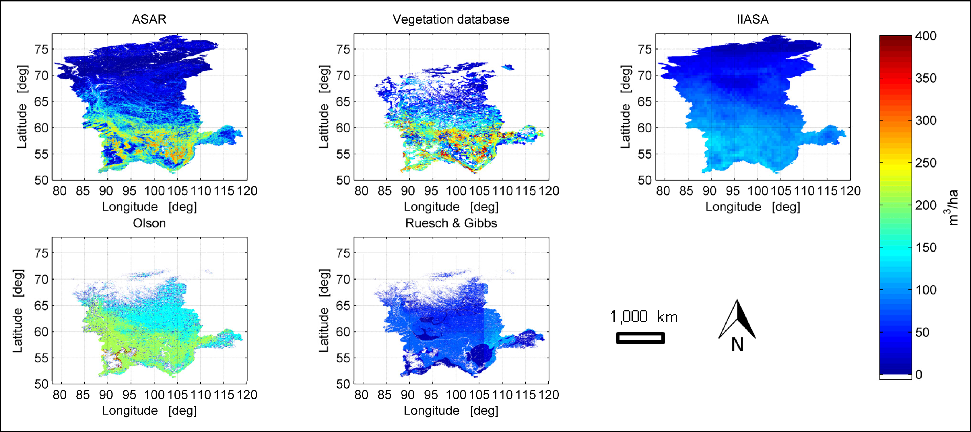
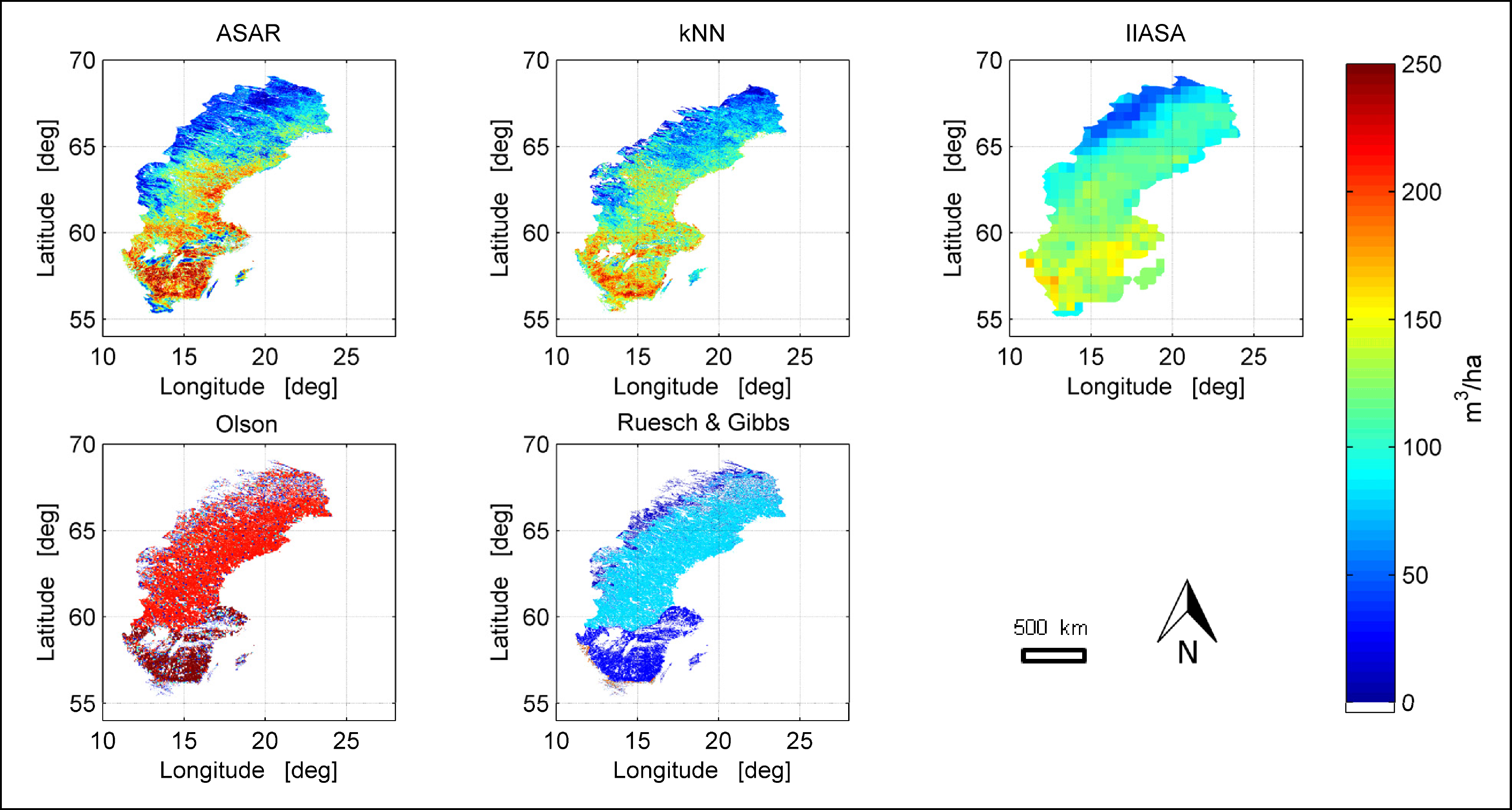
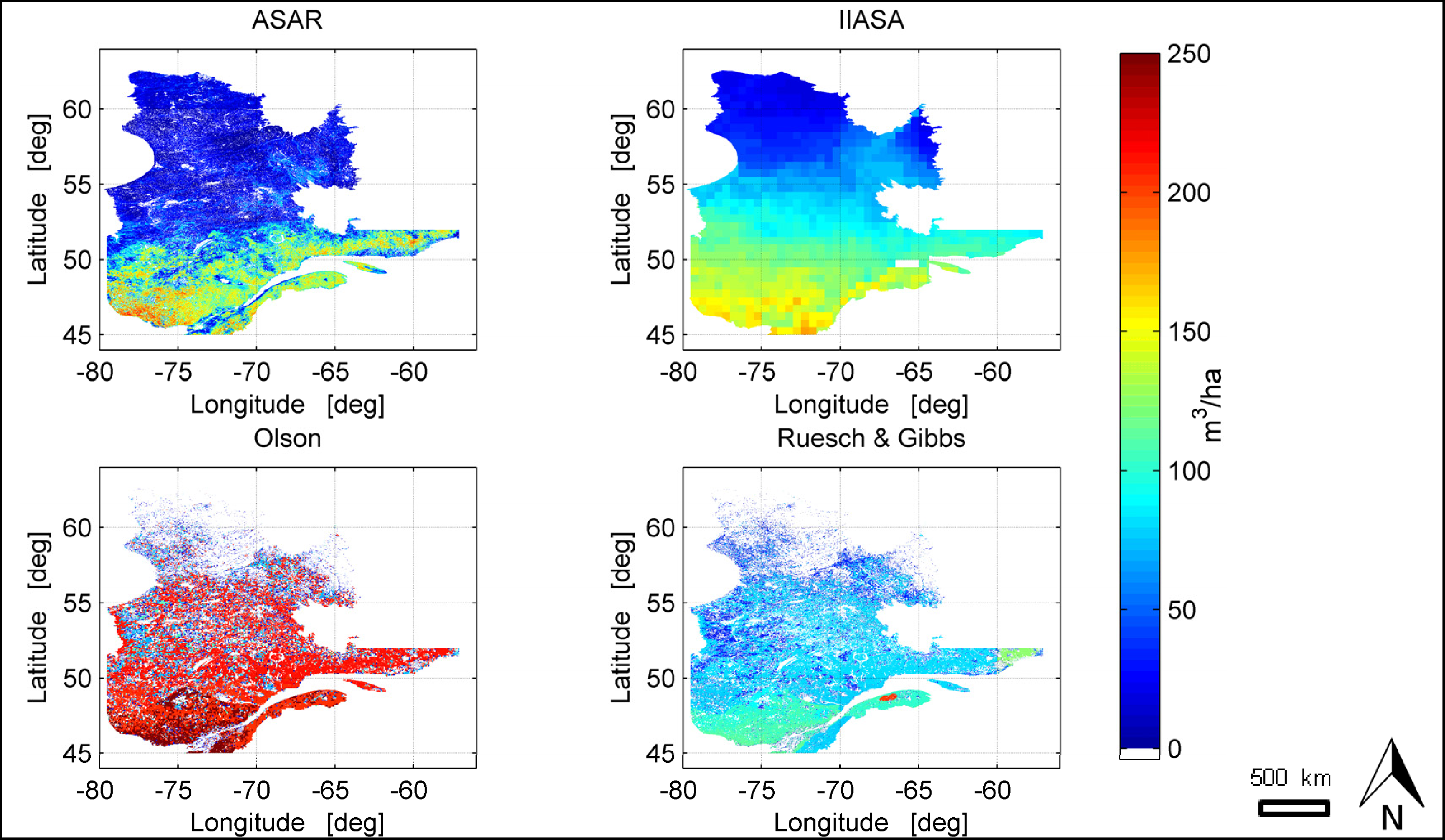
Visual observations depicted considerable variation when comparing maps of ASAR GSV with other raster GSV across each of the study regions: Sweden (Figure 7), Central Siberia (Figure 8), and Québec (Figure 9). The maps of ASAR GSV appeared to illustrate the greatest variation and thus sensitivity to differences in GSV in the ASAR GSV map compared to those derived from other raster GSV datasets.
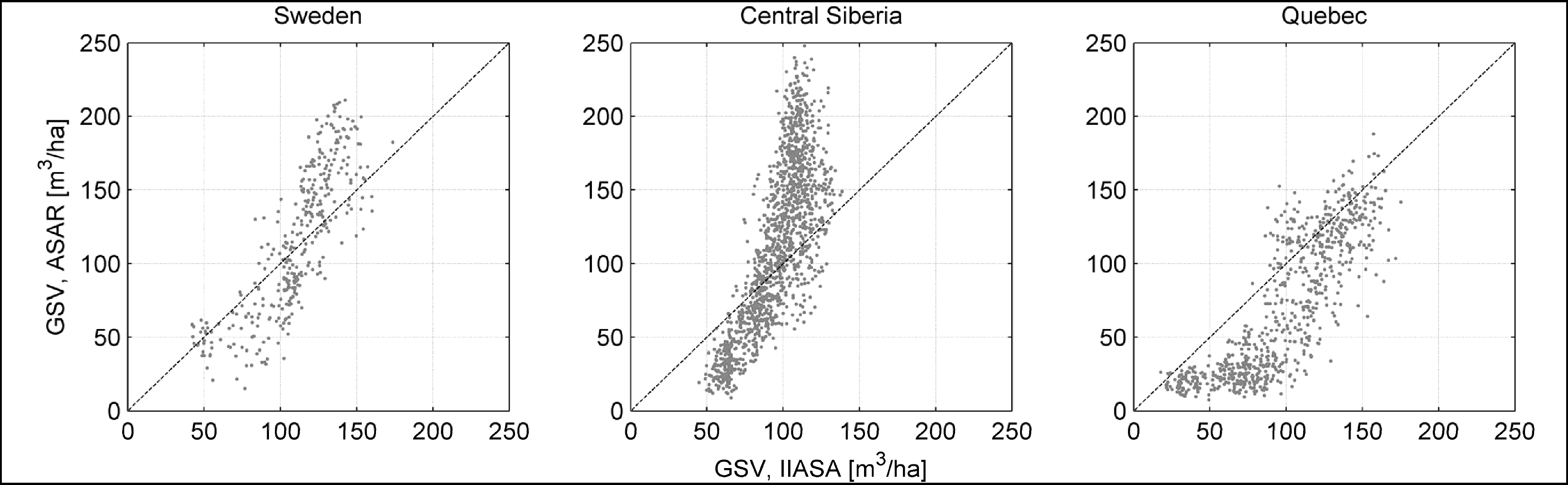
The spatial detail in the ASAR GSV estimates was by far greater compared to the representation of GSV given by the global datasets of GSV and carbon stocks. The IIASA GSV dataset presented the smoothest variability across each of the study regions and the best correspondence with the ASAR GSV (Table 5, Figure 10). The two datasets of carbon stocks provided a discrete and very coarse representation of the spatial distribution of biomass in consequence of their definition of depicting carbon at the level of ecozones (Table 5, Figures 11 and 12).
Assessing the contribution of ASAR data in terms of forest resources quantification consisted of a comparison of average GSV and total volume for the three study regions with respect to corresponding figures either published in literature (Sweden) or derived from the reference datasets (Central Siberia and Québec). For Sweden, the ASAR GSV generated the smallest average GSV whereas the total volume was largest, regardless of the forest mask used (Table 6). For Central Siberia, estimates were computed for the ten forest enterprises in the Irkutsk Oblast region and the area covered by the vegetation database (Table 3). For the former, we present the statistics for (i) the original measurements relative to 1998, (ii) the measurements of 1998 corrected for underestimation in mature forest, and (iii) the measurements updated for the year 2005. For the latter, it was not possible to correct for growth, disturbances, and intrinsic errors of the inventory. However, a comparison of resources derived from the ASAR GSV and the vegetation database was significant because the vegetation database provided the most recent update on forest GSV for the whole territory of Central Siberia. Based on this comparison, ASAR GSV values were very similar to those derived from the 1998 forest field inventory (Table 7).
A comparison across all forested regions of Québec (including non-inventoried northern regions and excluding tundra ecozones) was feasible using the EOSD 1 km GSV map whereby ASAR GSV and EOSD values were almost the same for the entire Province of Québec (Table 8). A further comparison across southern inventoried regions (merchantable forests, thus, with higher GSV values) was undertaken using a sample set from the Canadian NFI inventory (n = 658). Polygon-level GSV estimates [66] available within 2 km × 2 km NFI photo-plots [9] were aggregated at 1 km resolution. The corresponding average GSV was smallest compared to the estimates obtained from the EOSD and the ASAR datasets (Table 8). Information on total volume was not available.
5. Discussion
5.1. Multi-Scale Assessment of ASAR GSV Estimates
The agreement between the ASAR and the NFI GSV of Sweden at 0.01° pixel size was poor because of the sparse plot sampling and the large difference between the size of a NFI plot and the size of an ASAR pixel (Figure 2(top)). More meaningful was the comparison at coarser pixel size. The very detailed description of the GSV provided by one or a few neighboring NFI plots did not necessarily coincide with the GSV over a 1 km2 area. Aggregation over several NFI GSV estimates such as to form 10 km or 50 km estimates (i.e., at 0.1° and 0.5°) decreased the contribution of very local forest conditions embedded in single plot-based measurements on the resulting GSV value. Such an estimate is then closer to the type of estimate obtained from the coarse resolution ASAR data. In addition, the structure of the Swedish NFI plots is such that the prediction of GSV based on plot samples became more reliable for aggregated areas that were 10,000–100,000 ha in size [7].
The agreement between ASAR and kNN GSV was moderate at 0.01° (r = 0.69, relative RMSD = 39%, see Table 4) with an almost symmetric distribution of data points in the scatterplot along the 1:1 line (Figure 2(bottom)). The effect of aggregation to 0.1° and 0.5° pixel size was to generate estimates of GSV with less spatial variability, but also smaller uncertainties in both datasets [10,36] compared to the 0.01° level. At 0.1°, we obtained r = 0.84 and relative RMSD = 27%; at 0.5°, we obtained r = 0.91 and relative RMSD = 21%. The bias decreased only slightly from 16 m3/ha to 11 m3/ha, confirming the systematic higher GSV estimated by ASAR. A close look at the scatterplots relating the ASAR and the kNN GSV revealed that the agreement statistics were affected by (i) a few cases of substantially smaller estimates in the ASAR-based dataset, and (ii) several cases of slightly larger GSV in the ASAR-based dataset (Figure 2(middle)).
The ASAR GSV estimates were smaller as a result of correspondence with coastlines (not visible in Figure 7). The ASAR GSV expresses the GSV within the 1 km2 pixel regardless of the land cover; hence, the fraction of water in coastline pixels resulted in a smaller retrieved GSV compared to the water fraction it had been accounted for. Larger GSV estimates were encountered primarily in two regions located along the south-east coast and the center-east part of the country (see ASAR and kNN maps of GSV in Figure 7 at latitudes of 57°N and 63°N, respectively). To verify whether the larger GSV estimates were a consequence of an imperfect constraint to the range of GSV to be retrieved with the BIOMASAR algorithm, the retrieval was repeated for different values of the maximum retrievable GSV. The effect on the retrieval was negligible, indicating that the difference was not related to the algorithm but rather likely to be structural. This interpretation was further supported by the strong similarity between the kNN and the NFI GSV estimates at 0.5°. It could have been argued that the larger GSV obtained with the ASAR data had its origin in the different scales of the datasets (0.03 ha for NFI, 0.06 ha for kNN and 100 ha for ASAR). The retrieved GSV is equivalent to the GSV of a 1 km2 large cluster of trees where the individual forest components and other land cover features have been blended and considered as a forest unit as a whole. A 1 km GSV estimate derived from the NFI measurements or the kNN estimates was set to an average of individual GSV values within the 1 km window, each being representative of a small cluster of trees. To match with the definition of GSV of a 1 km ASAR pixel, the average also included non-forested, i.e., 0 m3/ha, pixels. As a consequence, the effect of different scales would then become more apparent in case of spatial heterogeneities of the land-cover, e.g., in case of fragmented landscapes of forest and other land cover types within the 1 km pixel of the ASAR imagery. Considering only areas with a small forest cover fraction within an ASAR pixel resulted in larger discrepancies between ASAR and kNN GSV (Figure 5). When restricting the analysis to pixels with a forest cover fraction greater than 90% the agreement statistics were r = 0.70, relative RMSD = 34.6% and bias = 19 m3/ha. These statistics are only slightly better compared to the values reported in Table 4 for all pixels because of the very large proportion of areas with unbroken forest cover in Sweden.
A further assessment of the impact of land fragmentation consisted of comparing county-wise average estimates of GSV from the ASAR dataset and corresponding figures reported by the Swedish NFI [40], and taking into account the percentage of forest cover reported by the Swedish NFI (Figure 6). Because the county-wise statistics are characterized by uncertainties less than 10% [7], they were considered suitable for benchmarking the corresponding ASAR GSV estimates. Counties with a forest proportion of over 70% were characterized by considerable agreement of average GSV (<5% absolute difference). The average GSV estimated from the ASAR data was smaller than the NFI estimates for most counties with a patchy landscape. Furthermore, the underestimation was stronger when the forest mask was based on the forest/non-forest layer used in the kNN dataset (referred to in Figure 6 as national forest mask) compared to the GLC2000 land cover product. This result contrasts with the Swedish NFI plot data and the kNN dataset where the ASAR GSV was often larger. We interpret the findings as a consequence of the definition of forest land. At the county level, forest area according to the Swedish NFI and the GLC2000 land cover differed between 10% and 30%, this being the case of counties presenting strong landscape fragmentation.
In Central Siberia, the size of an ASAR pixel was comparable to the size of the field inventory sample units of the ten forest enterprises. Thus, we expected less influence of scales on the inter-comparison between the ASAR and the forest field inventory GSV. For the original resolution of the ASAR data, the retrieved GSV showed large spread along the 1:1 line when compared to the field inventory GSV and a tendency to saturate at 300 m3/ha (Figure 3). The retrieval statistics for the ten forest enterprises in Irkutsk Oblast at 0.01° (r = 0.46, relative RMSD = 41%, bias = −8 m3/ha) were in line with the numbers obtained for four forest enterprises in Krasnoyarsk Kray where the retrieval algorithm had been validated (r = 0.65, relative RMSE = 34%, bias = −8 m3/ha) [36]. In contrast to the Swedish data, we could not assess the impact of the fraction of forest cover in a pixel since the field inventory data were at the same scale as the SAR data. Hence, the spread between the datasets should be primarily related to the weak sensitivity of the C-band backscatter to forest GSV, which is caused by the limited penetration of the microwave into the forest canopy. A multi-temporal combination served to reduce the impact of environmental conditions and residual speckle noise inherent in each observation on the retrieval but could not decrease the uncertainty of the estimation, which is embedded in the remote sensing measurement itself.
Aggregation of GSV estimates to 0.1° improved the agreement between the ASAR and forest field inventory datasets; nonetheless, the spread along the 1:1 line was still significant (Figure 3). With respect to the full resolution, the retrieval error decreased (relative RMSD = 24%) whereas the correlation coefficient increased to 0.60 (Table 4). At 0.5° pixel size, the field inventory dataset consisted of a handful of GSV values, being of limited usefulness for a statistical assessment of the retrieval. Although the agreement statistics indicate further improvement of the correlation coefficient and the relative RMSD between the two datasets (Table 4), the values were not statistically significant. At this scale, the inter-comparison with respect to the vegetation database was more meaningful because of the much larger extent of this dataset and because the size of the mapping units was on the order of 0.5°. The agreement statistics (r = 0.81, relative RMSD = 33%, bias = −18 m3/ha) and the scatterplot in Figure 3 indicate moderate agreement and several cases of smaller estimates by ASAR in high GSV areas. At higher resolution (0.01° and 0.1°), the agreement was poorer, which was partly a consequence of the different scales of the ASAR GSV and the GSV in the vegetation database (Figure 3). For these pixel sizes, the agreement statistics with respect to the vegetation database reported in Table 4 are not suited for drawing conclusions on the accuracy of the ASAR GSV in Central Siberia.
For Québec, the agreement between the ASAR GSV estimates and the samples of EOSD GSV estimates was moderate (Figure 4) with r = 0.72, relative RMSD = 46% and bias = 21 m3/ha at 0.01° pixel size (Table 4). Since the EOSD GSV samples stemmed from higher resolution estimates, discrepancies were further investigated by taking into account broad forest characteristics across Québec in a similar manner as done for Sweden. A bias was estimated by grouping ASAR GSV estimates and EOSD GSV estimates by Forest Proportion (FP) classes and Conifer species Proportion (CP) both derived from the EOSD land cover product (0% to 100 % by 10% bin). It was found that the bias in percentage decreased linearly with increasing FP and was below 10% for FP above 60%. A similar trend was observed as a function of CP. For the densely inhabited, cultivated, and broadleaf dominated St-Lawrence Lowlands ecoregion [43] Southern Québec (mean FP: 28%; mean CP: 13%), the largest bias was obtained. In contrast, for the heavily forested and conifer dominated Central Laurentian ecoregion [42] within the boreal shield ecozone (mean FP: 73%; mean CP: 83%), the bias was negligible. These results confirm greater performance of the method in areas of unbroken forest cover and when coniferous forest cover dominated the 0.01° pixel over which GSV was estimated using the ASAR data. They also suggest the importance of a multi-layer approach towards the understanding of the retrieved GSV in forest regions characterized by broadleaf species.
Aggregated estimates of ASAR and EOSD GSV at 0.1° and 0.5° pixel size presented very strong agreement (Figure 4) with correlation coefficients above 0.9 and relative RMSDs of approximately 30% (Table 4). The bias was negligible. These results were interpreted as a consequence of the increasingly smaller proportion of fragmented landscapes within the area covered by a pixel for increasing aggregation level.
5.2. Benchmarking ASAR GSV in the Context of Global Estimates of GSV
The ASAR GSV and the IIASA global GSV estimates presented similar features for all study regions (Figure 10). The IIASA dataset presented larger GSV estimates compared to the ASAR dataset for low GSV (i.e., below 100–150 m3/ha) and a tendency to saturate in high GSV forest. The level at which the IIASA global GSV would saturate with respect to the ASAR GSV was, however, slightly different but never above 150 m3/ha, i.e., well below the largest GSV for each region. The saturation of GSV in the IIASA dataset was interpreted as a consequence of the limited sensitivity in the relationship between NPP and GSV [67].
With respect to the two carbon stock datasets, the ASAR GSV showed clear differences that were related to how carbon was represented in each of the carbon stocks datasets (Figures 11 and 12). The GSV derived from the updated Olson database was considerably larger with respect to the ASAR GSV (Figure 11, Table 5), as well as with regard to all other datasets considered in this study. The GSV derived from the Ruesch & Gibbs dataset was mostly below 150 m3/ha, with the large majority of the estimates being smaller compared to the corresponding values in the ASAR GSV dataset (Figure 12). The agreement statistics confirmed the poor agreement between the two datasets (r between −0.01 and 0.52; relative RMSD between 60% and 147%) and the strong discrepancy (bias between 7 m3/ha and 164 m3/ha) (Table 5).
The poor agreement between the global datasets of GSV and the ASAR GSV indicates the limits of using default values to represent GSV or carbon stocks in boreal forest. Default values used in the carbon stock datasets are often based on measurements in only a few and mostly undisturbed forests, meaning that disturbance is hardly reflected in the maps. When accounted for, as for example in the Ruesch & Gibbs and the IIASA datasets, the influence of disturbance was taken into consideration by using maps indicating anthropogenic effects. However, these maps can be far off from the true conditions. A clear example is seen for southern Sweden in the Ruesch & Gibbs dataset (Figure 7). The Ruesch & Gibbs map shows very low carbon stocks because the South of Sweden is represented as an area with strong anthropogenic influence in the map indicating human influence. The updated Olson database instead reports the highest carbon stocks in the south with values higher than in the ASAR GSV map. This is probably due to the fact that disturbance was not considered, as the default values used in the updated Olson database refer to undisturbed forest. These results are in line with indications provided by spatially explicit maps derived from C-band interferometric SAR data, which better reflected the impact of disturbances compared to carbon stock estimates from Dynamic Global Vegetation Models (DGVM) where disturbance was considered only through long-term statistics and in an incomplete manner [68].
5.3. Quantification of Forest GSV at Regional Scale
For Sweden, the nation-wide average derived from the ASAR GSV dataset was slightly smaller than the value published by the Swedish NFI. The NFI estimated an average of 133 m3/ha based on forest field inventory data collected between 2004 and 2008 [40]. The average of ASAR GSV was 125 m3/ha when using the national forest/non-forest dataset to select pixels belonging to forest land and 132 m3/ha when selecting forest pixels on the basis of the GLC2000 land cover product (Table 6). The figures of total volume predicted from the ASAR data and by the NFI differed by about 30% (Table 6). This was consistent with the difference of total forest area between the forest/non-forest mask and the GLC2000 land cover dataset on one hand and the figure provided by the Swedish NFI.
For the ten forest compartments in Central Siberia, the average GSV and the total volume obtained from the ASAR dataset was in line with the values derived from the forest field inventory dataset if no corrections had been applied for growth and underestimation in dense forest (Table 7). Correcting for underestimation of GSV in dense forest and then also for growth implied higher average GSV and total volume. The difference between the ASAR and the field inventory GSV estimates was −4% and −13%, respectively. It is likely that these figures, in particular the latter, are somewhat biased since the inventory dataset was not updated for forest disturbances after 2003 so that in practice the forest was just allowed to grow for the last two years, while volume losses were not accounted for. However, we did not have further information to support this assumption. In addition, the yearly growth factor did not take into account specific ecological conditions of the area. The interpretation of the latter statistic should be handled carefully.
For the whole region of Central Siberia, the average GSV and the total volume estimated with the ASAR dataset was approximately 10% less compared to the figures obtained from the vegetation database (Table 7). The GSV difference between the ASAR dataset and the vegetation database revealed a considerable number of land patches characterized by negative differences. In the southern part of the study region, the ASAR GSV estimates were in many cases larger than the value reported in the vegetation database (Figure 8). Patches corresponding to smaller GSV estimates in the ASAR dataset were assumed to be due to disturbances that occurred between the time of the field survey and the acquisition of the ASAR images. The spatial consistency of the GSV differences let us conclude that the smaller ASAR GSV corresponded to forest affected by disturbance. Assessing the plausibility of this interpretation requires the availability of a pool of additional datasets related to type and extent of disturbances, which was beyond the scope of this paper.
For the Canadian NFI plots in Québec, the average GSV and the total volume from the ASAR dataset and the EOSD dataset were almost identical. With respect to these, there was an approximate 30% difference in average GSV between the Canadian NFI samples and that derived from EOSD and ASAR (Table 8). The GSV values over the inventoried portion of Québec is largely derived from provincial inventory data and likely more representative of what may exist at these locations than those derived from coarser resolution datasets used in the estimation for EOSD or from ASAR. This would imply that ASAR and EOSD GSV values may be conservative relative to what provincial inventory data used in the Canadian NFI may indicate.
6. Conclusions
Forest growing stock volume (GSV) has been estimated for three regions in the boreal zone (Sweden, Central Siberia and Québec) using the BIOMASAR approach and hyper-temporal datasets of the radar backscattered intensity acquired by Envisat ASAR in ScanSAR mode. In total, 5.3·106 km2 have been mapped to provide spatially explicit estimates of GSV with a pixel size of 0.01°, corresponding to the 1 km spatial resolution of the ASAR data. From these, aggregated values at 0.1° and 0.5° pixel size have been derived. Assessment of the 0.01° retrieved GSV with respect to forest field inventory data at similar scale indicated decent performance of the retrieval approach based on hyper-temporal C-band SAR backscatter data in boreal forest. Nonetheless, the weak sensitivity of the backscattered intensity to forest structural parameters introduced significant uncertainty to the estimated GSV. The assessment furthermore indicated the intrinsic difficulty of comparing the GSV estimates derived at coarse resolution with other datasets of GSV characterized by a much higher native spatial resolution. The scales difference revealed particularly in the case of fragmented landscapes. Here, the ASAR GSV estimates were more often in disagreement with the GSV of a reference dataset when compared to areas of predominant forest cover. Another result that was consistent among all study regions was an improved agreement between ASAR GSV and reference GSV after aggregation to coarser scales. The relative difference at 0.5° pixel size was consistently on the order of 20–30%.
Despite the weaknesses of C-band SAR backscatter to retrieve GSV, the results presented in this paper reveal the capability of a single approach to provide consistent estimates of GSV across the boreal zone and a reliable representation of the spatial distribution of GSV, improving knowledge with respect to information currently available for boreal forests. The kilometric resolution of the GSV estimates and the uncertainty associated with these estimates can be considered limiting factors where spatial detail or high estimation precision is required. Nonetheless, for regions where the GSV is poorly quantified or has not been updated in recent times, estimates provided by Envisat ASAR ScanSAR backscatter images can represent a reference dataset (e.g., as part of the federal component of the Russian forest inventory that is currently under development). Such estimates are already sufficient for integration into carbon/biosphere models. Carbon models do not require the highest possible resolution (1 km) but rather a gap-free and consistent description of the spatial distribution of biomass with 0.1° to 0.5° pixel size, which could be based on higher resolution 1 km SAR data. The availability of extensive datasets of Envisat ASAR ScanSAR data, between 2003 and 2012, at global scale, generate new possibilities for detailed assessment of the state of forests in polar and boreal domains for the last decade.
Acknowledgments
This study has been supported by ESA Support to Science Element (STSE) ESRIN contract No. 21892/08/I-EC. M. Engdahl and D. Fernandez Prieto, ESA, are acknowledged for support and scientific advice. J. Dahlgren, M. Egberth and M. Högström, Swedish University of Agricultural Sciences, are acknowledged for technical support to estimate growing stock volume from the Swedish NFI data. H. Reese, Swedish University of Agricultural Sciences, is greatly acknowledged for proof reading the manuscript. We are grateful to P. Villemare and E. Arsenault, Canadian Forest Service, for technical support. Envisat ASAR data have been acquired and distributed under ESA’s AO-225 and Category-1 project No. 6397. Collection of field inventory data for Central Siberia has been supported by the EC-funded 5th Framework Program Project SIBERIA-II (Contract No. EVG1-CT-2001-00048). The ASAR GSV datasets can be viewed at http://biomass.geo-wiki.org and are accessible at http://www.biomasar.org.
Conflict of Interest
The authors declare no conflict of interest.
References
- Houghton, R.A. Why are estimates of the terrestrial carbon balance so different? Global Change Biol 2003, 9, 500–509. [Google Scholar]
- Shvidenko, A.Z.; Schepaschenko, D.G.; Vaganov, E.A.; Nilsson, S. Net Primary Production of forest ecosystems of Russia: A new estimate. Dokl. Earth Sci 2008, 421, 1009–1012. [Google Scholar]
- Houghton, R.A.; Hall, F.; Goetz, S.J. Importance of forest biomass in the global carbon cycle. J. Geophys. Res 2009, 114, G00E03. [Google Scholar]
- Houghton, R.A. Aboveground forest biomass and the global carbon balance. Global Change Biol 2005, 11, 945–958. [Google Scholar]
- Kinnunen, J.; Maltamo, M.; Päivinen, R. Standing volume estimates of forests in Russia: How accurate is the published data? Forestry 2007, 80, 53–64. [Google Scholar]
- Kindermann, G.E.; McCallum, I.; Fritz, S.; Obersteiner, M. A global forest growing stock, biomass and carbon map based on FAO statistics. Silva Fenn 2008, 42, 387–396. [Google Scholar]
- Axelsson, A.–L.; Ståhl, G.; Söderberg, U.; Petersson, H.; Fridman, J.; Lundström, A. National Forest Inventory Reports: Sweden. In National Forest Inventories: Pathways for Common Reporting; Tomppo, E., Gschwantner, T., Lawrence, M., McRoberts, R.E., Eds.; Springer: Dordrecht, The Netherlands, 2010; pp. 541–553. [Google Scholar]
- Shvidenko, A.; Schepaschenko, D.; McCallum, I.; Nilsson, S. Can the uncertainty of full carbon accounting of forest ecosystems be made acceptable to policymakers? Clim. Change 2010, 103, 137–157. [Google Scholar]
- Gillis, M.D.; Omule, A.Y.; Brierley, T. Monitoring Canada’s forests: The National Forest Inventory. Forest. Chron 2005, 81, 214–221. [Google Scholar]
- Reese, H.; Nilsson, M.; Granqvist Pahlén, T.; Hagner, O.; Joyce, S.; Tingelöf, U.; Egberth, M.; Olsson, H. Countrywide estimates of forest variables using satellite data and field data from the National Forest Inventory. Ambio 2003, 32, 542–548. [Google Scholar]
- Houghton, R.A.; Butman, D.; Bunn, A.G.; Krankina, O.N.; Schlesinger, P.; Stone, T.A. Mapping Russian forest biomass with data from satellites and forest inventories. Environ. Res. Lett 2007, 2, 045032. [Google Scholar]
- Blackard, J.A.; Finco, M.V.; Helmer, E.H.; Holden, G.R.; Hoppus, M.L.; Jacobs, D.M.; Lister, A.J.; Moisen, G.G.; Nelson, M.D.; Riemann, R.; et al. Mapping U.S. forest biomass using nationwide forest inventory data and moderate resolution information. Remote Sens. Environ 2008, 112, 1658–1677. [Google Scholar]
- Baccini, A.; Laporte, N.; Goetz, S.J.; Sun, M.; Dong, H. A first map of tropical Africa’s above-ground biomass derived from satellite imagery. Environ. Res. Lett 2008, 3, 045011. [Google Scholar]
- Gallaun, H.; Zanchi, G.; Nabuurs, G.J.; Hengeveld, G.; Schardt, M.; Verkerk, P.J. EU–wide maps of growing stock and above-ground biomass in forests based on remote sensing and field measurements. For. Ecol. Manage 2010, 260, 252–261. [Google Scholar]
- Hansen, M.; Townshend, J.R.G.; DeFries, R.S.; Carroll, M. Estimation of tree cover using MODIS data at global, continental and regional/local scales. Int. J. Remote Sens 2005, 26, 4359–4380. [Google Scholar]
- Lefsky, M.A. A global forest canopy height map from the Moderate Resolution Imaging Spectroradiometer and the Geoscience Laser Altimeter System. Geophys. Res. Lett 2010, 37, L15401. [Google Scholar]
- Simard, M.; Pinto, N.; Fisher, J.B.; Baccini, A. Mapping forest canopy height globally with spaceborne lidar. J. Geophys. Res.-Biogeo 2011, 116, G04021. [Google Scholar]
- Boudreau, J.; Nelson, R.F.; Margolis, H.A.; Beaudoin, A.; Guindon, L.; Kimes, D.S. Regional aboveground forest biomass using airborne and spaceborne LiDAR in Québec. Remote Sens. Environ 2008, 112, 3876–3890. [Google Scholar]
- Nelson, R.; Ranson, K.J.; Sun, G.; Kimes, D.S.; Kharuk, V.; Montesano, P. Estimating Siberian timber volume using MODIS and ICESat/GLAS. Remote Sens. Environ 2009, 113, 691–701. [Google Scholar]
- Nelson, R.; Boudreau, J.; Gregoire, T.G.; Margolis, H.; Næsset, E.; Gobakken, T.; Ståhl, G. Estimating Quebec provincial forest resources using ICESat/GLAS. Can. J. For. Res 2009, 39, 862–881. [Google Scholar]
- Saatchi, S.S.; Harris, N.L.; Brown, S.; Lefsky, M.; Mitchard, E.T.A.; Salas, W.; Zutta, B.R.; Buermann, W.; Lewis, S.L.; Hagen, S.; et al. Benchmark map of forest carbon stocks in tropical regions across three continents. Proc. Natl. Acad. Sci. USA 2011, 108, 9899–9904. [Google Scholar]
- Baccini, A.; Goetz, S.J.; Walker, W.S.; Laporte, N.T.; Sun, M.; Sulla-Menashe, D.; Hackler, J.; Beck, P.S.A.; Dubayah, R.; Friedl, M.A.; et al. Estimated carbon dioxide emissions from tropical deforestation improved by carbon-density maps. Nature Climate Change 2012, 2, 182–185. [Google Scholar]
- Asner, G.P.; Powell, G.V.N.; Mascaro, J.; Knapp, D.E.; Clark, J.K.; Jacobson, J.; Kennedy-Bowdoin, T.; Balaji, A.; Paez-Acosta, G.; Victoria, E.; et al. High-resolution forest carbon stocks and emissions in the Amazon. Proc. Natl. Acad. Sci. USA 2010, 107, 16738–16742. [Google Scholar]
- Ranson, K.J.; Sun, G.; Lang, R.H.; Chauhan, N.S.; Cacciola, R.J.; Kilic, O. Mapping of boreal forest biomass from spaceborne synthetic aperture radar. J. Geophys. Res 1997, 102, 29,599–29,610. [Google Scholar]
- Saatchi, S.S.; Houghton, R.A.; Dos Santos Alvalá, R.C.; Soares, J.V.; Yu, Y. Distribution of aboveground live biomass in the Amazon basin. Global Change Biol 2007, 13, 816–837. [Google Scholar]
- Walker, W.S.; Kellndorfer, J.M.; LaPoint, E.; Hoppus, M.; Westfall, J. An empirical InSAR-optical fusion approach to mapping vegetation canopy height. Remote Sens. Environ 2007, 109, 482–499. [Google Scholar]
- Balzter, H.; Talmon, E.; Wagner, W.; Gaveau, D.; Plummer, S.; Yu, J.J.; Quegan, S.; Davidson, M.; Le Toan, T.; Gluck, M.; et al. Accuracy assessment of a large-scale forest cover map of central Siberia from synthetic aperture radar. Can. J. Remote Sens 2002, 28, 719–737. [Google Scholar]
- Gaveau, D.L.A.; Balzter, H.; Plummer, S. Forest woody biomass classification with satellite-based radar coherence over 900 000 km2 in Central Siberia. For. Ecol. Manage 2003, 174, 65–75. [Google Scholar]
- Wagner, W.; Luckman, A.; Vietmeier, J.; Tansey, K.; Balzter, H.; Schmullius, C.; Davidson, M.; Gaveau, D.; Gluck, M.; Le Toan, T.; et al. Large-scale mapping of boreal forest in SIBERIA using ERS tandem coherence and JERS backscatter data. Remote Sens. Environ 2003, 85, 125–144. [Google Scholar]
- Cartus, O.; Santoro, M.; Schmullius, C.; Li, Z. Large area forest stem volume mapping in the boreal zone using synergy of ERS-1/2 tandem coherence and MODIS vegetation continuous fields. Remote Sens. Environ 2011, 115, 931–943. [Google Scholar]
- Drezet, P.M.L.; Quegan, S. Satellite–based radar mapping of British forest age and Net Ecosystem Exchange using ERS tandem coherence. For. Ecol. Manage 2007, 238, 65–80. [Google Scholar]
- ESA. ASAR Product Handbook; ESA ESRIN: Frascati, Italy; 27; February; 2007; Issue 2.2. [Google Scholar]
- Fransson, J.E.S.; Israelsson, H. Estimation of stem volume in boreal forests using ERS-1 C- and JERS-1 L-band SAR data. Int. J. Remote Sens 1999, 20, 123–137. [Google Scholar]
- Pulliainen, J.T.; Kurvonen, L.; Hallikainen, M.T. Multitemporal behavior of L- and C-band SAR observations of boreal forests. IEEE Trans. Geosci. Remote Sens 1999, 37, 927–937. [Google Scholar]
- Santoro, M.; Askne, J.; Smith, G.; Fransson, J.E.S. Stem volume retrieval in boreal forests from ERS-1/2 interferometry. Remote Sens. Environ 2002, 81, 19–35. [Google Scholar]
- Santoro, M.; Beer, C.; Cartus, O.; Schmullius, C.; Shvidenko, A.; McCallum, I.; Wegmüller, U.; Wiesmann, A. Retrieval of growing stock volume in boreal forest using hyper-temporal series of Envisat ASAR ScanSAR backscatter measurements. Remote Sens. Environ 2011, 115, 490–507. [Google Scholar]
- Beer, C.; Lucht, W.; Schmullius, C.; Shvidenko, A. Small net carbon dioxide uptake by Russian forests during 1981–1999. Geophys. Res. Lett 2006, 33, L15403. [Google Scholar]
- Santoro, M.; Beer, C.; Shvidenko, A.; McCallum, I.; Wegmüller, U.; Wiesmann, A.; Schmullius, C. Comparison of Forest Biomass Estimates in Siberia Using Spaceborne SAR, Inventory-Based Information and the LPJ Dynamic Global Vegetation Model. Proceedings of the Envisat Symposium 2007, Montreux, France, 23–27 April 2007.
- Quegan, S.; Beer, C.; Shvidenko, A.; McCallum, I.; Handoh, I.C.; Peylin, P.; Rödenbeck, C.; Lucht, W.; Nilsson, S.; Schmullius, C. Estimating the carbon balance of central Siberia using a landscape-ecosystem approach, atmospheric inversion and Dynamic Global Vegetation Models. Global Change Biol 2011, 17, 351–365. [Google Scholar]
- SLU. Skogsdata 2009: Forestry Statistics 2009; Swedish University of Agricultural Sciences: Umeå, Sweden, 2009. [Google Scholar]
- FFSR. Forest Fund of Russia (State as of 1 January 2003); Federal Forest Service of Russia: Moscow, Russia, 2003. [Google Scholar]
- Bartholomé, E.; Belward, A.S. GLC2000: A new approach to global land cover mapping from Earth Observation data. Int. J. Remote Sens 2005, 26, 1959–1977. [Google Scholar]
- ESWG. A National Ecological Framework for Canada; Ecological Stratification Working Group, Agriculture and Agri-Food Canada, Research Branch, Centre for Land and Biological Resources Research and Environment Canada, State of the Environment Directorate, Ecozone Analysis Branch: Ottawa/Hull, ON, Canada, 1995. [Google Scholar]
- Wegmüller, U. Automated Terrain Corrected SAR Geocoding. Proceedings of the 1999 IEEE International Geoscience and Remote Sensing Symposium, IGARSS’99, Hamburg, Germany, 28 June–2 July 1999.
- Rabus, B.; Eineder, M.; Roth, A.; Bamler, R. The Shuttle Radar Topography Mission—A new class of digital elevation models acquired by spaceborne SAR. ISPRS J. Photogramm. Remote Sens 2003, 57, 241–262. [Google Scholar]
- De Ferranti, J. Digital Elevation Data. Available online: http://www.viewfinderpanoramas.org/dem3.html (accessed on 28 February 2012).
- Canadian Digital Elevation Data. Available online: http://www.geobase.ca/geobase/en/index.html (accessed on 28 February 2012).
- Wiesmann, A.; Wegmüller, U.; Santoro, M.; Strozzi, T.; Werner, C. Multi-Temporal and Multi-Incidence Angle ASAR Wide Swath Data for Land Cover Information. Proceedings of the 4th International Symposium on Retrieval of Bio- and Geophysical Parameters from SAR Data for Land Applications, Innsbruck, Austria, 16–19 November 2004.
- Quegan, S.; Yu, J.J. Filtering of multichannel SAR images. IEEE Trans. Geosci. Remote Sens 2001, 39, 2373–2379. [Google Scholar]
- Oliver, C.; Quegan, S. Understanding Synthetic Aperture Radar Images; Artech House: Boston, MA, USA, 1998. [Google Scholar]
- Pulliainen, J.T.; Heiska, K.; Hyyppä, J.; Hallikainen, M.T. Backscattering properties of boreal forests at the C- and X-bands. IEEE Trans. Geosci. Remote Sens 1994, 32, 1041–1050. [Google Scholar]
- Askne, J.; Dammert, P.B.G.; Ulander, L.M.H.; Smith, G. C-band repeat-pass interferometric SAR observations of the forest. IEEE Trans. Geosci. Remote Sens 1997, 35, 25–35. [Google Scholar]
- Hyyppä, J.; Pulliainen, J.; Hallikainen, M.; Saatsi, A. Radar-derived standwise forest inventory. IEEE Trans. Geosci. Remote Sens 1997, 35, 392–404. [Google Scholar]
- Hansen, M.C.; De Fries, R.S.; Townshend, J.R.G.; Carroll, M.; Dimiceli, C.; Sohlberg, R.A. Global percent tree cover at a spatial resolution of 500 meters: First results of the MODIS vegetation continuous field algorithm. Earth Interact 2003, 7, 1–15. [Google Scholar]
- Hall, R.J.; Skakun, R.S.; Beaudoin, A.; Wulder, M.A.; Arsenault, E.J.; Bernier, P.Y.; Guindon, L.; Luther, J.E.; Gillis, M.D. Approaches for Forest Biomass Estimation and Mapping in Canada. Proceedings of the 2010 IEEE International Geoscience and Remote Sensing Symposium, IGARSS’10, Honolulu, HI, USA, 25–30 July 2010.
- Gibbs, H.K. Olson’s Major World Ecosystem Complexes Ranked by Carbon in Live Vegetation: An Updated Database Using the GLC2000 Land Cover Product; Carbon Dioxide Information Center, Oak Ridge National Laboratory: Oak Ridge, TN, USA, 2012; Available online: http://cdiac.ornl.gov/epubs/ndp/ndp017/ndp017b.html (accessed 28 February 2012). [Google Scholar]
- Ruesch, A.; Gibbs, H.K. New IPCC Tier-1 Global Biomass Carbon Map for the Year 2000; Carbon Dioxide Information Center, Oak Ridge National Laboratory: Oak Ridge, TN, USA, 2012; Available online: http://cdiac.ornl.gov/epubs/ndp/global_carbon/carbon_documentation.html (accessed on 28 February 2012). [Google Scholar]
- FFSR. Manual of Forest Inventory and Planning in Forest Fund of Russia, Part 1; Federal Forest Service of Russia: Moscow, Russia, 1995. [Google Scholar]
- Shvidenko, A.; Schepaschenko, D.; Nilsson, S.; Buluy, Y.I. Tables and Models of Growth and Biological Productivity of Forests of Major Forest Forming Species of Northern Eurasia (Standard and Reference Data)(in Russian & English),, 2nd ed; Federal Forest Service of Russia and International Institute for Applied Systems Analysis: Moscow, Russia, 2008. [Google Scholar]
- Alexeyev, V.A.; Markov, M.V. Statistical Data about Forest Fund and Change of Productivity of Forests of Russia in the Second Half of 20th Century; Saint-Petersburg Forest Research Institute: Saint-Petersburg, Russia, 2003. [Google Scholar]
- SLU, Skogskarta. Available online: http://skogskarta.slu.se/index.cfm?eng=1 (accessed on 28 February 2012).
- Wulder, M.A.; White, J.C.; Cranny, M.; Hall, R.J.; Luther, J.E.; Beaudoin, A.; Goodenough, D.G.; Deckha, J.A. Monitoring Canada’s forests. Part 1: Completion of the EOSD land cover project. Can. J. Remote Sens 2008, 34, 549–562. [Google Scholar]
- Olson, J.S.; Watts, J.A.; Allison, L.J. Major World Ecosystem Complexes Ranked by Carbon in Live Vegetation; Dioxide Information Center, Oak Ridge National Laboratory: Oak Ridge, TN, USA, 1985. [Google Scholar]
- IPCC. 2006 IPCC Guidelines for National Greenhouse Gas Inventories, Volume 4: Agriculture, Forestry and Other Land Use; Cambridge University Press: Cambridge, UK, 2006. [Google Scholar]
- Lin, L.; Hedayat, A.S.; Sinha, B.; Yang, M. Statistical methods in assessing agreement: Models, issues and tools. J. Am. Stat. Assoc 2002, 97, 257–270. [Google Scholar]
- Boudewyn, P.; Song, X.; Magnussen, S.; Gillis, M.D. Model-Based, Volume-to-Biomass Conversion for Forested and Vegetated Land in Canada; Information Report BC-X-411; Natural Resources Canada, Canadian Forest Service, Pacific Forestry Centre: Victoria, BC, Canada, 2007. [Google Scholar]
- Keeling, H.C.; Phillips, O.L. The global relationship between forest productivity and biomass. Global Ecol. Biogeogr 2007, 16, 618–631. [Google Scholar]
- Le Toan, T.; Quegan, S.; Woodward, I.; Lomas, M.; Delbart, N.; Picard, G. Relating radar remote sensing of biomass to modelling of forest carbon budgets. Clim. Change 2004, 67, 379–402. [Google Scholar]


| Region | Mean Value | Standard Deviation |
|---|---|---|
| Sweden | 76 | 16 |
| Central Siberia | 93 | 26 |
| Québec | 140 | 38 |
| Dataset/Site/Origin | Pixel Size/Scale (Native) | Pixel Size (Output) | Processing |
|---|---|---|---|
| NFI plots/Sweden/forest field inventory [7] | 7–10 m diameter | 0.01° | Average of measurements within 1 km grid cells, change of map projection |
| kNN Sweden 2005/Sweden/EO raster [10] | 25 m | 0.01° | Spatial average to 1 km pixel size, change of map projection |
| Forest polygons/Central Siberia/forest field inventory [29] | ∼1 km2 area | 0.01° | Rasterize to 1 km pixel size, change of map projection |
| Vegetation database/Central Siberia/forest field inventory, aerial photography [39] | ∼100 km2 area | 0.01° | Rasterize to 1 km pixel size, change of map projection |
| EOSD/Québec/EO raster [55] | 30 m | 0.01° | Spatial average to 1 km pixel size, change of map projection |
| IIASA GSV/global/multiple sources [6] | 0.5° | 0.5° | – |
| Olson database of carbon stocks/global/multiple sources [56] | 0.089° | 0.1° | Resampling to output pixel size |
| Ruesch & Gibbs dataset of carbon stocks/global/multiple sources [57] | 0.0083° | 0.01° | Resampling to output pixel size |
| Forest Polygons | Vegetation Database | |
|---|---|---|
| Coverage | Ten forest enterprises, Irkutsk Oblast (56°N/60°N; 96°E/109°E) | Central Siberia |
| Area | 12,300 km2 | 3,200,000 km2 |
| Origin | Forest field inventory | Forest field inventory Aerial photography |
| Scale | 1:50,000 | 1:1,000,000 |
| Polygon size (mean/standard deviation) | 26 ha/42 ha | 138 km2/360 km2 |
| Number of polygons | 46,487 | 22,498 |
| Last update | 1998 (disturbances until 2003) | 1980–1998 (disturbances until 2003) |
| Pixel Size | 0.01° | 0.1° | 0.5° | |
|---|---|---|---|---|
| Sweden | ||||
| ASAR vs. NFI plots | r | 0.26 | 0.56 (0.41) | 0.73 (0.58) |
| Rel. RMSD (%) | 87 | 43 (58) | 22 (39) | |
| Bias (m3/ha) | 24 | 19 (6) | 19 (−1) | |
| ASAR vs. kNN | r | 0.69 | 0.84 | 0.91 |
| Rel. RMSD (%) | 39 | 27 | 21 | |
| Bias (m3/ha) | 16 | 13 | 11 | |
| Central Siberia | ||||
| ASAR vs. forest polygons | r | 0.46 | 0.60 | 0.86 |
| Rel. RMSD (%) | 41 | 24 | 15 | |
| Bias (m3/ha) | −8 | −6 | −5 | |
| ASAR vs. vegetation database | r | 0.57 | 0.69 | 0.81 |
| Rel. RMSD (%) | 53 | 45 | 33 | |
| Bias (m3/ha) | −14 | −5 | −18 | |
| Québec | ||||
| ASAR vs. EOSD | r | 0.72 | 0.90 | 0.93 |
| Rel. RMSD (%) | 46 | 34 | 27 | |
| Bias (m3/ha) | 21 | 2 | 3 | |
| Sweden | Central Siberia | Québec | ||
|---|---|---|---|---|
| ASAR vs. IIASA global GSV | R | 0.82 | 0.78 | 0.83 |
| Rel. RMSD (%) | 28 | 48 | 40 | |
| Bias (m3/ha) | 5 | 18 | −28 | |
| ASAR vs. Olson database | r | 0.57 | 0.64 | 0.64 |
| Rel. RMSD (%) | 54 | 43 | 43 | |
| Bias (m3/ha) | −79 | −48 | −48 | |
| ASAR vs. Ruesch & Gibbs | r | −0.01 | 0.22 | 0.52 |
| Rel. RMSD (%) | 147 | 60 | 64 | |
| Bias (m3/ha) | 60 | 164 | 7 | |
| Average GSV [m3/ha] | Total Volume [m3] | |
|---|---|---|
| ASAR (national forest mask) | 125 | 3,810 × 106 |
| ASAR (GLC2000) | 132 | 3,950 × 106 |
| NFI | 133 | 3,018 × 106 |
| Average GSV [m3/ha] | Total Volume [m3] | |
|---|---|---|
| ASAR (area of ten forest enterprises) | 181 | 282 × 106 |
| Forest field inventory (Ten forest enterprises, uncorrected, estimates for 1998) | 180 | 285 × 106 |
| Forest field inventory (Ten forest enterprises, corrected for underestimation in mature forest, estimates for 1998) | 189 | 299 × 106 |
| Forest field inventory (Ten forest enterprises, corrected for growth and underestimation, estimates for 2005) | 204 | 323 × 106 |
| ASAR (area of vegetation database) | 125 | 24,380 × 106 |
| Vegetation database | 139 | 27,407 × 106 |
| Average GSV [m3/ha] | Total Volume [m3] | |
|---|---|---|
| ASAR (all Québec) | 62 | 8,006 × 106 |
| EOSD (all Québec) | 63 | 8,044 × 106 |
| Canadian NFI samples | 89 | – |
| ASAR (NFI samples) | 111 | – |
| EOSD (NFI samples) | 105 | – |
© 2013 by the authors; licensee MDPI, Basel, Switzerland This article is an open access article distributed under the terms and conditions of the Creative Commons Attribution license ( http://creativecommons.org/licenses/by/3.0/).
Share and Cite
Santoro, M.; Cartus, O.; Fransson, J.E.S.; Shvidenko, A.; McCallum, I.; Hall, R.J.; Beaudoin, A.; Beer, C.; Schmullius, C. Estimates of Forest Growing Stock Volume for Sweden, Central Siberia, and Québec Using Envisat Advanced Synthetic Aperture Radar Backscatter Data. Remote Sens. 2013, 5, 4503-4532. https://doi.org/10.3390/rs5094503
Santoro M, Cartus O, Fransson JES, Shvidenko A, McCallum I, Hall RJ, Beaudoin A, Beer C, Schmullius C. Estimates of Forest Growing Stock Volume for Sweden, Central Siberia, and Québec Using Envisat Advanced Synthetic Aperture Radar Backscatter Data. Remote Sensing. 2013; 5(9):4503-4532. https://doi.org/10.3390/rs5094503
Chicago/Turabian StyleSantoro, Maurizio, Oliver Cartus, Johan E.S. Fransson, Anatoly Shvidenko, Ian McCallum, Ronald J. Hall, André Beaudoin, Christian Beer, and Christiane Schmullius. 2013. "Estimates of Forest Growing Stock Volume for Sweden, Central Siberia, and Québec Using Envisat Advanced Synthetic Aperture Radar Backscatter Data" Remote Sensing 5, no. 9: 4503-4532. https://doi.org/10.3390/rs5094503