River Discharge Estimation by Using Altimetry Data and Simplified Flood Routing Modeling


Abstract
: A methodology to estimate the discharge along rivers, even poorly gauged ones, taking advantage of water level measurements derived from satellite altimetry is proposed. The procedure is based on the application of the Rating Curve Model (RCM), a simple method allowing for the estimation of the flow conditions in a river section using only water levels recorded at that site and the discharges observed at another upstream section. The European Remote-Sensing Satellite 2, ERS-2, and the Environmental Satellite, ENVISAT, altimetry data are used to provide time series of water levels needed for the application of RCM. In order to evaluate the usefulness of the approach, the results are compared with the ones obtained by applying an empirical formula that allows discharge estimation from remotely sensed hydraulic information.To test the proposed procedure, the 236 km-reach of the Po River is investigated, for which five in situ stations and four satellite tracks are available. Results show that RCM is able to appropriately represent the discharge, and its performance is better than the empirical formula, although this latter does not require upstream hydrometric data. Given its simple formal structure, the proposed approach can be conveniently utilized in ungauged sites where only the survey of the cross-section is needed.1. Introduction
River discharge is the variable of interest for many scientific and operational applications related to water resources management and flood risk mitigation. Unfortunately, it is not a direct measure, and it is normally expressed in terms of water level variations using mathematical formulas or calibrated relationships, referred to as rating curves. A rating curve is established by simultaneous measurements of velocity and water levels, and a curve is fitted through the measured hydraulic variables [1]. Traditionally, monitoring of river flow velocity is carried out for low-medium water level conditions, because sampling velocity pointing in the wetted flow area during severe flood events is not only difficult, but even dangerous [2]. Therefore, the highest values of discharge are obtained by extending the rating curve through extrapolation that could be affected by significant uncertainties [3].
In addition to these inherent issues, the need to develop new procedures for river discharge estimation based on remote sensing technology is also motivated by: (1) the recent decrease in the hydraulic monitoring network observed all over the world [4–6], (2) the inaccessibility of many remote areas and (3) the difficulties for data sharing among developing countries [7]. In this context, although not specifically dedicated for inland waters, radar altimetry represents an interesting alternative to record the in situ water level measurements in the continental environment. Indeed, satellite altimetry has been developed and optimized for open ocean and, only later, the capability of measuring water level change of continental surface reservoirs, such as inland seas and lakes, has been demonstrated [8–10].
Radar altimetry measures the distance between satellite and instantaneous water surface. The differences between the satellite altitude, relative to a reference ellipsoid determined through precise orbit computation, and the distance from the satellite to the water provides a measurement of the water level above the datum. In order to obtain the height of the water, various corrections have to be added, such as the time delay related to the propagation of the pulse through the atmosphere (dry and wet tropospheric correction) and the ionosphere (ionospheric correction) and the correction for solid tidal effects on the Earth (the solid tide correction) [11,12].
Due to the size of the footprint, the radar altimetry technology has been widely applied to large rivers, such as the Amazon River [13–19], on which many altimeter sensors onboard of Geodetic Satellite (GeoSat) [13], TOPEX/POSEIDON (T/P) [14,15,18], ERS-2 and ENVISAT [19] have been tested. Few studies dedicated to a thorough assessment of the radar altimetry over rivers, such as Ob, Mekong, Negro, Gange and Brahmaputra, even without comparisons with in situ gauges, have been published [7,20–25].
The accuracy of altimeter water level time series over river and floodplains has been discussed in several previously published papers (i.e., [14,15,26]). Starting from one of the first studies of Koblinsky et al. [13], who estimated the accuracy of the altimetry on board GeoSat of about 70 cm (in terms of root mean square error, RMSE, between satellite and in situ measurements), much progress has been achieved. Indeed, lower RMSEs are obtained with radar altimetry from T/P: for example, 60 cm in Paraguay and in Amazon basins, as reported by Birkett [14], or 45 cm in the Amazon basin, as demonstrated by De Oliveira Campos et al. [15]. The use of ERS-2 and ENVISAT altimeters furnished a further improvement in the water level estimation. For example, Frappart et al. [16] and Santos da Silva et al. [19] obtained an RMSE of about 30 cm by using radar altimetry on board ENVISAT in the Amazon basin. Despite these studies seeming to be encouraging, the comparative accuracy between altimetry and in situ measurements may also be very high, on the order of 2 m [19,24], and this can be ascribed to the location of the satellite track with respect to the gauged site. Indeed, the location of the in situ station does not correspond with the virtual station (VS), i.e., the location where the radar satellite track intersects the river reach [5]. This drawback is significant when the satellite altimetry data are combined with in situ measured discharge data for estimating the rating curve. The problem is relocating the observation of water levels derived by altimetry radar at the gauged river site or the in situ discharge at the VS. If a relationship between the water level observations derived by radar altimetry and the ones measured in situ is identified, the in situ rating curve may be applied to the altimetry-derived water levels, provided that no lateral flow is present between the gauged site and VS and that the river cross-section geometry is quite similar. Otherwise, a specific rating curve at the VS can be directly developed, relating altimetry water levels to observed discharge at the gauged station (e.g., [18,20]). For discharge (or flow velocity) estimation where no in situ data are available at the VS, Bjerklie et al. [27] proposed different equations involving various combinations of potentially remotely observable variables. The main difficulty to apply these empirical equations is to relate the level of the water surface, provided by the satellite altimetry, to the average water depth. This issue can be easily solved when the geometry of the cross-section is available close to the VS. If the cross-section bathymetry is unknown, different solutions have been developed in the literature. For example, Birkinshaw et al. [25] found the water level corresponding to zero flow, inverting the empirical formula of Bjerklie et al. [27] and assigning a discharge value obtained from another measured location on the same river on the basis of the catchment areas. In order to apply these empirical formulas relating the river discharge and different hydraulic variables, the involved coefficients have to be estimated a priori on the basis of a robust database of channel hydraulic information and discharge measurements [25,27]. Alternatively, Getirana et al. [22] used modeled discharge from a distributed rainfall-runoff model to estimate the river bed depth and the discharge at the same time.
The high accuracy of altimetry data provided by the latest spatial missions and the convincing results obtained in the previous applications suggest that these data may also be employed for hydrological model calibration [22,23,28–30]. Using hydrological models calibrated with in situ data in other sites in the basin, Leon et al. [17] and Getirana et al. [22] developed methods to derive rating curves at VS locations based on altimetry levels and modeled discharges. In particular, Getirana et al. [22] analyzed four years of ENVISAT altimetry time series in the Branco River, showing that it is possible to obtain accurate estimates of the rating curve in sections of a width from 120 m up to 1,130 m, with RMSE ranging from 9.9% to 26.9%.
Based on the above insights, this work proposes a simple methodology to estimate the discharge along rivers, even those poorly gauged, taking advantage of water level measurements derived from satellite altimetry and of the application of the Rating Curve Model (RCM) [31,32]. RCM is a simple method allowing for the estimation of the flow conditions in a river section using only stages recorded at that site and the discharges observed at another upstream (or downstream) section, taking into account the significant lateral inflow contributions. In order to be applied, the proposed approach for discharge assessment at a VS requires that a hydrometric station, where both water level and discharge measurements are available, is located some distance upstream (or downstream) and that the geometry of the river close to the VS is known [33].
A long branch of the Po River, in northern Italy, is selected as a case study. It represents one of the up-to-date stream gauged networks in Italy, and so far, studies that use satellite altimetry data do not exist. Five gauged stations, with daily observations of water levels, located along the selected reach and water level time series (35-day time step) at four VSs, are available, derived from ERS-2 and ENVISAT tracks from May 1995 to August 2010.
2. Methodology
Two different analyses are carried out. At first, the water levels derived by altimetry and in situ data are compared. In the second step, RCM is applied in order to estimate the discharge by using altimetry data.
A comparison between the discharges estimated by RCM and by the empirical equation proposed by Bjerklie et al. [27] is done to assess the possible benefit provided by the RCM approach.
2.1. Comparison between Satellite and in Situ Water Level Data
The validation of the altimetry data is performed by comparing them with the ground-based water level data from gauged stations. At first, a preliminary analysis is carried out by investigating the coefficients of correlation calculated between the satellite data and the in situ measurements.
Considering the temporal resolution of the altimetry sensor and the distance between the gauged stations and the satellite track, i.e., the VS, which may be far, time series of water levels at the gauged station are simulated by using a linear regression between satellite observations and the available water level dataset recorded at a gauged site, shifted by the water travel time between the VS and the gauged site. This allows, on the one hand, transferring of the information coming from the satellite observations at the gauged station, and on the other hand, inferring of how much the altimetry observations may be representative of the recorded stages. The root mean square error, RMSE, and the Nash-Sutcliffe efficiency coefficient [34], NS, are considered as reference measures to estimate the discrepancy between the simulated satellite observations and the observed in situ series.
2.2. Discharge Estimate by Using RCM and Altimetry Data
2.2.1. RCM Model
The Rating Curve Model (RCM) is a simple approach for discharge assessment at local sites where only the stage is monitored, while the river flow and the stage are known at another river section some distance away. Therefore, RCM allows rating curve estimation at hydrometric sites where flow velocity measurements cannot be carried out or are available only for low stage values. RCM was originally developed for downstream discharge estimation when the flow hydrograph is recorded at an upstream site [31,32]. The model does not solve a set of routing equations, but it identifies a simple relationship between the hydraulic conditions at two river sections, also accounting for significant lateral inflows along the selected river reach:
The effective flow area is that part of the wetted section that conveys the water flow, and in principle, it can be different from the surveyed one, due both to the morphological characteristics and the interaction with hydraulic structures. The wave travel time is assumed as the time shift necessary to overlap the rising limb and the peak region of the two dimensionless stage hydrographs [32]. When the downstream water level data are available with a time resolution that does not allow describing of the flood hydrograph evolution (i.e., daily data as it occurs with satellite altimetry data). TL can be derived through the mean upstream peak flow velocity, [31]. In particular, TL is computed as:
When RCM is applied to simulate continuous flood events, the model parameters, α and β, can be derived through Equation (1) expressed for the baseflow and the peak flow conditions, as reported in Moramarco et al. [32] and Barbetta et al. [33]. In this way, for each investigated flood event, a value of α and β is assessed. However, by comparing the term, , against the downstream observed discharge, Qd, for different observed floods, a linear relationship can be identified [32,35]. It is shown that α and β thus assessed may represent an inherent property of the investigated channel reach. Indeed, once their value is used in Equation (1), errors in peak discharge and time to peak are found, of a few percentage points [33,36]. It is worth noting that RCM, besides being applied if the upstream site is of interest for the discharge estimation, is able to simulate the presence of a flood loop, due to unsteady flow effects [33].
2.2.2. RCM Application with Altimetry Satellite Data
The discharge assessment at the river site of interest through RCM by using altimetry satellite data can be carried out if an upstream gauged site, for which a rating curve is available, is present, and topographical surveys are executed at both end sections for Au (gauged site) and Ad (track of satellite) assessment.
In the present study, it is assumed that no level-discharge records are available at the downstream river site (ungauged site) where the discharge assessment is of interest, and hence, α and β are not calibrated and assumed equal to 1 and 0, respectively [24]. In this context, the downstream section is represented by the VS, where only the water levels derived by the radar altimetry are measured. The validation of the results is carried out by establishing a direct relationship between satellite altimetry-derived discharge at the VSs and observed discharge at the nearest gauged station(s).
2.3. Comparison between RCM and the Empirical Equation
Bjerklie et al. [27] proposed an empirical equation, here in after, BJ03, applied with satellite data in order to infer the discharge by using geometric and hydraulic features of the river cross-section, such as water-surface width, surface slope and average depth. The hydraulic variables can be measured separately through remote sensing and used, successively, for discharge estimation. The BJ03 derives from the resistance equation formulated by Chezy and Manning [1], which relates discharge to width, depth and slope as a power function. In particular, the following formulation is used:
The comparison between the two approaches, RCM and BJ03, is carried out considering the VSs where the altimetry data are available.
The accuracy of the discharge estimates is determined by using four performance measures: RMSE and NS, the relative root mean square error, RRMSE, and the relative error, RE, these two latter defined as follows:
3. Study Area and in Situ Dataset
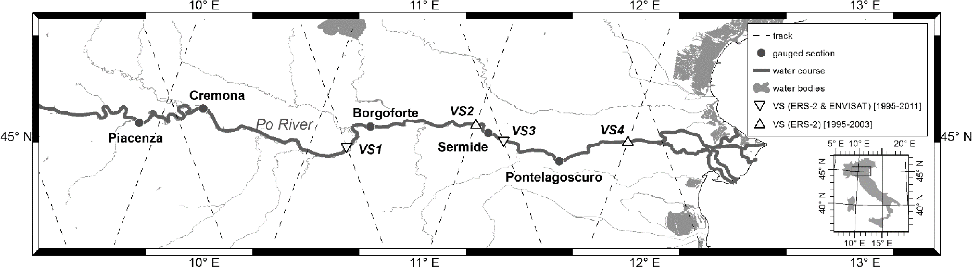
In order to test the proposed methodology for river discharge estimation by satellite altimetry data, the Po River in northern Italy is selected as a case study. It is located in the center of a large flat alluvial plain, the Pianura Padana (Po Valley), and this avoids some issue tied to the presence of mountains that may affect the altimeter echoes. For this study, five gauged river stations along the river, continuously monitoring the water level, are used: Piacenza (basin area equal to 42,030 km2), Cremona (50,726 km2), Borgoforte (62,450 km2), Sermide (68,724 km2) and Pontelagoscuro (70,091 km2) (Figure 1). The geometric characteristics of the five analyzed river stations are deduced by a ground survey carried out by the Interregional Agency of the Po River in 2005 and shown in Table 1. The riverbed consists of a stable main channel with a width varying from 200 to 300 m and two lateral banks (the overall width varies from 400 to 4 km) confined by two artificial levees. The bankfull river depth ranges from about 10 to 18 m. The 236 km river reach bounded by the hydrometric stations of Piacenza and Pontelagoscuro is characterized by the low slope of the river bed bottom and by a significant intermediate drainage area equal to about 40% of the basin, subtended by the downstream station.
The stage and discharge recorded in situ have been provided by the Interregional Agency of the Po River. In particular, daily data of water level, h, for all the stations are selected from May 1995, to August 2010. It must be noted that the knowledge of river discharge, Q, at the selected gauged stations is derived by rating curves obtained by local recorded water levels and velocity measurements, v, occasionally collected for different flow conditions. For each gauged site, at least 25 pairs of h-v values are available, thus allowing one to obtain a reliable stage-discharge relationship. We denote, henceforth, the discharge derived through the rating curve as “observed discharge”.
As regards the flow regime, the values of maximum, mean and minimum discharge of the period 1995–2010 are reported in Table 1 for each gauged site.
4. Radar Altimeter Dataset
At present, various databases are available, enabling the retrieval of water level altimetry time series for large basins, such as Hydroweb [37], the Global Reservoir and Lake Elevation Database [38] and the retracked T/P database within the Contribution of Satellite Altimetry to Hydrology (CASH) project [39]. The altimetry data used in this study came from the database of the processing of ERS-2 and ENVISAT at de Montfort University, UK, on behalf of European Space Agency, ESA [12]. Two types of products are available: (1) the River-Lake Hydrology (RLH) product, intended for hydrologists with no special knowledge of radar altimetry, grouped by the river/lake crossing point (one product per crossing point); (2) the river-lake altimetry (RLA) product, designed for radar-altimetry experts, grouped by satellite orbital revolution. In this work, RLH products are used. The location of the available altimetry data on the Po River is provided in Figure 1 for both ERS-2 (1995–2003) and ENVISAT (2002–2011). The overlap between ERS-2 and ENVISAT allows the data to be adjusted to a common track. Therefore, in total, there are four VSs: four for ERS-2 and two for ENVISAT (overlapping ERS-2 VS1 and VS3) (see Table 2). At each VS, the water level is retrieved every 35 days, but the crossing day differs for each location.
5. Results and Discussion
In this section, first, the comparison between satellite and in situ water level measurements is analyzed, identifying the correlation and the discrepancies among them. Second, the river discharge is estimated through the use of the RCM and BJ03 approaches.
5.1. Comparison between ERS-2 and ENVISAT Data with in Situ Water Level Data
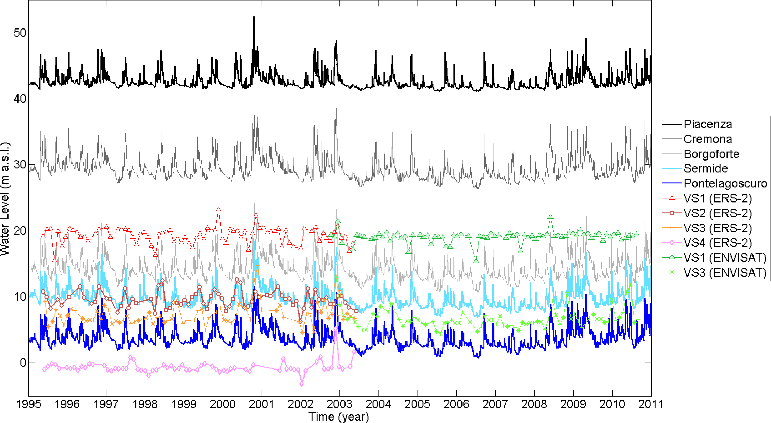
As the first step, both the water level measurements from gauged stations and satellite sensors are referred to the same ellipsoid in order to allow data comparison. As expected, the VSs do not correspond with the gauged stations (see Figure 1 and Table 2). For example, Piacenza and Cremona stations are distant from the nearest VS, 124 km and 77 km, respectively. On the other hand, Sermide station is located between VS2 and VS3, and it is quite near to them (less than 11 km). Figure 2 shows the daily water level time series derived by in situ stations and the 35-day water level time series derived by the radar altimetry. As can be seen, the altimetry data are consistent with in situ measurements, being lower (higher) than the water level recorded at the upstream (downstream) gauged stations. It is worth noting that the ERS-2 data belonging to the VS2 agree very well with the Sermide gauged station, because the mean slope of the river bed between the two sections is very low (0.02%).
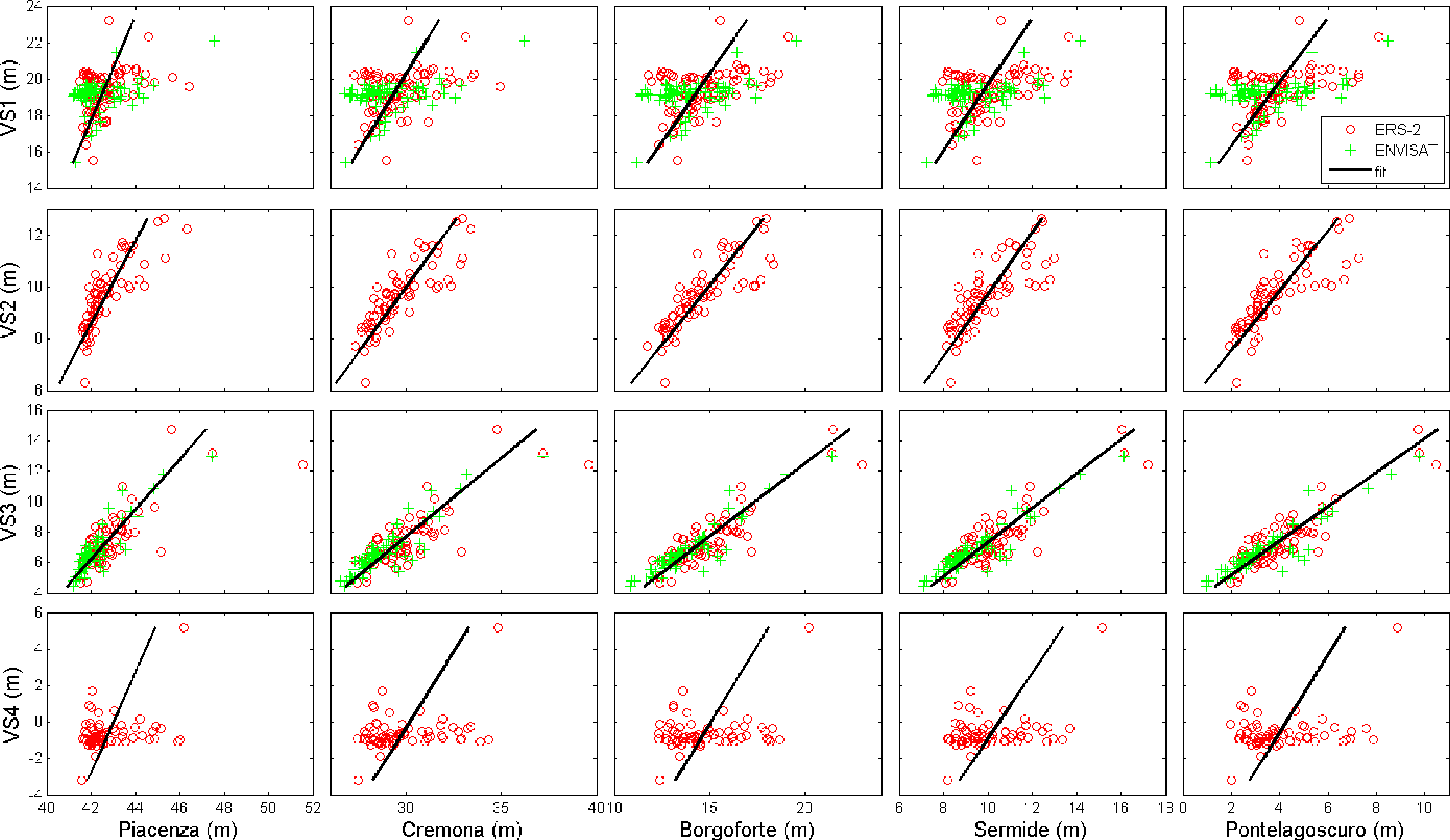
The correlations between the water levels recorded in all the gauged stations and provided at the VSs from altimetry data are reported in Table 3. In particular, the water levels measured in situ are selected during the acquisition dates of the satellite sensor overpasses plus (or minus) the wave travel time, TL, calculated as in Equations (2) and (3), if the VS is upstream (downstream) of the gauged station. The lowest correlation values are obtained when VS4 is considered, and this has to be ascribed to the effect of the mouth of the Po River (see Figure 2). As can be seen in Figure 3, where a scatter plot of the water levels derived from each in situ gauged station and each virtual station is depicted, overall, VS2 and VS3 show a good linear relation with in situ observations (R = 0.79–0.92, Table 1), with the exception of a few data points. Therefore, only these two VSs are selected in the following analyses. Indeed, as regards the VS1, the correlations are quite low for all the gauged stations, ranging from 0.35 to 0.44. For VS1, the actual causes for the obtained inaccuracy are not known and will be the object of future investigations.
In order to evaluate the quantitative accuracy of the satellite data, the water levels derived by satellite altimetry are simulated by using linear regression between satellite observations and in situ measurements; these latter are considered a benchmark (see Table 4). The RMSE values obtained with the VS3 (ERS-2 and ENVISAT series) are similar to the ones obtained with the VS2 (ERS-2 series), but if considered separately, ERS-2 provides higher errors, equal to 0.87 m and 0.85 m for Sermide and Pontelagoscuro, respectively. If ENVISAT data are used, lower RMSE values are obtained for both gauged stations, confirming the statement of Frappart et al. [16], who also found that ENVISAT is more accurate than ERS-2. This is ascribed to a combination of factors. The first factor is the surrounding topography. ENVISAT has the ability to dynamically switch modes when it determines that it is struggling to maintain lock (capture the entire waveform). This means that when the surrounding terrain becomes rough, it can switch from 320 MHz to 80 MHz, and even down to 20 MHz, whilst still retaining information (providing a range window of 64 m, 256 m and 1,024 m, respectively, compared to ERS-2’s 128 m). Therefore, when the terrain becomes less variable, ENVISAT is able to move back up the modes and obtain more waveforms than possible if the lock were lost (such as with ERS-2 and its mask based approach) in the best resolution possible. The second factor is the bin representation. The number of bins for ENVISAT is twice ERS-2 (128 compared to 64). Moreover, the bin width for the ERS-2 altimeter is about 1.82 m wide, whereas for 320 MHz ENVISAT, it is about 47 cm. Therefore, even with retracking when results are obtained from ENVISAT at 320 MHz, they are likely to be more accurate than those from ERS-2.
The estimated accuracy is consistent with previous studies, as, for example, by Birkinshaw et al. [24], who found errors in the term of RMSE in the range 0.46–0.76 m for ERS-2 and 0.44–0.65 m for ENVISAT. The RMSE values obtained for the Po River are slightly higher, but this is expected, as the river channel is much narrower than the Mekong.
The same conclusions can be drawn by examining the NS coefficient values that are found higher for ENVISAT (0.85 for both the stations) than for ERS-2 (0.73 and 0.78 for Sermide and Pontelagoscuro, respectively) for the VS3. Moreover, the NS coefficients for VS3 (ERS-2 and ENVISAT) are much higher than the ones for VS2, despite RMSE being the same. This is ascribed to the variance of the altimetry series belonging to VS2 that is equal to 0.98 m and 1.04 m for Sermide and Pontelagoscuro, respectively, whereas for the VS3, it is found to be almost twice (in the range 1.99–2.39 m).
5.2. Discharge Estimation for Ungauged Sites
The accuracy of RCM to estimate discharge by using satellite data is carried out by comparison with the observed discharge at the closest gauged stations. To this end, we analyze two river reaches: Piacenza-VS2 and Piacenza-VS3. The gauged stations of Sermide and Pontelagoscuro are used as benchmarks, assuming that the contribution of the intermediate drainage area is negligible (see Table 1).
The hydraulic quantities involved in Equation (4), i.e., the water surface width, the average depth and the slope, are applied to the VS2 and VS3, thereby providing a fair comparison of the two approaches.
5.2.1. RCM Application: Piacenza-VS2 River Reach
The analysis is performed by assuming the section geometry available at both river reach ends, while the in situ discharge and the stage are known at the upstream site (Piacenza). The downstream water level data, VS2, are provided by the ERS-2 altimeter in the period 1999–2003 (number of altimetry measurements = 72). Assuming that the downstream station is ungauged, i.e., no flow measurement is available, the parameters of RCM, α and β, are assumed equal to one and zero, respectively. TL is assessed considering the mean flood event (∼3,500 m3·s−1) observed in the upstream station in the entire period by using Equations (2) and (3). The TL value is found equal to 26 h. The results are displayed in Figure 4, and the performance measures are reported in Table 5. The pairs (Qobs, QRCM) overlap the bisector line for both the gauged stations, demonstrating the good agreement of the discharge derived by RCM with in situ observations, even if a slight underestimation is observed, as demonstrated by negative RE (−2.7% and −12.1% for Sermide and Pontelagoscuro, respectively), shown in Table 5. RRMSE is equal to 29% and 27% for Sermide and Pontelagoscuro stations, respectively, and NS is 0.73 for both stations.
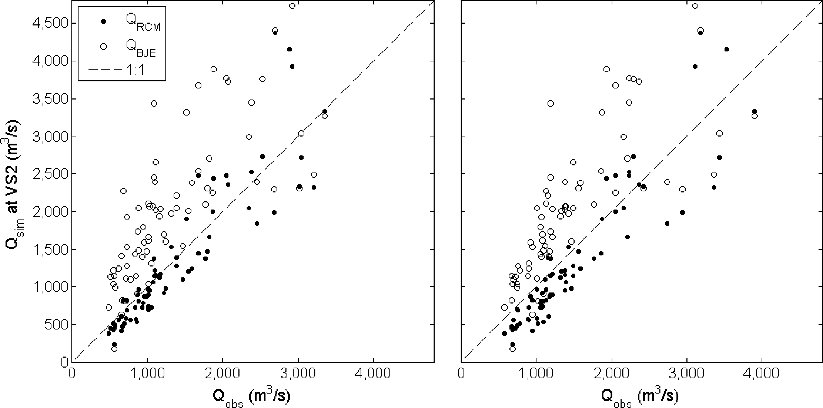
5.2.2. RCM Application: Piacenza-VS3 River Reach
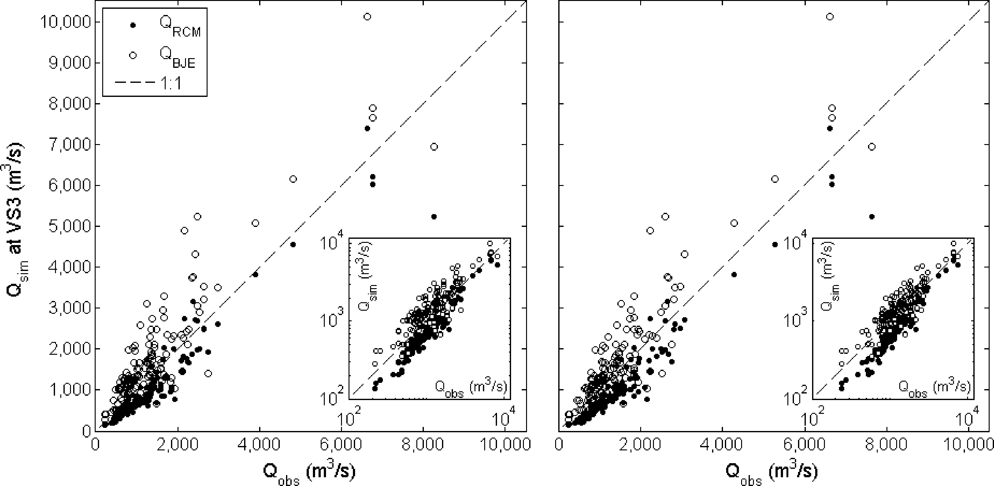
A further analysis is carried out by considering the river reach, Piacenza-VS3. The conditions are the same as the previous case, but the TL is 28 h for a reach of 207 km. The results are shown in Figure 5 for the case in which all the available satellite data are considered, i.e., ERS-2 and ENVISAT. Furthermore, in this case, RCM provides, on average, underestimated discharges, and the pairs (Qobs, QRCM) are below the bisector. RMSE is higher than the one estimated for VS2 (equal to 453 m3·s−1 and 497 m3·s−1), but NS increases up to 0.85 and 0.82, for Sermide and Pontelagoscuro station, respectively (see Table 5). The discharge underestimation in the VS3 is more evident, as confirmed also by RE, which assumes higher values equal to about −20.2% and −25.8% for Sermide and Pontelagoscuro, respectively. If we consider the ERS-2 and ENVISAT time series separately, the results are slightly different. Generally, the RCM approach performs better when the satellite series from ENVISAT are used, as shown by the RMSE being higher for ERS-2 than ENVISAT for both of the gauged stations.
If we compare the observed and simulated discharge considering only ERS-2 altimetry data, RCM works better for VS2 (ERS-2) with RMSE, RRMSE and RE errors lower than the ones computed for VS3 (ERS-2).
The use of constant and uncalibrated values for the parameters, α and β, produces both the underestimation of RCM discharge and the scattering of the pairs (Qobs, QRCM) in Figure 5. Indeed, the underestimation may be also ascribed to the overestimation of the upstream effective flow area (Piacenza section) where the water levels affect the floodplains and the flow area is likely overestimated [40]. Moreover, the scattering also depends on the flow area at the VS that is computed through a single cross-section survey available in the area of the satellite track. Therefore, the possible changes in the cross-section geometry are not taken into account.
Generally, RCM provides satisfactory results, confirming the potential usefulness of the method to be used with satellite data for the estimation of the discharge. Moreover, these errors are consistent with the ones of the study carried out by Getirana et al. [22], who obtained RE ranging from 8.4% to 19.7% by using a rainfall-runoff model for the discharge estimation in the Branco River in the Amazon basin.
5.2.3. Application of Empirical Equation Derived by Bjerklie et al. [27]
For the application of the empirical equation, BJ03, the slope, S, is calculated considering the average value of the altimetry levels at both sections, VS2 and VS3, and the distance between them (17 km), and it is equal to 0.00014. For the other two quantities, W and Y, the values are based on the section survey that is assumed to be known. In particular, the top width, W, is estimated considering the level of bankfull, equal to 400 and 377 m for VS2 and VS3, respectively. For the calculation of depth, Y, we subtract from the water level elevation derived from radar altimetry the elevation of the cross-section bottom, z0. The latter is computed referring to the equivalent rectangular section at the bankfull level, and hence, it is estimated considering the bankfull cross-section area divided by the corresponding width of the section, W.
In Figures 4 and 5, the discharges obtained through the use of BJ03 are shown and compared with the observations. As can be seen in Table 5, differently from RCM, the application of BJ03 for VS2 does not provide satisfactory results. RMSE (962 m3·s−1 and 834 m3·s−1 for Sermide and Pontelagoscuro, respectively) and the RRMSE values (70.5% and 55.3%) are quite high, whereas negative NS values are obtained. This result is due to an important overestimation of BJ03, clearly visible in Figure 4.
Furthermore, by considering the VS3 (ERS-2 and ENVISAT), errors are found to be higher than the ones referring to RCM, above all for the Sermide section, with RMSE, RRMSE and NS equal to 755 m3·s−1, 54.3% and 0.59, respectively. For Pontelagoscuro section, the performance measures are slightly better, with RMSE, RRMSE and NS values of 670 m3·s−1, 45% and 0.66, respectively. Additionally, in this case, altimetry data from ENVISAT are better than ERS-2 ones, as shown in Table 5. Moreover, the discharges estimated by BJ03 are overestimated, as confirmed by RE that is positive for both the VSs ranging from 20% for VS3 (ENVISAT) at Pontelagoscuro to 53% at VS2 (ERS-2). Better results were obtained by Birkinshaw et al. [25], applying the same empirical equation in the Mekong and Ob rivers, with NS values ranging between 0.86 and 0.90. However, the strong seasonality of the rivers investigated by Birkinshaw et al. [25] surely enhance the obtained NS values [41]. Moreover, in Birkinshaw et al. [25] measurements were taken along a 50 km reach of river to account for short-scale variability of natural river morphology, rather than at a specific location. This aspect might be another reason for the lower NS values here obtained.
It is worth noting that RCM takes into account the discharge recorded at the upstream section, whereas BJ03 does not consider this input data. Furthermore, also, the application of the BJ03 in Italy should be preceded by a calibration of the coefficients by using the in situ measurements.
6. Conclusions
In this study, river discharge is estimated for two gauged sites on the Po River by using altimetry data from ERS-2 and ENVISAT satellites. The comparison between the satellite and in situ water level measurements has shown that the accuracy of the altimetry data depends on the satellite sensor. ERS-2 is found to be less accurate than ENVISAT, as shown at the VS3, where comparison with the observed water levels provides errors of about 60 cm and 81 cm for ENVISAT and ERS-2, respectively (see Table 4). An issue to address is how to filter out inaccurate radar altimetry data (e.g., at VS1) without considering the ground data.
The study uses two methods for the discharge estimation in the ungauged river site, where only the geometry of the cross-sections is required. The proposed simplified routing model, named RCM, applied with altimetry data, is able to estimate the discharge in a river site narrower than the one usually considered for altimetry applications [25]. Despite that a slight underestimation can be observed in both gauged stations (see Figures 4 and 5), Sermide and Pontelagoscuro, a low RRMSE nearly equal to 30% is obtained (see Table 5).
Moreover, the RCM method outperformed the empirical formula proposed by Bjerklie et al. [27], which, however, does not use the knowledge of discharge at an upstream river section. If the data of velocity and water level for different flow conditions would have been available for the investigated river reaches, it is expected that Bjerklie’s equation would have provided better performance by an appropriate calibration of parameters.
The obtained results suggest that the radar altimetry observations can be used to estimate discharge at ungauged river sites. An open issue that has still to be addressed is related to the assessment of the cross-section geometry [42] and, specifically, the estimation of the elevation of the cross-section bottom [43].
Future investigations will be performed to integrate altimetry-derived water levels and velocity data derived by Moderate Resolution Imaging Spectroradiometer, MODIS [44] for further improvement of discharge estimation in ungauged river sites.
Acknowledgments
The authors wish to thank the European Space Agency for furnishing the altimetry data, ARPA (Agenzia Regionale Prevenzione e Ambiente) Emilia Romagna and, in particular, Eng. Federica Pellegrini, for providing the analyzed data for the Po River basin.
Conflict of Interest
The authors declare no conflict of interest.
References and Notes
- Chow, V.T.; Maidment, D.; Mays, L. Applied Hydrology; McGraw-Hill: New York, NY, USA, 1988. [Google Scholar]
- Moramarco, T.; Saltalippi, C.; Singh, V.P. Estimating the cross-sectional mean velocity in natural channels using Chiu’s velocity distribution. J. Hydrol. Eng 2004, 9, 42–50. [Google Scholar]
- Di Baldassarre, G.; Montanari, A. Uncertainty in river discharge observations: A quantitative analysis. Hydrol. Earth Syst. Sci 2009, 13, 913–921. [Google Scholar]
- Vorosmarty, C.; Birkett, C.; Dongman, L.; Lettenmaier, D.P.; Kim, Y.; Rodriguez, E.; Emmit, G.D.; Plant, W.; Wood, E. NASA Post-2002 Land Surface Hydrology Mission Component for Surface Water Monitoring, HYDRA_SAT HYDRlogical Altimetry SATellite. Proceedings of NASA Post 2002 LSHP Planning Workshop, Irvine, CA, USA, 12–14 April 1999; p. 53.
- Calmant, S.; Seyler, F. Continental surface water from satellite altimetry. Compt. Rend. Geosci 2006, 338, 1113–1122. [Google Scholar]
- IAHS Ad Hoc Committee. Global water data: A newly endangered species. EOS Trans. AGU 2001, 82, 54.
- Biancamaria, S.; Hossain, F.; Lettenmaier, D.P. Forecasting transboundary river water elevations from space. Geophys. Res. Lett 2011, 38, L11401. [Google Scholar]
- Birkett, C.M. The contribution of Topex/Poseidon to the global monitoring of climatically sensitive lakes. J. Geophys. Res 1995, 100, 25179–25204. [Google Scholar]
- Coe, M.T.; Birkett, C.M. Calculation of river discharge and prediction of lake height from satellite radar altimetry: example for the Lake Chad basin. Water Resour. Res 2004, 40, W10205. [Google Scholar]
- Morris, C.S.; Gill, S.K. Variation of Great-Lakes water levels derived from Geosat altimetry. Water Resour. Res 1994, 30, 1009–1017. [Google Scholar]
- Calman, S.; Seyler, F.; Cretaux, J.F. Monitoring continental surface waters by satellite altimetry. Surv. Geophys 2008, 29, 247–269. [Google Scholar]
- Global NRT Product Locations. Available online: http://earth.esa.int/riverandlake (accessed on 30 May 2013).
- Koblinsky, C.J.; Clarke, R.T.; Brenner, A.C.; Frey, H. Measurement of River Level variations with Satellite Altimetry. Water Resour. Res 1993, 29, 1839–1848. [Google Scholar]
- Birkett, C.M. Contribution of the Topex NASA radar altimeter to the global monitoring of large rivers and wetlands. Water Resour. Res 2004, 34, 1223–1239. [Google Scholar]
- De Oliveira Campos, I.; Mercier, F.; Maheu, C.; Cochonneau, G.; Kosuth, P.; Blitzkow, D.; Cazenave, A. Temporal variations of river basin waters from Topex/ Poseidon satellite altimetry. Application to the Amazon basin. Comp. Rend. l’Acad. Sci.–Series IIA–Earth Planet. Sci 2001, 333, 633–643. [Google Scholar]
- Frappart, F.; Calmant, S.; Cauhope, M.; Seyler, F.; Cazenave, A. Preliminary results of ENVISAT RA-2-derived water levels validation over the Amazon basin. Remote Sens. Environ 2006, 100, 252–264. [Google Scholar]
- Leon, J.G.; Calmant, S.; Seyler, F.; Bonnet, M.P.; Cauhope, M.; Frappart, F.; Filizola, N.; Fraizy, P. Rating curves and estimation of average water depth at the upper Negro River based on satellite altimeter data and modeled discharges. J. Hydrol 2006, 328, 481–496. [Google Scholar]
- Zakharova, E.A.; Kouraev, A.V.; Cazenave, A.; Seyler, F. Amazon River discharge estimated from TOPEX/Poseidon altimetry. Compt. Rend. Geosci 2006, 338, 188–196. [Google Scholar]
- Santos da Silva, J.; Calmant, S.; Seyler, F.; Rotunno Filho, O.C.; Cochonneau, G.; Mansur, W.J. Water levels in the Amazon basin derived from the ERS 2 and ENVISAT radar altimetry missions. Remote Sens. Environ 2010, 114, 2160–2181. [Google Scholar]
- Kouraev, A.V.; Zakharova, E.A.; Samain, O.; Mognard, N.M.; Cazenave, A. Ob’ river discharge from TOPEX/Poseidon satellite altimetry (1992–2002). Remote Sens. Environ 2004, 93, 238–245. [Google Scholar]
- Frappart, F.; Seyler, F.; Martinez, J.M.; Leon, J.G.; Cazenave, A. Floodplain water storage in the Negro River basin estimated from microwave remote sensing of inundation area and water levels. Remote Sens. Environ 2005, 99, 387–399. [Google Scholar]
- Getirana, A.C.V.; Bonnet, M.P.; Calmant, S.; Roux, E.; Rotunno, O.C.; Mansur, W.J. Hydrological monitoring of poorly gauged basins based on rainfall-runoff modeling and spatial altimetry. J. Hydrol 2009, 379, 205–219. [Google Scholar]
- Pereira-Cardenal, S.J.; Riegels, N.D.; Berry, P.A.M.; Smith, R.G.; Yakovlev, A.; Siegfried, T.U.; Bauer-Gottwein, P. Real-time remote sensing driven river basin modeling using radar altimetry. Hydrol. Earth Syst. Sci 2009, 15, 241–254. [Google Scholar]
- Birkinshaw, S.J.; O’Donnell, G.M.; Moore, P.; Kilsby, C.G.; Fowler, H.J.; Berry, P.A.M. Using satellite altimetry data to augment flow estimation techniques on the Mekong River. Hydrol. Process 2010, 24, 3811–3825. [Google Scholar]
- Birkinshaw, S.J.; Moore, P.; Kilsby, C.G.; O’Donnell, G.M.; Hardy, A.J.; Berry, P.A.M. Daily discharge estimation at ungauged river sites using remote sensing. Hydrol. Process. 2012. [Google Scholar] [CrossRef]
- Birkett, C.M.; Mertes, L.; Dunne, T.; Costa, M.H.; Jasinski, M.J. Surface water dynamics in the Amazon Basin: Application of satellite radar altimetry. J. Geophys. Res. 2002, 107. [Google Scholar] [CrossRef]
- Bjerklie, D.M.; Dingman, S.L.; Vorosmarty, C.J.; Bolster, C.H.; Congalton, R.G. Evaluating the potential for measuring river discharge from space. J. Hydrol 2003, 278, 17–38. [Google Scholar]
- Getirana, A.C.V. Integrating spatial altimetry data into the automatic calibration of hydrological models. J. Hydrol 2010, 387, 244–255. [Google Scholar]
- Milzow, C.; Krogh, P.E.; Bauer-Gottwein, P. Combining satellite radar altimetry, SAR surface soil moisture and GRACE total storage changes for hydrological model calibration in a large poorly gauged catchment. Hydrol. Earth Syst. Sci 2010, 15, 1729–1743. [Google Scholar]
- Sun, W.C.; Ishidaira, H.; Bastola, S. Towards improving river discharge estimation in ungauged basins: Calibration of rainfall-runoff models based on satellite observations of river flow width at basin outlet. Hydrol. Earth Syst. Sci 2010, 14, 2011–2022. [Google Scholar]
- Moramarco, T.; Singh, V.P. Simple method for relating local stage and remote discharge. J. Hydrol. Eng 2001, 6, 78–81. [Google Scholar]
- Moramarco, T.; Barbetta, S.; Melone, F.; Singh, V.P. Relating local stage and remote discharge with significant lateral inflow. J. Hydrol. Eng 2005, 10, 58–69. [Google Scholar]
- Barbetta, S.; Franchini, M.; Melone, F.; Moramarco, T. Enhancement and comprehensive evaluation of the Rating Curve Model for different river sites. J. Hydrol. 2012, 464–465, 376–387. [Google Scholar]
- Nash, J.E.; Sutcliffe, J.V. River flow forecasting through conceptual models, Part I: A discussion of principles. J. Hydrol 1970, 10, 282–290. [Google Scholar]
- Barbetta, S.; Moramarco, T.; Franchini, M.; Melone, F.; Brocca, L.; Singh, V.P. Case study: Improving real-time stage forecasting Muskingum model by incorporating the Rating Curve Model. J. Hydrol. Eng 2011, 16, 540–557. [Google Scholar]
- Tayfur, G.; Barbetta, S.; Moramarco, T. Genetic Algorithm based discharges estimation at sites receiving lateral inflows. J. Hydrol. Eng 2009, 14, 463–474. [Google Scholar]
- Lakes, Rivers and Wetlands Water Levels from Satellite Altimetry. Available online: http://www.legos.obs-mip.fr/en/soa/hydrologie/hydroweb/ (accessed on 30 May 2013).
- Crop Explorer. Available online: http://www.pecad.fas.usda.gov/cropexplorer/global_reservoir/ (accessed on 30 May 2013).
- CASH, Contribution of Satellite Altimetry to Hydrology. Available online: http://www.cls.fr/html/oceano/general/applications/cash_en.html (accessed on 15 July 2013).
- Barbetta, S.; Brocca, L.; Tarpanelli, A.; Melone, F.; Singh, V.P.; Moramarco, T. Discharge Assessment at Ungauged River Sites by Using Satellite Altimetry Data: The Case Study of the Po River (Italy). Proceedings of International Conference 6th International Perspective on Water Resources & the Environment Conference (IPWE 2013), Izmir, Turkey, 7–9 January 2013; p. 10.
- Khan, S.I.; Hong, Y.; Vergara, H.J.; Gourley, J.J.; Brakenridge, G.R.; De Groeve, T.; Flaming, Z.L.; Policelli, F.; Yong, B. Microwave Satellite data for hydrologic modeling in ungauged basins. IEEE Geosci. Remote Sens. Lett 2012, 9, 663–667. [Google Scholar]
- Moramarco, T.; Corato, G.; Melone, F.; Singh, V.P. An entropy-based method for determining the flow depth distribution in natural channels. J. Hydrol 2013, 497, 176–188. [Google Scholar]
- Mersel, M.K.; Smith, L.C.; Andreadis, K.M.; Durand, M.T. Estimation of river depth from remotely sensed hydraulic relationships. Water Resour. Res 2013, 49, 1–15. [Google Scholar]
- Tarpanelli, A.; Brocca, L.; Melone, F.; Moramarco, T.; Lacava, T.; Faruolo, M.; Pergola, N.; Tramutoli, V. Toward the estimation of river discharge variations using MODIS data in ungauged basins. Remote Sens. Environ 2013, 136, 47–55. [Google Scholar]


| Gauged Station | Ab (km2) | w (m) | D (m) | Qmax (m3·s−1) | Qmin (m3·s−1) | Qm (m3·s−1) |
|---|---|---|---|---|---|---|
| Piacenza | 42,030 | 213 | 18.01 | 12,800 | 125 | 958 |
| Cremona | 50,726 | 278 | 12.86 | 13,750 | 200 | 1,115 |
| Borgoforte | 62,450 | 266 | 10.47 | 12,047 | 209 | 1,373 |
| Sermide | 68,724 | 493 | 11.19 | 10,100 | 123 | 1,358 |
| Pontelagoscuro | 70,091 | 302 | 18.73 | 10,300 | 156 | 1,501 |
| Virtual Stations | Gauged Stations | ||||
|---|---|---|---|---|---|
| Piacenza | Cremona | Borgoforte | Sermide | Pontelagoscuro | |
| VS1 | 124 | 77 | −20 | −77 | −112 |
| VS2 | 190 | 144 | 47 | −11 | −46 |
| VS3 | 207 | 160 | 63 | 6 | −29 |
| VS4 | 264 | 217 | 120 | 63 | 28 |
| Satellite | Data Availability | Gauged Stations | ||||
|---|---|---|---|---|---|---|
| Piacenza | Cremona | Borgoforte | Sermide | Pontelagoscuro | ||
| VS1 (ERS-2 and ENVISAT) | 1995–2010 | 0.37 | 0.38 | 0.42 | 0.42 | 0.43 |
| VS1 (ERS-2) | 1995–2003 | 0.35 | 0.37 | 0.43 | 0.42 | 0.44 |
| VS1 (ENVISAT) | 2002–2010 | 0.40 | 0.39 | 0.40 | 0.41 | 0.42 |
| VS2 (ERS-2) | 1995–2003 | 0.79 | 0.83 | 0.83 | 0.79 | 0.82 |
| VS3 (ERS-2 and ENVISAT) | 1995–2010 | 0.81 | 0.85 | 0.90 | 0.89 | 0.91 |
| VS3 (ERS-2) | 1995–2003 | 0.75 | 0.81 | 0.87 | 0.86 | 0.89 |
| VS3 (ENVISAT) | 2002–2010 | 0.89 | 0.90 | 0.92 | 0.92 | 0.92 |
| VS4 (ERS-2) | 1995–2003 | 0.31 | 0.32 | 0.31 | 0.35 | 0.30 |
| Satellite | Number of Altimetry Measurements | Sermide | Pontelagoscuro | ||
|---|---|---|---|---|---|
| RMSE (m) | NS | RMSE (m) | NS | ||
| VS2 (ERS-2) | 72 | 0.80 | 0.63 | 0.75 | 0.67 |
| VS3 (ERS-2 and ENVISAT) | 148 | 0.76 | 0.79 | 0.69 | 0.82 |
| VS3 (ERS-2) | 72 | 0.87 | 0.73 | 0.75 | 0.78 |
| VS3 (ENVISAT) | 76 | 0.59 | 0.85 | 0.61 | 0.85 |
| Satellite | Sermide | |||||||
|---|---|---|---|---|---|---|---|---|
| RCM | BJ03 | |||||||
| RMSE (m3·s−1) | RRMSE (%) | NS (−) | RE (%) | RMSE (m3·s−1) | RRMSE (%) | NS (−) | RE (%) | |
| VS2 (ERS-2) | 396 | 29.0 | 0.73 | −2.7 | 962 | 70.5 | −0.61 | 52.9 |
| VS3 (ERS-2 and ENVISAT) | 453 | 32.6 | 0.85 | −20.2 | 755 | 54.3 | 0.59 | 29.6 |
| VS3 (ERS-2) | 530 | 33.4 | 0.84 | −17.3 | 892 | 56.2 | 0.54 | 29.2 |
| VS3 (ENVISAT) | 365 | 30.3 | 0.87 | −23.9 | 597 | 49.6 | 0.64 | 30.2 |
| Satellite | Pontelagoscuro | |||||||
|---|---|---|---|---|---|---|---|---|
| RCM | BJ03 | |||||||
| RMSE (m3·s−1) | RRMSE (%) | NS (−) | RE (%) | RMSE (m3·s−1) | RRMSE (%) | NS (−) | RE (%) | |
| VS2 (ERS-2) | 405 | 26.9 | 0.73 | −12.1 | 834 | 55.3 | −0.14 | 38.3 |
| VS3 (ERS-2 and ENVISAT) | 497 | 33.3 | 0.82 | −25.8 | 670 | 44.9 | 0.66 | 20.6 |
| VS3 (ERS-2) | 526 | 31.2 | 0.82 | −22.3 | 794 | 47.0 | 0.60 | 21.3 |
| VS3 (ENVISAT) | 467 | 35.7 | 0.80 | −30.1 | 527 | 40.3 | 0.74 | 19.8 |
© 2013 by the authors; licensee MDPI, Basel, Switzerland This article is an open access article distributed under the terms and conditions of the Creative Commons Attribution license ( http://creativecommons.org/licenses/by/3.0/).
Share and Cite
Tarpanelli, A.; Barbetta, S.; Brocca, L.; Moramarco, T. River Discharge Estimation by Using Altimetry Data and Simplified Flood Routing Modeling. Remote Sens. 2013, 5, 4145-4162. https://doi.org/10.3390/rs5094145
Tarpanelli A, Barbetta S, Brocca L, Moramarco T. River Discharge Estimation by Using Altimetry Data and Simplified Flood Routing Modeling. Remote Sensing. 2013; 5(9):4145-4162. https://doi.org/10.3390/rs5094145
Chicago/Turabian StyleTarpanelli, Angelica, Silvia Barbetta, Luca Brocca, and Tommaso Moramarco. 2013. "River Discharge Estimation by Using Altimetry Data and Simplified Flood Routing Modeling" Remote Sensing 5, no. 9: 4145-4162. https://doi.org/10.3390/rs5094145