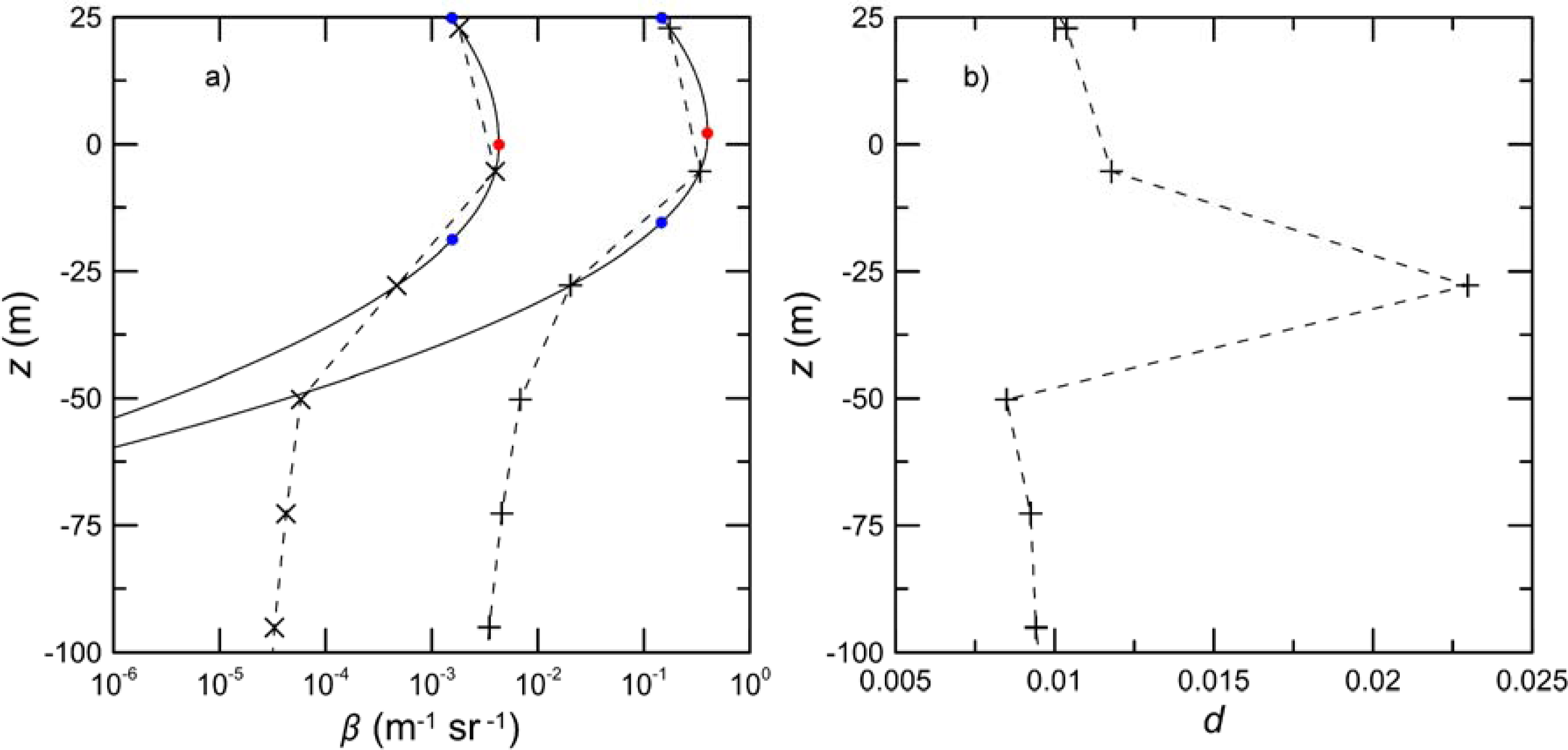
Article

Subsurface Ocean Signals from an Orbiting Polarization Lidar

1
Earth System Research Laboratory, National Oceanic and Atmospheric Administration, 325 Broadway, Boulder, CO 80305, USA
2
Cooperative Institute for Research in Environmental Sciences, University of Colorado, 325 Broadway, Boulder, CO 80305, USA
3
Langley Research Center, National Aeronautics and Space Administration, Hampton, VA 23666, USA
*
Author to whom correspondence should be addressed.
Remote Sens. 2013, 5(7), 3457-3475; https://doi.org/10.3390/rs5073457
Submission received: 28 May 2013 / Revised: 15 July 2013 / Accepted: 17 July 2013 / Published: 19 July 2013
(This article belongs to the Special Issue Remote Sensing of Phytoplankton)

Abstract

:
Detection of subsurface returns from the Cloud-Aerosol Lidar with Orthogonal Polarization (CALIOP) on the Cloud-Aerosol Lidar and Infrared Pathfinder Satellite Observation (CALIPSO) satellite were demonstrated. Despite the coarse range resolution of this aerosol lidar, evidence of subsurface scattering was observed as a delay and broadening of the cross-polarized signal relative to the co-polarized signal in the three near-surface range bins. These two effects contributed to an increased depolarization at the nominal depth of 25 m. These features were all correlated with near-surface chlorophyll concentrations. An increase in the depolarization was also seen at a depth of 50 m under certain conditions, suggesting that chlorophyll concentration at that depth could be estimated if an appropriate retrieval technique can be developed. At greater depths, the signal is dominated by the temporal response of the detectors, which was approximated by an analytical expression. The depolarization caused by aerosols in the atmosphere was calculated and eliminated as a possible artifact.

1. Introduction

Airborne lidar operating at a wavelength of 532 nm has proven to be an effective tool for probing the upper ocean. Studies include detection of fish and zooplankton [15], thin plankton layers [6], internal waves propagating on the pycnocline [7,8], and bubbles [9,10]. Extending these capabilities to a satellite-based lidar would provide the depth dimension that is missing in satellite-based ocean-color measurements.
The Cloud-Aerosol Lidar with Orthogonal Polarization (CALIOP) is the primary instrument on the Cloud-Aerosol Lidar and Infrared Pathfinder Satellite Observation (CALIPSO) satellite. This lidar has many of the same characteristics as the airborne lidars, including the 532 nm laser wavelength, a laser pulse length of 10–20 ns, and dual-polarization receivers [11]. These characteristics suggest that the CALIOP might be useful for oceanographic studies, even though its mission is to investigate clouds and aerosols in the atmosphere. Our objective in this paper was to determine whether or not there was a subsurface component to the CALIOP return over the ocean.
There have been several investigations of CALIOP subsurface signals. Rodier et al. [12] estimated the subsurface lidar signal from the depth-integrated, cross-polarized lidar signal, and compared that with surface chlorophyll concentration on a global scale. Shi and Wang [13] compared the total signal in the nominal surface bin (reported altitude of −7 m) and the first subsurface bin (nominal altitude −37 m) in the Gulf of Martaban in the eastern Indian Ocean before and after passage of Cyclone Nargis in 2008. They used the relative values in these two depth bins to argue for vertical mixing of sediments by the cyclone. Barton and Jasinski [14] used the total return integrated over the nominal surface bin and all subsurface bins to estimate total subsurface scattering in Tampa Bay, Florida. This estimate was based on corrections for atmospheric attenuation and for surface reflections, including specular reflections and scattering from surface foam. The surface reflection components were based on models involving the wind speed.
Despite these investigations, there are several difficulties in applying CALIOP data to subsurface scattering. The primary difficulty is the processing of the signals prior to downlink. The data are filtered to condense the signal profiles in range, ultimately decreasing the downlinked data volume. The lidar returns are low-pass filtered with a three-pole Bessel filter with a bandwidth of 2 MHz and digitized at a rate of 10 MHz, corresponding to the initial 15 m range sampling. Two successive samples are averaged to provide a range resolution of 30 m in air or 22.5 m in water. Another factor is that the incidence angle was 0.3° until November of 2007 and 3° after this date. Airborne lidars typically operate with an incidence angle of around 15° to reduce the specular reflection from the surface. The CALIOP has a very strong specular component, and this component has been suggested as a technique to infer wind speed [15]. One other difficulty is a slow transient recovery time of the photomultiplier tubes used in the detection of the 532 nm channels. This detector feature can mask weak subsurface returns [16].
We considered several characteristics of lidar returns that included a subsurface contribution to determine whether the CALIOP could, in fact, respond to subsurface scattering. The specular return from the sea surface preserves polarization, but subsurface scattering depolarizes initially polarized light [1719]. Therefore, we concentrated on a comparison of the CALIOP 532 channels, the cross-polarized return and the total, or unpolarized, return.
The null hypothesis for this study was that there was no contribution to the signal from below the surface of the ocean. This hypothesis implies no depolarization of the return near the surface, since the surface itself is a polarization-preserving specular reflector. It further implies that the shape of the cross-polarized return would be identical to the shape of the unpolarized return, since the only source of depolarization would be incomplete polarization separation in the lidar. Finally, the null hypothesis implies that there would be no correlation between any characteristics of the lidar return and subsurface properties like phytoplankton concentration. Conversely, the null hypothesis would be refuted if there is a significant depolarization at ranges corresponding to below the surface, since this could only come from subsurface scatterers. Alternatively, it would be refuted if the broad surface return in the cross-polarized receiver were delayed or further broadened relative to the unpolarized return, since this could only come from scattering occurring after the surface reflection. If the distribution of these properties were correlated with near-surface chlorophyll concentration, used as a proxy for scatterer density, this would provide additional evidence to refute the null hypothesis.
We restricted the analysis to regions of relatively clear, open-ocean waters. In very turbid water, the lidar signal attenuates rapidly. The near-surface return would be partially depolarized by subsurface return, but the cross-polarized pulse delay and broadening would be very small. In addition, the delay and broadening would be affected more by penetration depth than the concentration of subsurface scatterers, so one might expect a negative correlation with chlorophyll concentration for these cases.

2. Materials and Methods

The primary data set comprised the version 3.01, level 1b CALIOP total attenuated backscatter, βT, and cross-polarized attenuated backscatter, βX, for the year 2010 and for latitudes between 60°S and 60°N [20]. Only the 532 nm wavelength was used, because the 1064 nm light is strongly absorbed by sea water. Daytime data were removed to minimize noise from background light. To avoid turbid coastal waters, the associated land/water mask was used to exclude all but deep-ocean data (>120 m). The level 2 cloud layer product was used to remove profiles contaminated by clouds. Similarly, the aerosol optical depths, AOD as available in the level 2 aerosol layer product and estimated from the CALIOP profiles, were used to remove profiles with AOD > 0.2 minimizing possible contamination by aerosols. Lidar shots were also removed from the data set if maximum signals were so small (βT < 0.1 m−1·sr−1 or βX < 0.001 m−1·sr−1) that the resulting profiles were very noisy.
The lidar calibration is described in detail [11], but is briefly reviewed here. The 532 nm total return was calibrated using backscatter from altitudes between 30 and 34 km above mean sea level, where the atmosphere is purely molecular and the expected return can be accurately estimated. The calibration coefficient was measured during the nighttime segment of each orbit and averaged over 1485 km of ground track. The 532 nm cross-polarized channel calibration coefficient was calculated from that of the total channel using a factor that was periodically measured by inserting a pseudo-depolarizer into the optical path before the polarization beam splitter.
The CALIOP data are reported at a vertical resolution of 30 m in the altitude region between −0.5 and 8.3 km above the surface, but the exact altitude changes with variations in satellite orbit. A shift of several range bins may be necessary to account for these differences. It is because of this uncertainty in altitude that data are reported to 0.5 km below the surface. Not because useful data were expected at this depth, but to ensure that the atmosphere was sampled to the surface. A suggested shift in altitude bins is provided with the level 1b data based on estimated orbital parameters, and we applied this shift to the data. For each polarization channel, an additional shift of one range bin in either direction was applied if the peak of the attenuated backscatter was one bin above or below the nominal surface bin. If the peak was more than one bin from the nominal surface bin in either channel, that shot was not used in the analysis.
For each of the remaining lidar shots and for each channel, the nominal surface sample and the two adjacent samples were selected to calculate the three parameters of a Gaussian curve. These parameters are the amplitude, A, the altitude of the peak, R, and the width, W, so
β ( z ) = A exp [ ( z R ) 2 W 2 ] ,
where z is the altitude in air. The parameters were calculated using values for z of 22.8 m, −7.1 m, and −37.1 m and the corresponding data values for each shot. The nominal surface bin at −7.1 m in air corresponds to a depth of 5.3 m and the first subsurface bin at −37.1 m corresponds to a depth of 27.9 m. We then calculated the differences ΔR = RTRX and ΔW = WXWT. The altitude difference between the two channels was used rather than the absolute altitude in the cross-polarized channel, because the absolute altitude of the surface (as defined in the lidar altitude bins) is not known precisely [16]. Use of the difference removes this uncertainty. Similarly, the width difference removes any effects that would be common to both channels, such as a temporal spreading of the surface return by waves. Note that these differences were defined such that both are positive if the cross-polarized return is delayed and broadened when compared with the total. These differences, ΔR and ΔW, were averaged into one degree latitude and longitude bins by month.
The depolarization was defined as
d ( z ) = β X ( z ) β T ( z ) β X ( z ) ,
and the values in the first subsurface bin (z = −27.9 m) were averaged in the same way as ΔR and ΔW.
A total of 9.6 million lidar shots passed all of the criteria and were used in the analysis. The number in each one degree by one degree by one month average ranged from 0 to 555. Of these, 139,242 contained at least one shot, with an average number of 69.
One other dataset used in the analysis was chlorophyll-a concentration, C, derived from the Moderate Resolution Imaging Spectroradiometer (MODIS) on the Aqua satellite [21]. Chlorophyll concentration was estimated using the three-band OC3 algorithm using a polynomial fit in the logarithm of the ratio of blue to green remote-sensing reflectance. In this algorithm, the blue remote-sensing reflectance is the larger of that at 443 nm or 489 nm, and the green is that at 550 nm. Monthly averaged, level 3 data with 4 km resolution were averaged to the same one degree latitude and longitude bins as the CALIOP data.
An observed correspondence in the spatial patterns of the lidar data and the chlorophyll concentration was investigated quantitatively using Spearman’s rank correlation of the one degree by one degree monthly averages.
Wind speed for each CALIOP profile was obtained from the level 2b data from the Advanced Microwave Scanning Radiometer—Earth Observing System (AMSR-E) sensor on NASA’s Aqua satellite [22]. While the spatial resolution of the AMSR-E wind product is much larger than the CALIOP footprint, the root-mean-square difference between that and the wind speed inferred directly from CALIOP is only 1.2 m·s−1 for clear skies [15], which is sufficient for our purposes.

3. Results and Discussion

A typical profile (Figure 1a) shows the delay and broadening of the cross-polarized return relative to the total return as described in the introduction. This example was averaged over 100 lidar shots to show the general features without noise. The standard deviations of the 100 values at each depth were around 20% of the corresponding means for the total return and almost 100% for the cross-polarized return. Much of this variability is probably a result of surface roughness variations, but a detailed investigation is beyond the scope of this paper. The amplitude, AT, of the Gaussian fit to the total surface return peaks at 2.2 m above the surface, while the amplitude, AX, of the fit to the cross-polarized return peaks at 0.2 m below the surface, so ΔR = 2.4 ± 0.2 m. The width, WT, of the total return is 22.8 m, while the width of the cross-polarized return, WX, is 24.8 m, so ΔW = 2.0 ± 0.4 m. The variability in the single-shot parameter values is also large, but the resulting uncertainties in average ΔR and ΔW for this example are 9% and 18%, respectively. The depolarization of the same averaged profile (Figure 1b) shows a maximum in the depolarization at a depth of 28 m. This is consistent with subsurface scattering. This figure also shows the effects of the relatively slow transient response of the photomultiplier tubes for both channels.
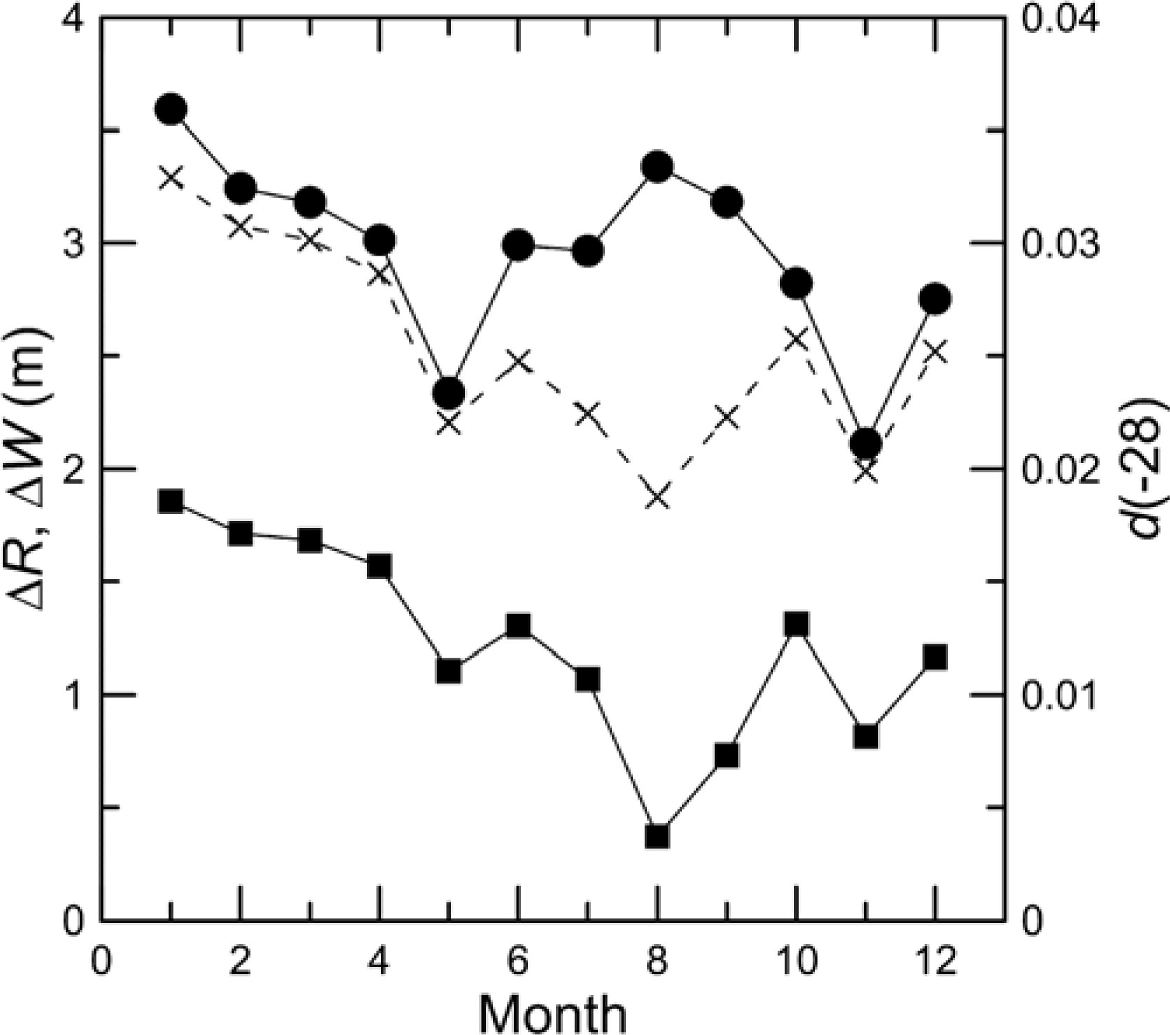
For all months of 2010, the global averages (60°S to 60°N) of both ΔR and ΔW (Figure 2) were significantly greater than zero. The number of lidar shots contributing to those monthly averages ranged from 0.4 million in August to 1.6 million in March. Despite the shot-to-shot variability, the large number of shots in each average resulted in a standard deviation of each average that was less than 0.01 of the corresponding average value, and the averages were all significantly greater than zero. The subsurface depolarization is also shown in Figure 2. The figure shows that the range difference, ΔR, was always significantly greater than the increase in width, ΔW. It is interesting that ΔR and ΔW track each other fairly well except for July, August, and September. In these months, data from the southern hemisphere were relatively sparse, and this may have been a factor. The northern hemisphere in these months has large regions with high chlorophyll concentration near the surface. In all months, however, the global average depolarization at 28 m depth tracks the increase in width.
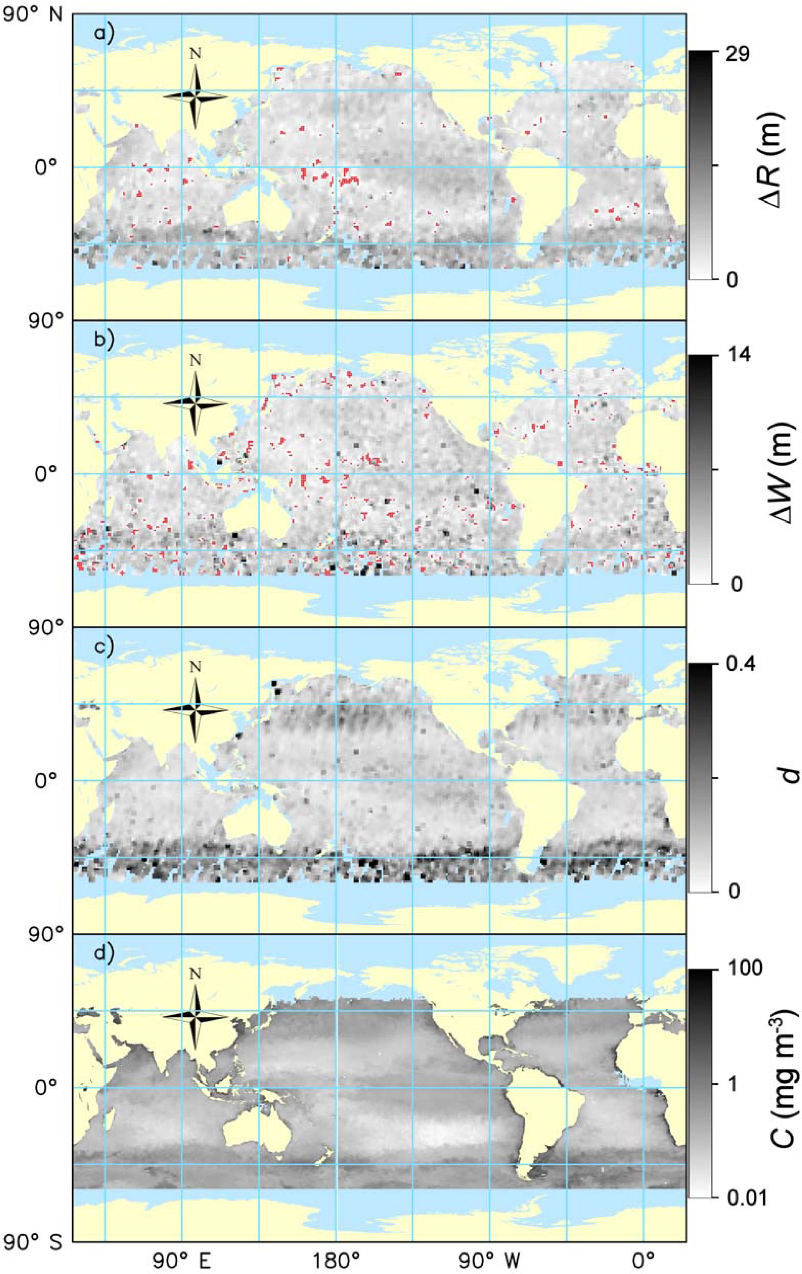
We were also interested in the spatial distribution of the three lidar parameters, ΔR, ΔW, and d(−28). The example of January (Figure 3) presents the parameters after averaging with a 3° filter to make the patterns more visible. There is a rough correspondence between the global patterns of all three of the fitted CALIOP parameters and surface-chlorophyll concentration derived from MODIS data. The highest chlorophyll concentration in January is below 40°S, and this region clearly shows higher values of all three lidar parameters. A region of high chlorophyll above 30°N is clearly seen in the depolarization, is less visible in the range difference, and even less visible in the width difference. The equatorial upwelling zones, which appear as regions of increased chlorophyll concentration, are also seen in the depolarization and range difference, but not it the width difference. There is also a correspondence on smaller scales. Note, for example, the region of higher chlorophyll in the northwest Indian Ocean that is matched by increased range difference and increased depolarization.
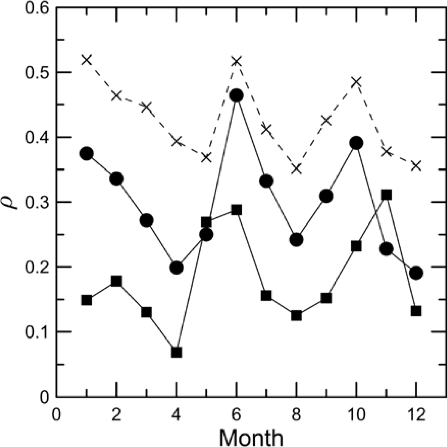
The correlations between monthly averages of all three of the lidar parameters and chlorophyll concentration (Figure 4) are all significant, with statistical p-values < 10−6. The number of data pairs in each of these correlations varies between 6,500 (August) and 19,000 (March), with an average of 11,000. These correlations suggest that phytoplankton might be an important component of the subsurface returns. In restricting the analysis to deep-ocean CALIOP data, we expect that most, although not all, of the data would be from Case 1 waters where the optical properties, including depolarized backscatter, are largely determined by phytoplankton. Bubbles may be present, but would be concentrated near the surface and would not significantly depolarize the lidar return. Concentrations of suspended sediments are generally low away from the coasts. Zooplankton are likely to be present where there are phytoplankton, and these could contribute to the observed correlations. However, we would expect concentrations of zooplankton to be lower than the phytoplankton on which they feed. Particulate organic matter (POM) is also likely to be present where there are phytoplankton, and this could also contribute to the observed correlations. The success of ocean color measurements in measuring chlorophyll concentration in Case 1 waters would suggest that, even if POM is a significant source of backscatter, it can be used to infer chlorophyll.
On the other hand, the correlations are generally <0.5, so the lidar parameters are not completely determined by the near-surface chlorophyll concentration inferred from MODIS. Part of this difference may be related to differences in phytoplankton populations. The depolarization from a phytoplankton cell depends on its size and shape in ways that are unrelated to its chlorophyll content. Part may be related to non-uniform depth distributions of phytoplankton. The presence of subsurface layers will affect remote-sensing reflectance and cross-polarized lidar return differently.
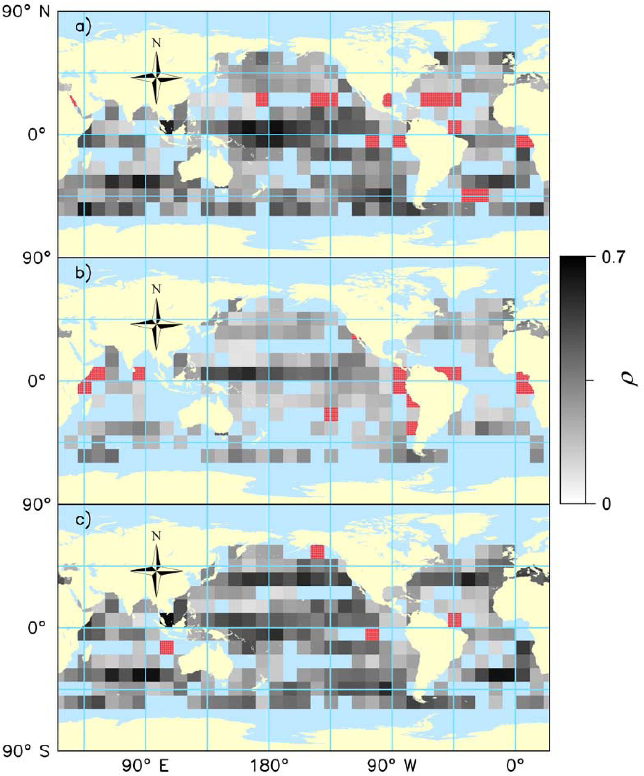
The spatial distribution of these correlations (Figure 5) was calculated using sets of 10° by 10° by 12 month data. There are fewer data pairs used for each correlation in this analysis, ranging from 17 to 905 with an average of 420. The general features of these maps are consistent with the global averages. The depolarization has the highest correlations, with an average of 0.31, and the fewest regions with no significant correlation. Conversely, the width has the most regions with no significant correlation and the lowest average correlation at 0.20. A detailed analysis of the regional differences is beyond the scope of this paper, but there some interesting features. One region that deserves further study is the western tropical Pacific, which has relatively high correlation values. Another is the region from 0°–10°N and 40°–50°W, where all three of the lidar parameters are negatively correlated with chlorophyll concentration and which includes the mouth of the Amazon River. This is consistent with our argument that subsurface returns would not be detectable in waters with high attenuation like the Amazon River plume. Precise determination of how much attenuation could be accommodated is difficult, however, since detection also depends on the level of surface reflection, the amount of subsurface scattering, and the depolarization introduced by that scattering.

3.1. Atmospheric Interference

While the correlations between the lidar parameters and chlorophyll concentration suggest that subsurface scattering is present in the lidar return in addition to the specular surface reflection, it was necessary to rule out the possibility of interference by atmospheric aerosols. That is, depolarization by forward scattering in the atmosphere coupled with a correlation between chlorophyll concentration and AOD might produce correlations between depolarization and chlorophyll concentration that are not representative of subsurface scattering. Note that the question is of depolarization by narrow-angle forward scattering in the atmosphere before or after reflection from the sea surface. This is different from the issue of depolarization by backscattering from non-spherical aerosols, since the return from aerosol backscattering does not contribute to the subsurface signal.
For the small aerosol optical depths used in the analysis, this depolarization can be estimated assuming a single aerosol scattering event. This means that we will consider those photons that are scattered in the forward direction by an aerosol particle and specularly reflected from the sea surface back to the receiver or are specularly reflected from the sea surface and then scattered back to the receiver by an aerosol particle. From symmetry arguments, we can evaluate the aerosol-surface case and use the same result for the surface-aerosol case.
Consider a linearly-polarized beam scattered by an aerosol particle. The scattered field can be expressed in terms of the incident field by the matrix expression,
E s = exp ( ikr ) ikr Q 1 SQ E 0 ,
where Es is the scattered field vector, k is the optical wavenumber, r is the distance to the observation plane, Q is the rotation matrix between the initial plane of polarization and the scattering plane, and S is the scattering matrix. For linearly polarized light, we can let
E 0 = ( E 0 0 ) .
For scattering at an azimuthal angle of φ with respect to the plane of polarization
Q = ( cos ϕ sin ϕ sin ϕ cos ϕ ) .
The scattering matrix for a large, spherical aerosol particle is given by
S = ( S 1 0 0 S 2 ) .
where the scattering amplitudes, S1 and S2, depend on the characteristics of the particle and on the scattering angle. The off-diagonal elements in the scattering matrix are zero for spherical aerosols when the plane of polarization and the scattering plane coincide, and this is the reason for the rotation matrices in Equation (3). The initial coordinate system is rotated into one in which the polarization and scattering planes coincide, the scattering matrix is applied, and then the inverse rotation matrix restores the original coordinate system.
For a distribution of large, spherical aerosol particles, we can assume that S2 = S1cos(θ), where θ is the scattering angle. We will also let cos(θ) = 1 − δ. Because of the receiver field of view (130 μrad), δ will generally be small, but this condition is not required in the following development. Averaging over all azimuthal scattering angles, the cross-polarized irradiance can be expressed as
I X = I 0 8 k 2 r 2 | S 1 | 2 δ 2 .
The scattered irradiance in the co-polarization is
I CO = I 0 8 k 2 r 2 | S 1 | 2 [ 3 + 5 ( 1 δ ) 2 ] .
The depolarization of the scattered light is
d A = I X I CO ,
where the angle brackets denote the average over all scattering angles within the field of view of the lidar and over height. We will approximate the field of view by denoting a maximum δ given by
δ max ( z ) = 1 cos [ tan 1 ( 47 m z ) ] ,
where z is altitude, and the value of 47 m was obtained from the product of the field of view half angle (65 μrad) and the average satellite altitude (720 km). While this maximum value goes to unity at the surface, it is less than 0.1 for z > 100 m.
To illustrate, we can approximate the distribution of scattering angles by the Henyey-Greenstein function [23]
| S 1 ( δ ) | 2 = 1 2 1 g 2 [ ( 1 g ) 2 + 2 g δ ] 3 2 ,
where the asymmetry parameter g is the average value of cos(θ) at the optical wavelength of interest. Winter and Chýlek [24] calculated a value for sea-salt aerosol of g = 0.75. Fiebig and Ogren [25] reported values for g that were generally between 0.58 and 0.64 at one coastal monitoring site and between 0.62 and 0.67 at another. Andrews et al. [26] reported values between 0.59 and 0.72 for “wet” aerosols in Oklahoma. Moorthy et al. [27] reported values between 0.58 and 0.7 over the Indian Ocean. These are not exhaustive, but suggest that the value will generally be somewhere between 0.6 and 0.75 over the ocean.
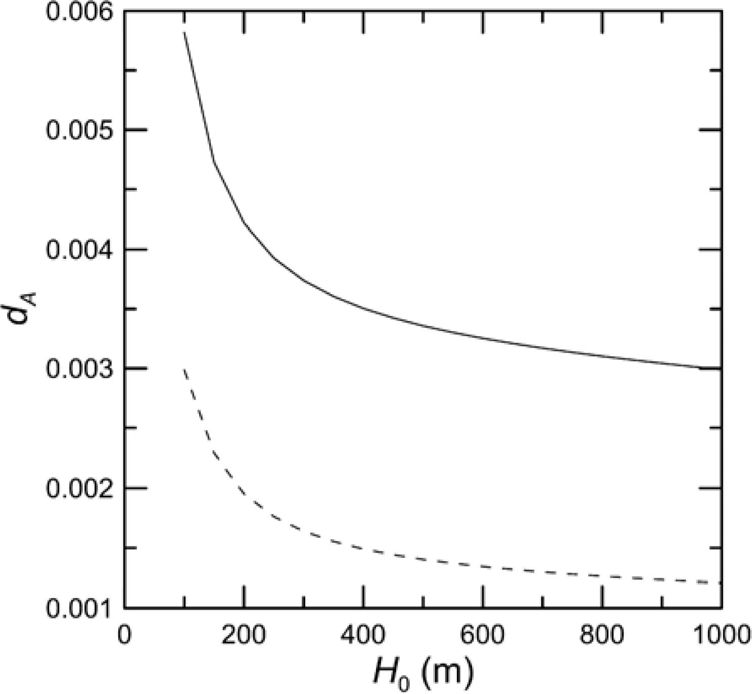
As a first approximation, we will assume that the aerosols are distributed uniformly in height from the surface to some height H0. Figure 6 presents the depolarization for the expected range of g. We conclude that dA is not very sensitive to the vertical distribution of aerosols for heights above 200 m, and that it will almost certainly be less than 0.005 under realistic conditions. Note that this is the depolarization of the scattered light. The aerosol optical depth of the data selected is clustered around 0.05, so only about 10% of the light backscattered from the ocean is also scattered by aerosols during the round trip path through the atmosphere. The actual measured depolarization would then be about a factor of ten less than that of the scattered light, or less than 5 × 10⁻⁴. The average value of the measured depolarization values in the monthly one-degree bins, on the other hand, was 0.036 and only 1.8% of the values were less than ten times the maximum estimated aerosol-induced depolarization. Aerosol scattering, then, does not contribute significantly to the cross-polarized return from the CALIOP data used in this analysis.
As a further check, we recalculated the correlations using only cases with very low winds (<5 m·s−1) and very clear atmospheric conditions (AOD < 0.025). This reduced the number of data pairs in each of the correlation calculations drastically, with the average dropping from 11,000 in the full data set to 2000 in the reduce data set. The correlations between chlorophyll concentration and the three lidar parameters are reduced as a result, but the reductions are relatively small. For d, the change was ρ = 0.43 ± 0.06 to 0.32 ± 0.08 for the average, ± the standard deviation of the 12 monthly values. For ΔR, the change was ρ = 0.30 ± 0.08 to 0.26 ± 0.07 and for ΔW, it was ρ = 0.18 ± 0.08 to 0.13 ± 0.09.

3.2. Receiver Limitations

One limit on the depth to which the CALIOP signal may be attributed to subsurface scattering is the ability to distinguish it from the tail of the impulse response of the photomultipliers used in the 532 nm receivers, and is evident in Figure 1a. The impulse response of each receiver was carefully measured from orbit for both polarizations using land-surface returns collected in 2006 and 2007 [28], and these impulse response functions can be approximated by:
f T = exp [ ( z 15 ) 2 ] + 0.015 exp ( z 118 ) f C = exp [ ( z 15 ) 2 ] + 0.014 exp ( z 110 )
for the total and cross-polarized channels, respectively. Note that z is negative below the surface as in Figure 1a. These functions include both a Gaussian approximation to the effects of the Bessel filter and the exponentially-decaying contribution from signal-induced fluorescence in the photomultipliers [29]. The photomultiplier decay depth of over 100 m is slower than the attenuation of the lidar return in even the clearest waters, since the round-trip attenuation depth would be only about 10 m for pure sea water, which has an attenuation coefficient of 0.05 m−1 at the lidar wavelength. Thus, the temporal response of the photomultiplier will dominate the return at large depths.
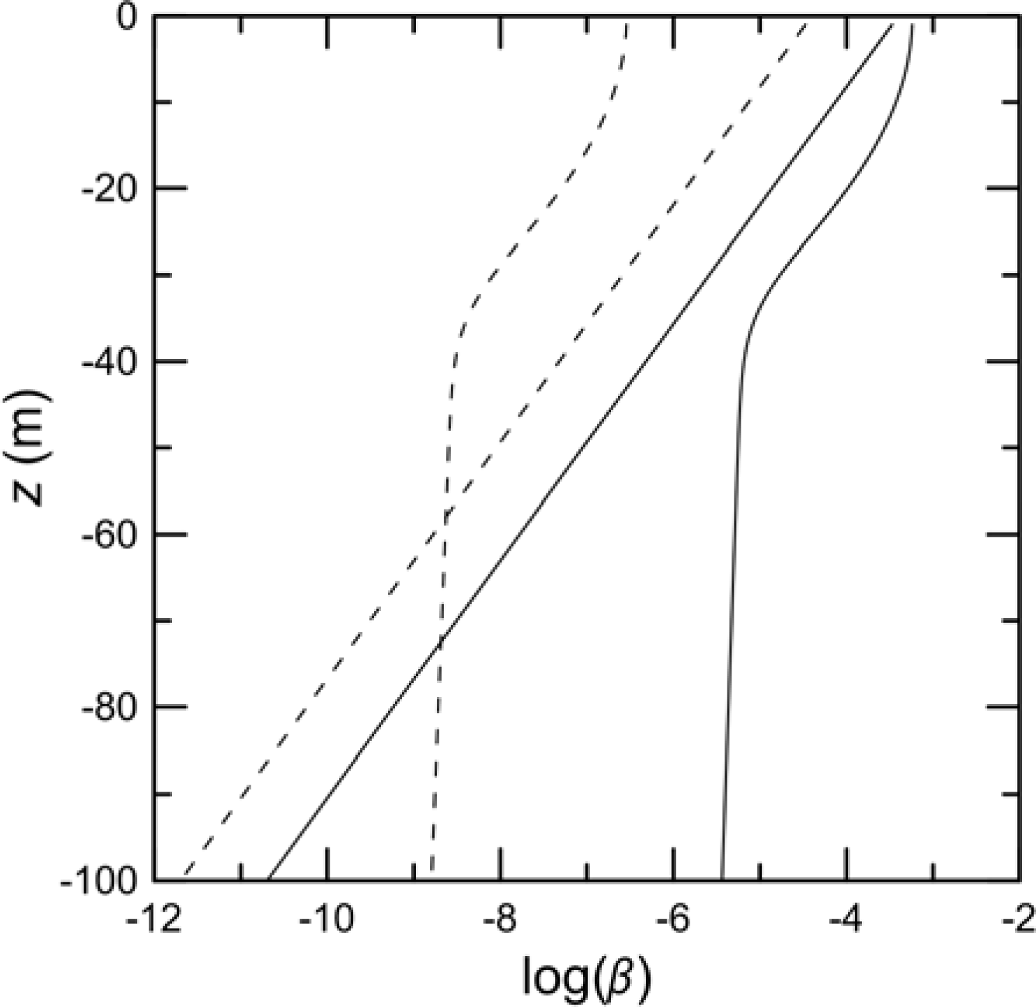
To investigate the limits imposed on depth penetration by the transient response, we considered the following scenario. The attenuated backscatter from the water column from an ideal detector was taken to be
β WT = 3.98 × 10 4 exp ( 0.168 z )
where the water volume backscatter coefficient and attenuation are the average of reported values for pure sea water and clear ocean from the Petzold measurements [30]. The attenuation was calculated from absorption and backscatter using the Lee formula [31,32] for diffuse attenuation coefficient. The corresponding cross-polarized return, βWX, was taken to be 10% of the total return based on clear-ocean measurements with an airborne lidar [19]. The depth profile of the total surface return was taken as
β ST = γ f t dz f t ,
where γ is the integrated surface reflection coefficient from Ref. [15]. Note that there is an error in [15]. The expression for γ in Eqution (3) of that paper is too large by a factor of two. In the example (Figure 7), a wind speed of 10 m·s−1 was used. For the cross-polarized component, βSX, we note that the surface return is a specular reflection that does not create depolarization. This implies that the cross-polarized surface reflection is the result of specular reflection of light that is depolarized by atmospheric aerosols. For this, we assumed a depolarization of 5 × 10⁻⁴ as discussed in Section 3.1.
The water volume returns for ideal detectors and surface returns for the CALIOP detectors are plotted for this case in Figure 7 with the assumption of an ideal receiver with unlimited range resolution. The surface reflection is greater than the volume scattering at all depths for the total return. Enough subsurface scattering to be greater than the surface reflection would require a volume backscattering coefficient typical of very turbid waters. Very turbid waters also have a high attenuation, and only the subsurface scattering very close to the surface could contribute. This would be indistinguishable from the specular surface reflection, so there is no information about subsurface scattering in the total channel. The situation for the cross-polarized return is very different. Here the subsurface scattering is greater than the surface return from the surface to a depth of 58 m. This is fairly robust. This depth decreases, but only to 54 m, if we make conditions much less favorable by halving wind speed, doubling surface depolarization, halving water volume depolarization, or halving water volume backscatter coefficient.
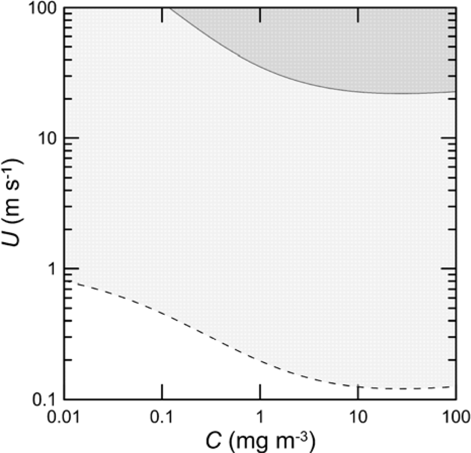
Another way of looking at this issue is to compare the total depth-integrated subsurface return with the surface reflection. For uniform water properties, the total depth-integrated subsurface return is given by
I WT = ψ ( π ) b 2 K D ,
where Ψ is the scattering phase function at a scattering angle of π radians, b is the scattering coefficient, and KD, the diffuse attenuation coefficient, describes the attenuation of the lidar signal for the CALIOP geometry [32]. For the purposes of comparison, we will use simple models based on chlorophyll concentration [33]. At 530 nm, we have
b = 0.311 C 0.62 ,
and
K D = 0.0518 + 0.0467 C 0.67 .
We can separate the scattering coefficient into sea water and particulate contributions and apply the appropriate phase-function values from Petzold [30] to get
I WT = 2.94 × 10 4 + 3.15 × 10 3 ( 0.311 C 0.62 2.5 × 10 3 ) 0.104 + 0.0934 C 0.67 .
To get the corresponding cross-polarized signal, we will assume a constant depolarization of 0.1.
The relationship between the integrated surface reflection and wind from [15] can be inverted to obtain the wind speed at which the surface and subsurface returns would be equal. At wind speeds above this value, we would expect to see a significant return from below the surface. At lower wind speeds, we would not. Figure 8 shows these regimes for the total and cross-polarized signals, assuming a surface depolarization of 0.005. This figure clearly shows that, under most ocean conditions, the total return from the lidar will be dominated by the surface reflection and the cross-polarized return will be dominated by subsurface scattering.

3.3. Examples

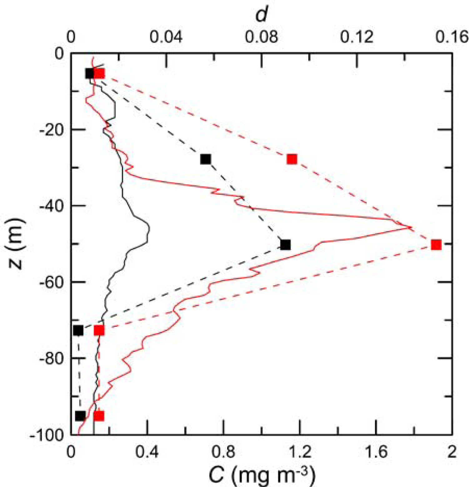
As an example of detection of subsurface scattering layers with CALIOP, we looked for single-shot lidar profiles that, in addition to our other selection criteria, had a depolarization greater than 0.1 at the depth of 50 m. At the lidar depth bin above this, a peak in depolarization can result from the delay and spreading of the near-surface return and does not necessarily imply a peak in scattering. At the depth bin below, the lidar returns can be contaminated by the photomultiplier response. This suggests that the 50 m depth bin is the one most likely to show a clear signature of a subsurface scattering layer. Therefore, we selected two of lidar profiles that were near hydrographic stations reported in the World Ocean Database [34] which included profiles of chlorophyll inferred from fluorescence measurements. The first profile (Figure 9) was taken on 15 July 2010 in the Pacific Ocean 275 km off the coast of California (35.553°N, 124.740°W) on the R/V Point Sur by the US Navy Postgraduate School. The second profile was taken on 28 May 2010 in the Atlantic Ocean 150 km off the coast of Delaware (38.562°N, 73.207°W) on the R/V Delaware II by the Woods Hole Oceanographic Institution under the Ecosystem Monitoring Program (ECOMON). In both cases, there is a maximum in the chlorophyll concentration between 40 and 50 m in depth, which roughly corresponds to the peak in the depolarization. It is interesting that the layer with higher chlorophyll concentration produced more depolarization, but techniques for quantitative retrieval of chlorophyll concentration have yet to be developed.
These examples also provide some insight into the water clarity required to detect layers at depths near 50 m. For the example in the Pacific, the average chlorophyll concentration in the top 30 m was 0.17 mg·m−3. The integrated two-way transmission to this depth, using Equation (17) to estimate the attenuation coefficient at each depth, was 0.019. The example in the Atlantic had an average chlorophyll concentration in the top 30 m of 0.19 mg·m−3 and a two-way transmission of 0.017.

4. Conclusions

The primary conclusion of this study is that subsurface particles can be detected by the CALIOP. Characteristics of the scattering from these particles were shown to be related to chlorophyll concentration near the surface. An increased depolarization (>0.1) at a depth of 50 m was observed under certain conditions. In two examples presented, this depolarization peak corresponds to a peak in the chlorophyll profile, and the example with the higher chlorophyll concentration also had a greater depolarization. This implies that rough profiles of subsurface scattering should be possible to a depth of 50 m. Retrieval of these profiles to infer properties of the water column will require more study.
There are some important limitations, however. The total return is dominated by the strong surface reflection, so useful information will generally only be in the cross-polarized channel. Returns from depths greater than 50 m are not possible under any conditions as a result of the temporal response of the detectors. The correlations are less than unity, so the subsurface scattering is not completely determined by surface chlorophyll. This might be because of changes of chlorophyll concentration with depth and differences in phytoplankton taxa that produce different scattering properties for the same chlorophyll concentration.
The primary effects of subsurface scattering on the broad cross-polarized surface return are a delay of the peak of the return relative to the unpolarized return, a broadening of the temporal pulse, and a depolarization in the return from a nominal depth of 28 m. These are all positively correlated with surface chlorophyll concentration, and are likely to be at least partly a result of scattering by phytoplankton. These correlations are not artifacts of aerosol scattering in the atmosphere and are not artifacts of the temporal response of the detectors. Of the three effects, depolarization seemed to provide the best indicator of subsurface scattering.

Acknowledgments

This work was partially supported by NASA under project number NNH10AO57I. CALIOP data were obtained from NASA Langley Research Center Atmospheric Science Data Center. MODIS AQUA chlorophyll concentrations were obtained from NASA Goddard Space Flight Center. Chlorophyll profiles were provided by the NOAA World Ocean Database. We would like to thank Yongxiang Hu for helpful discussions.

Conflict of Interest

The authors declare no conflict of interest.

References

  1. Brown, E.D.; Churnside, J.H.; Collins, R.L.; Veenstra, T.; Wilson, J.J.; Abnett, K. Remote sensing of capelin and other biological features in the north Pacific using lidar and video technology. ICES J. Mar. Sci 2002, 59, 1120–1130. [Google Scholar]
  2. Churnside, J.H.; Demer, D.A.; Mahmoudi, B. A comparison of lidar and echosounder measurements of fish schools in the Gulf of Mexico. ICES J. Mar. Sci 2003, 60, 147–154. [Google Scholar]
  3. Churnside, J.H.; Thorne, R.E. Comparison of airborne lidar measurements with 420 kHz echo-sounder measurements of zooplankton. Appl. Opt 2005, 44, 5504–5511. [Google Scholar]
  4. Churnside, J.H.; Sharov, A.F.; Richter, R.A. Aerial surveys of fish in estuaries: A case study in Chesapeake Bay. ICES J. Mar. Sci 2011, 68, 239–244. [Google Scholar]
  5. Churnside, J.H.; Brown, E.D.; Parker-Stetter, S.; Horne, J.K.; Hunt, G.L.; Hillgruber, N.; Sigler, M.F.; Vollenweider, J.J. Airborne remote sensing of a biological hot spot in the southeastern Bering Sea. Remote Sens 2011, 3, 621–637. [Google Scholar]
  6. Churnside, J.H.; Donaghay, P.L. Thin scattering layers observed by airborne lidar. ICES J. Mar. Sci 2009, 66, 778–789. [Google Scholar]
  7. Churnside, J.H.; Ostrovsky, L.A. Lidar observation of a strongly nonlinear internal wave train in the Gulf of Alaska. Int. J. Remote Sens 2005, 26, 167–177. [Google Scholar]
  8. Churnside, J.H.; Marchbanks, R.D.; Lee, J.H.; Shaw, J.A.; Weidemann, A.; Donaghay, P.L. Airborne lidar detection and characterization of internal waves in a shallow fjord. J. Appl. Remote Sens 2012, 6, 063611–063615. [Google Scholar]
  9. Krekova, M.M.; Krekov, G.M.; Shamanaev, V.S. Influence of air bubbles in seawater on the formation of lidar returns. J. Atmos. Ocean. Tech 2004, 21, 819–824. [Google Scholar]
  10. Churnside, J.H. Lidar signature from bubbles in the sea. Opt. Express 2010, 18, 8294–8299. [Google Scholar]
  11. Hunt, W.H.; Winker, D.M.; Vaughan, M.A.; Powell, K.A.; Lucker, P.L.; Weimer, C. CALIPSO lidar description and performance assessment. J. Atmos. Ocean. Tech 2009, 26, 1214–1228. [Google Scholar]
  12. Rodier, S.; Zhai, P.; Josset, D.; Hu, Y.; Vaughan, M. CALIPSO Lidar Measurements for Ocean Subsurface Studies. Proceedings of the 34th International Symposium on Remote Sensing of the Environment, Sydney, NSW, Australia, 10–15 April 2011.
  13. Shi, W.; Wang, M. Three-dimensional observations from MODIS and CALIPSO for ocean responses to Cyclone Nargis in the Gulf of Martaban. Geophys. Res. Lett 2008, 35, L21603. [Google Scholar]
  14. Barton, J.S.; Jasinski, M.F. Sensitivity of depth-integrated satellite lidar to subaqueous scattering. Remote Sens 2011, 3, 1492–1515. [Google Scholar]
  15. Hu, Y.; Stamnes, K.; Vaughan, M.; Pelon, J.; Weimer, C.; Wu, D.; Cisewsk, M.; Sun, W.; Yang, P.; Lin, B.; et al. Sea surface wind speed estimation from space-based lidar measurements. Atmos. Chem. Phys. Discuss 2008, 8, 2771–2793. [Google Scholar]
  16. Hu, Y.; Powell, K.; Vaughan, M.; Tepte, C.; Weimer, C.; Beherenfeld, M.; Young, S.; Winker, D.; Hostetler, C.; Hunt, W.; et al. Elevation information in tail (EIT) technique for lidar altimetry. Opt. Express 2007, 15, 14504–14515. [Google Scholar]
  17. Krekov, G.M.; Krekova, M.M.; Shamanaev, V.S. Laser sensing of a subsurface oceanic layer. II. Polarization characteristics of signals. Appl. Opt 1998, 37, 1596–1601. [Google Scholar]
  18. Vasilkov, A.P.; Goldin, Y.A.; Gureev, B.A.; Hoge, F.E.; Swift, R.N.; Wright, C.W. Airborne polarized lidar detection of scattering layers in the ocean. Appl. Opt 2001, 40, 4353–4364. [Google Scholar]
  19. Churnside, J.H. Polarization effects on oceanographic lidar. Opt. Express 2008, 16, 1196–1207. [Google Scholar]
  20. NASA Langley Research Center. CALIPSO Search and Subsetting Web Application. Available online: https://www-calipso.larc.nasa.gov/search/ (accessed on 2 December 2012).
  21. Feldman, G.C.; McClain, C.R. Ocean Color Web, MODIS Reprocessing #3; Kuring, N., Bailey, S.W., Eds.; NASA Goddard Space Flight Center: Greenbelt, MD, USA, 2013; Available online: http://oceancolor.gsfc.nasa.gov/ (accessed on 18 April 2013).
  22. Wentz, F.; Meissner, T. AMSR-E/Aqua Level 2b Global Swath Ocean Products Derived from Wentz Algorithm V002; National Snow and Ice Data Center: Boulder, CO, USA, 2004. [Google Scholar]
  23. Henyey, L.C.; Greenstein, J.L. Diffuse radiation in the galaxy. Astrophys. J 1941, 93, 70–83. [Google Scholar]
  24. Winter, B.; Chýlek, P. Contribution of sea salt aerosol to the planetary clear-sky albedo. Tellus B 1997, 49, 72–79. [Google Scholar]
  25. Fiebig, M.; Ogren, J.A. Retrieval and climatology of the aerosol asymmetry parameter in the NOAA aerosol monitoring network. J. Geophys. Res.-Atmos 2006, 111, D21204. [Google Scholar]
  26. Andrews, E.; Sheridan, P.J.; Fiebig, M.; McComiskey, A.; Ogren, J.A.; Arnott, P.; Covert, D.; Elleman, R.; Gasparini, R.; Collins, D.; et al. Comparison of methods for deriving aerosol asymmetry parameter. J. Geophys. Res.-Atmos 2006, 111, D05S04. [Google Scholar]
  27. Moorthy, K.K.; Nair, V.S.; Babu, S.S.; Satheesh, S.K. Spatial and vertical heterogeneities in aerosol properties over oceanic regions around India: Implications for radiative forcing. Q. J. Roy. Meteor. Soc 2009, 135, 2131–2145. [Google Scholar]
  28. Li, J.; Hu, Y.; Huang, J.; Stamnes, K.; Yi, Y.; Stamnes, S. A new method for retrieval of the extinction coefficient of water clouds by using the tail of the CALIOP signal. Atmos. Chem. Phys. Discuss 2011, 11, 2903–2916. [Google Scholar]
  29. Zhao, Y. Signal-induced fluorescence in photomultipliers in differential absorption lidar systems. Appl. Opt 1999, 38, 1639–4648. [Google Scholar]
  30. Mobley, C.D. Light and Water: Radiative Transfer in Natural Waters; Academic Press: San Diego, CA, USA, 1994; p. 592. [Google Scholar]
  31. Lee, Z.-P.; Darecki, M.; Carder, K.L.; Davis, C.O.; Stramski, D.; Rhea, W.J. Diffuse attenuation coefficient of downwelling irradiance: An evaluation of remote sensing methods. J. Geophys. Res 2005, 110, C02017. [Google Scholar]
  32. Lee, J.H.; Churnside, J.H.; Marchbanks, R.D.; Donaghay, P.L.; Sullivan, J.M. Oceanographic lidar profiles compared with estimates from in situ optical measurements. Appl. Opt 2013, 52, 786–794. [Google Scholar]
  33. Morel, A. Optical modeling of the upper ocean in relation to its biogenous matter content (Case I waters). J. Geophys. Res 1988, 93, 10749–10768. [Google Scholar]
  34. WODselect Maintained by NOAA’s National Oceanographic Data Center. Available online: http://www.nodc.noaa.gov/OC5/SELECT/dbsearch/dbsearch.html (accessed on 14 June 2013).
Figure 1. (a) Typical depth profiles of lidar attenuated backscatter β. Dashed lines connect the values for the total (+) and cross-polarized (×) samples, averaged over 100 shots. Solid lines are the corresponding Gaussian fit to the near surface samples. Red points mark the points where z = R and β = A for each curve and the blue points mark the points where z = R ± W. (b) Depolarization, d, for the same averaged profile.
Remotesensing 05 03457f1
Figure 2. Global average difference between total and cross-polarized range ΔR (solid circles), average difference between total and cross-polarized surface return width ΔW (solid squares), and average depolarization of the first subsurface return at z = −28 m, d(−28) (× connected by dashed line) by month of 2010.
Remotesensing 05 03457f2
Figure 3. Maps of (a) ΔR, (b) ΔW, (c) d(−28), and (d) C for January 2010. Yellow is land, light blue is ocean area with no lidar data. Red points denote negative values.
Remotesensing 05 03457f3
Figure 4. Correlation coefficient ρ between 1° by 1° average chlorophyll concentration, C, and average difference between total and cross-polarized range, ΔR, (solid circles), average difference between total and cross-polarized surface return width, ΔW, (solid squares), and average depolarization of the first subsurface return, d(−28) (× connected by dashed line) by month of 2010.
Remotesensing 05 03457f4
Figure 5. Correlation coefficient ρ between C and (a) ΔR, (b) ΔW, and (c) d(−28) for all months in 10° by 10° regions. Red regions had negative correlations. Light blue regions have latitude > 60° or had no significant (p < 0.05) correlation.
Remotesensing 05 03457f5
Figure 6. Plot of depolarization by atmospheric aerosols, dA, as a function of the surface aerosol layer depth, H0, for asymmetry parameter values of 0.6 (solid line) and 0.75 (dashed line).
Remotesensing 05 03457f6
Figure 7. Depth profiles of lidar attenuated backscatter, β, for volume backscatter using an ideal detector (βWT and βWX, straight lines) and surface reflection using the Cloud-Aerosol Lidar with Orthogonal Polarization (CALIOP) detectors (βST and βSX, curved lines). Solid lines are total return (βWT and βST), and dashed lines are cross-polarized return (βWX and βSX).
Remotesensing 05 03457f7
Figure 8. Wind speed, U, where the integrated subsurface signal will be greater than the integrated surface return for total (above the solid line) and cross-polarized (above the dashed line) channels as functions of chlorophyll concentration, C.
Remotesensing 05 03457f8
Figure 9. Depth profiles of lidar depolarization, d, (squares connected by dashed line) and chlorophyll concentration, C, (lines) from May 2010 in the NW Atlantic Ocean (black) and July 2010 in the NE Pacific (red).
Remotesensing 05 03457f9

