Article

Harmonization of Fraction of Absorbed Photosynthetically Active Radiation (FAPAR) from Sea-ViewingWide Field-of-View Sensor (SeaWiFS) and Medium Resolution Imaging Spectrometer Instrument (MERIS)

Climate Risk Management Unit, Institute for Environment and Sustainability, European Commission Joint Research Centre, TP 272, Ispra 21020, Italy
*
Author to whom correspondence should be addressed.
Remote Sens. 2013, 5(7), 3357-3376; https://doi.org/10.3390/rs5073357
Submission received: 24 May 2013 / Revised: 9 July 2013 / Accepted: 9 July 2013 / Published: 12 July 2013
(This article belongs to the Special Issue High Performance Computing in Remote Sensing)

Abstract

:
This paper describes the combination of terrestrial vegetation observations from two sensors, providing a historical dataset used for an in-depth analysis of the corresponding spatio-temporal patterns. The Fraction of Absorbed Photosynthetically Active Radiation (FAPAR) is an important variable suitable for regional to large-scale monitoring of climate impacts on vegetation. In this work, we create an extensive dataset of FAPAR using a 10-day product at ∼1 km resolution from September, 1997, to April, 2012, combining information from two sensors: the NASA/Sea-viewing Wide Field-of-view Sensor (SeaWiFS) and the European Space Agency (ESA)/Medium Resolution Imaging Spectrometer Instrument (MERIS). The proposed methodology reduces the noise, fills the gaps and corrects for the spurious trends in the data, providing a time-consistent coverage of FAPAR. We develop a fast merging method and evaluate its performance over Europe and the Horn of Africa.

1. Introduction

Earth Observing satellites provide information on the state and evolution of terrestrial vegetation needed to develop and implement environmental policies, to further improve climate change predictions and to assess climate change impacts, adaptations, risk and vulnerability [1].
The analysis of the spatio-temporal patterns of vegetation dynamics, the detection of possible trends in a long time series and the evaluation of their magnitude and statistical significance have always received noticeable interest in geophysical research [25] and even from companies involved in climate risk management [6]. The presence of trends and anomalies may, for example, provide information about the future evolution of the phenology and the impacts of extreme climate events and disturbances on vegetation [710]. The Fraction of Absorbed Photosynthetically Active Radiation (FAPAR) is an Essential Climate Variable (ECV) identified by the Global Climate Observing System [11] that can be monitored from space. This dimensionless variable, varying between zero and one, can monitor the states and changes in the photosynthetic activity of vegetation and, therefore, in phenology. FAPAR is useful to quantify terrestrial vegetation productivity and carbon cycling [12,13]. FAPAR is, thus, useful for many applications, such as agriculture, forestry and environmental monitoring [14]. Optical remote sensing is the most appropriate tool for monitoring FAPAR over vegetated surfaces. The proper interpretation of visible and near-infrared radiation data measured by the sensors relies on the correct understanding and quantification of the solar radiation transfer through the atmosphere and the canopy [15]. Due to the limited lifetime of the satellite instruments, it is not possible to assemble a long time series on the basis of a single sensor, hence the need to combine sensors spanning successive periods. This, however, creates significant challenges to ensure the compatibility and accuracy of these records.
In order to obtain a consistent FAPAR measurement through a longer time, the physical retrieval should be sensor-independent, and the corresponding observations from multiple sensors need to be merged into a continuous time series. This has always been a design criterion for the ESA Joint Research Centre (JRC) algorithm.
Even though SeaWiFS and MERIS products are based on the same ESA JRC algorithm and have been validated against ground-based measurements [1618], because of the inherent differences in the nominal spatial resolution and instantaneous illumination angle at the time of acquisition, the harmonization of the two FAPAR dataset is required.
The key purpose of this paper is to harmonize the observations of FAPAR acquired by SeaWiFS and MERIS, delivering an operationally feasible algorithm that can produce a consistent dataset for the operational vegetation processing data stream. The importance of this merging procedure is amplified in the climate change context, since phenology time series are used to characterize the long-term climate variability and to quantify the ecosystem response to climate and anthropogenic forcing, both at global and local scales. To meet the needs of the monitoring community for a stable long-term FAPAR dataset, we define a simple and efficient harmonization scheme to reduce the slight difference of the FAPAR series from different sensors. The harmonization method presented below implements a three step procedure in which the MERIS and SeaWiFS products are (1) corrected to eliminate remaining noise contamination, (2) gap-filled when fewer than two months are missing and (3) synchronized using two common years of observations. This technique aims to harmonize past and current land surface products and can be extended to future optical sensors, e.g., Advanced Very High Resolution Radiometer (AVHRR), the current one, e.g., Moderate Resolution Imaging Spectroradiometer (MODIS) and Visible Infrared Imaging Radiometer Suite (VIIRS), and future ones, e.g., Ocean and Land Color Instrument (OLCI) on board Sentinel-3 [19]. This procedure can be applied to any type of land surface products, such as surface broadband albedo or Leaf Area Index, on the condition that differences between values derived from various instruments remain reasonably small and synchronized across those sensors.
This paper describes the methodology and presents results with actual data. The method is designed to achieve a globally-representative diverse set of conditions. It will be demonstrated over Europe (25°N–72°N; 32°W–70°W) and over the Horn of Africa (20°N–10°N; 30°W–60°W).

2. JRC-FAPAR Product

Physically-based algorithms suitable to estimate FAPAR, optimized for the data acquired by the Sea-viewing Wide Field-of-view Sensor (SeaWiFS) on board the SeaStar spacecraft and Medium Resolution Imaging Spectrometer Instrument (MERIS) on board the ENVIronmental SATellite (ENVISAT), have been developed at the Joint Research Centre (JRC) [20,21]. These algorithms have been operationally applied at the global scale to the SeaWiFS data collected between September 1997 and June 2006, and to the MERIS data acquired between June, 2002, and April, 2012. These algorithms are designed (1) to provide a high sensitivity to the photosynthetic activity when a vegetated area is detected, (2) to maintain a low sensitivity to soil and atmospheric conditions, (3) to exploit the multi-band specificity of the sensor, (4) to be independent of the geometry of observation and (5) to be platform-independent, thanks to a physical-based approach. In this method, the Fraction of Absorbed Photosynthetically Active Radiation (FAPAR) measured under direct illumination and for a typical ‘green’ leaf has been used for representing the vegetation parameter of interest. Basically, the useful information on the state and evolution of vegetation cover is derived from red and near-infrared spectral band measurements. The blue spectral band, particularly sensitive to aerosols, is ingested to account for atmospheric effects. In practice, the generic FAPAR algorithm implements a two step procedure in which the spectral Bidirectional Reflectance Factors (BRF) measured in the red and near-infrared bands are, first, combined with the information contained in the blue band to optimally achieve decontamination from angular and atmospheric effects and, second, combined together to estimate the FAPAR value (see [16,22] for details).
The FAPAR products used here are re-sampled into grids of 1 km (longitudinal sampling interval = 0.016°, latitudinal sampling interval = 0.011°). The FAPAR time series is originally derived from daily observations captured by SeaWiFS and MERIS at nominal spatial resolutions of 1.5 km and 1.2 km, respectively. For both sensors, a 10-day time composite algorithm was applied in order to composite daily products [23,24]. The time composite algorithm consists in selecting the day over the compositing period (i.e., 10 consecutive days) that corresponds to the most representative FAPAR value of the sequence. Briefly, these representative values are selected, so that they correspond to the closest value to the corresponding arithmetic average of the daily values calculated over that time composite period. The time-composite algorithm, in addition to selecting the ‘most representative day’, also provides the corresponding deviation of FAPAR in the 10-day time series. In addition, the geometry of illumination and viewing angles is provided.
In order to extend measurements through time, multiple sensors with different design and resolution must be merged. To accurately achieve this, the FAPAR time series must be free of noise and trends caused by instrument-to-instrument variability. Gobron et al. [25] already verified the possibility of merging FAPAR records at a global scale with a coarse spatial resolution from MERIS and SeaWiFS sensors.
Validation at nominal spatial resolution for each sensor at a daily scale has been already performed for both sensors in [17,26]: results showed that (1) FAPAR products derived from remote sensing did not deviate from ground-based proxies by more than ±0.1; (2) absolute uncertainties linked to a relative calibration of 3%–4%, are 4%–6%; and, finally, (3) the performance of the optimization is about 0.05 (16%). Each 10-day product has, also, its own temporal deviation derived during the time composite. The average value is of the same order as the total intrinsic accuracy discussed above.
Although each FAPAR algorithm, using sensor-specific formulae and coefficients, minimizes the platform-specific differences, the combination of the FAPAR data series into one continued sequence presents a few problems, due to instrument differences, such as the nominal spatial resolution and the acquisition time. These discrepancies may reduce the accuracy in a downstream application, such as anomaly and/or trend evaluation.
The analysis of the 2002–2004 period, where concurrent observations from SeaWiFS and MERIS are available, reveals a slight discrepancy between FAPAR records. Figure 1 displays the percentage of spatial distribution of the coherency between the SeaWiFS and MERIS FAPAR products, estimated as the percentage of cases when the difference between these products does not exceed the sum of their respective temporal standard deviations. About 4% of the study area over Europe, mostly in the eastern part, is characterized by relatively frequent deviations between the two products. This is probably due to remaining cloud/cloud shadow contamination. The main result is that FAPAR observations from both sensor products agree, within their temporal standard deviation, over more than 60% of the land surfaces, 50% of the time.
Nevertheless, a direct comparison between the 10-day FAPAR product over Europe, acquired in 2003, reveals an average discrepancy, δ, equal to 0.027, and a standard deviation of differences, σ, equal to 0.086 (see top panel of Figure 2). When the same acquisition day has been selected as the representative value for both instruments (not shown here), the standard deviation of differences, σ, is reduced to 0.078. When the same comparison is plot by averaging only valid pixels over a 3 × 3 pixel window, to reduce geo-reprojection problems, the scatter is reduced, but the statistics remain almost the same, except that the correlation coefficient, r, goes from 0.897 to 0.964 and σ decreases up to 0.051.
Comparison between the actual FAPAR products derived by both sensors over Europe and the Horn of Africa (not shown here) reveal a low discrepancy, mostly due to the sensor time acquisition, nominal spatial resolution and remapping errors.

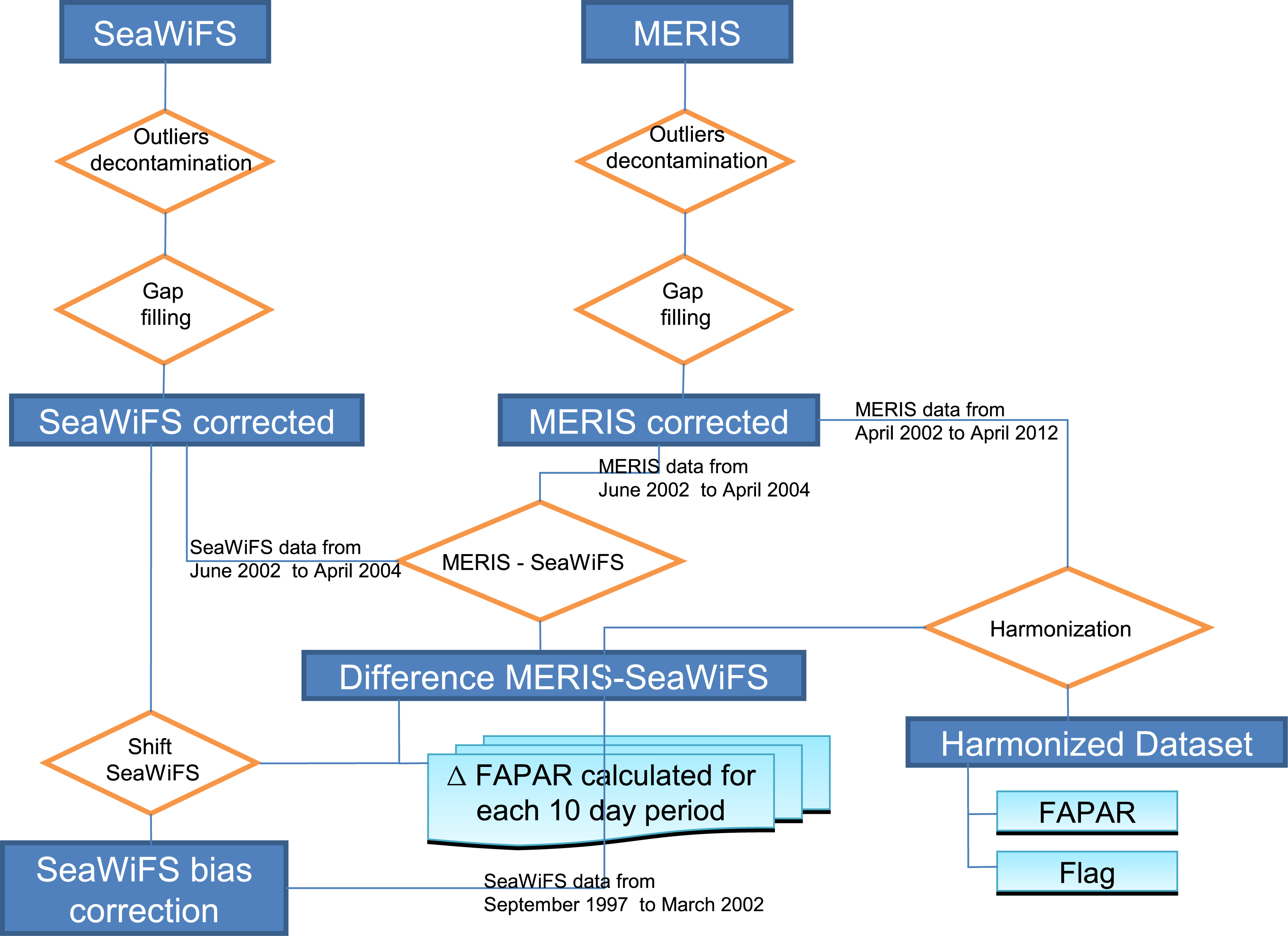
3. Harmonization Method

The proposed methodology to obtain a harmonized dataset is organized through the following steps corresponding to: (1) residual outlier decontamination; (2) gap-filling; and (3) correction of bias. Figure 3 shows the flowchart of the proposed methodology to harmonize the FAPAR product from SeaWiFS and MERIS data. For all practical purposes, both archives are first corrected using ‘residual outliers decontamination’ and gap-filling techniques. The SeaWiFS bias correction is performed using the average differences between the two sensors during the overlap period. Finally, the harmonized FAPAR is retrieved merging the bias corrected SeaWiFS data from September 1997 to May 2002, and the gap-filled MERIS data from June, 2002, to April, 2012, thus selecting MERIS rather than SeaWiFS records when they are both available, in order to keep intact the longer MERIS archive. Further, the quality of records from MERIS is higher than those from SeaWiFS, because of the design and the features of the sensor, such as the push broom, the lower nominal spatial resolution (i.e., 1.2 km vs. 1.5 km) and the data availability. Flags are added to the data, on the pixel basis, to report on the processing steps applied.

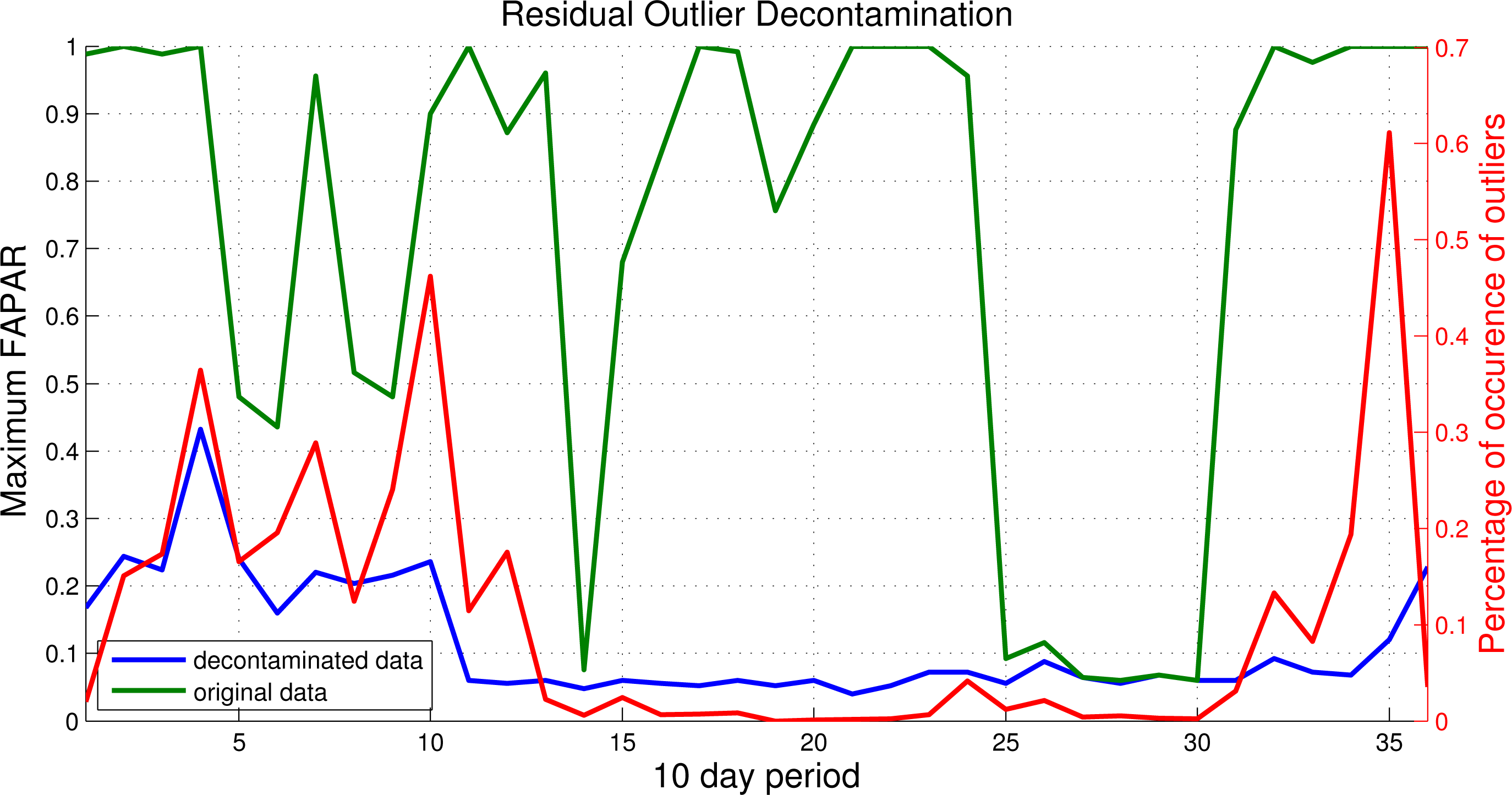
3.1. Residual Outlier Decontamination
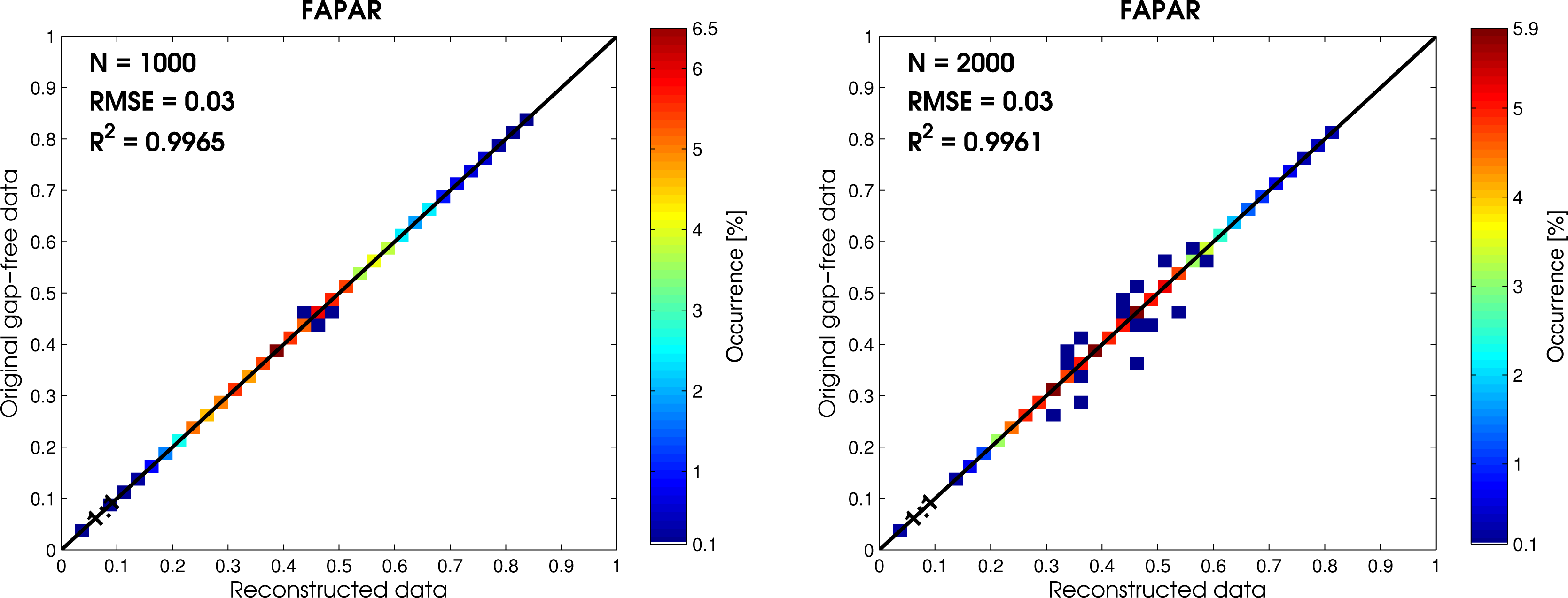
FAPAR daily records, especially over northern Africa, may contain outliers. As the cloud mask in the SeaWiFS processing chain is based only on a threshold algorithm and few acquisitions may be available during each 10-day period, SeaWiFS records may exhibit saturated signals (i.e., close to one) over desert regions. In order to remove these values, a standard mean deviation test is used. The test is performed every year by calculating the mean and the standard deviation of the data and then calling anything that falls more than three standard deviations away from the mean an outlier. This procedure is applied once: the values that are deviating from the natural data variability are rejected and no further iteration is needed. An insight on the need of the residual outlier decontamination is given in Figure 4. Figure 4 displays the time-series of the maximum FAPAR obtained from SeaWiFS for 1998 over a test region located in the Sahara (30°N–35°N, 10°W–10°E) before and after the application of the standard deviation test. Indeed, most of the outliers are found over the desert with SeaWiFS, especially when only one observation occurs (thus making it more difficult to detect by the time-composite procedure). Further, showing the results over a large area, rather than on a single pixel, allows a better representation of the effectiveness of the method (e.g., increasing the occurrence of high FAPAR values). The red line describes the frequency of occurrence of outliers, indicating that the percentage of outliers is always lower than 1%. No significantly saturated signals are observed in the temporal profile of the corrected dataset.

3.1.1. Gap Filling

Surface acquisitions from both sensors are affected by missing data for several reasons, such as the ubiquitous cloud cover and/or the cloud/shadow or snow sub-pixel contamination and the lack of solar illumination at high latitudes. Thus, the gap filling procedure attempts to reduce this problem.
Musial et al. [27] reviewed several temporal interpolations of geophysical time series using smoothing methods, such as splines, Singular Spectrum Analysis and Lomb-Scargle. However, the simplest approach consists in fitting piece-wise linear functions between successive values of the time series (i.e., temporal linear interpolation). Ultimately, this method is chosen for such an application: the purpose of the harmonization is mainly to operationally provide a dataset longer and more consistent than the original one. Users may elect to consider or ignore individual values at the pixel level based on flags that report on the steps implemented. Future work may investigate the opportunity to implement the Eigen Vector Filtering (EVF) method [28] or a spatial and temporal gap-fill, as has been done for soil moisture with the Discrete Cosine Transforms (DCT) [29].
The proposed gap-filling method reconstructs the missing values for each individual grid cell of the temporal domain. A simple linear interpolation is performed over the small gaps, i.e., when the amount of missing data is strictly lower than two consecutive months (i.e., six 10-day periods). The threshold of two months has been selected to avoid creating FAPAR artifacts. However, the gap-filling algorithm is not applied when there are less than ten FAPAR observations per year, i.e., mainly over mountainous regions or at high latitudes.
In order to quantify the effectiveness of this simple methodology, artificial test cases have been designed over a study area, covering an area of approximately 100 km × 100 km, located in the western part of France (51.23°N–52.31°N; 0.72°W–0.90°E). This region has been chosen, because of the low cloud cover occurrence that maximizes the number of cloud-free pixels and reduces the number of ‘natural’ gaps. The test is carried out using FAPAR acquisitions from MERIS during 2006. Synthetic gaps have been introduced into the original dataset, by selecting, in a random manner, 10% of the study area. Then, for each FAPAR time series pertaining to each selected pixel, a continuous period of missing data, varying from one to five 10-day periods, was removed randomly from the series. The gap filling process is then applied to the ‘corrupt’ dataset. Spatially, the window spans over many land cover types; temporally, the gaps can occur at any time during the phenological cycle. The differences between the original values and the corresponding gap-filled estimates are shown in Figure 5, when one (left panel) and two gaps (right panel) occur, which correspond to more than 80% of actual gaps over Europe (66.5% and 20.6%, respectively). The frequency of occurrence of pixels is illustrated by density shading with reddish (bluish) tones illustrating a higher (lower) frequency of occurrence. In addition, the residual distribution shows no significant biases: δ is about 0.001 (0.003) with one (two) gap.

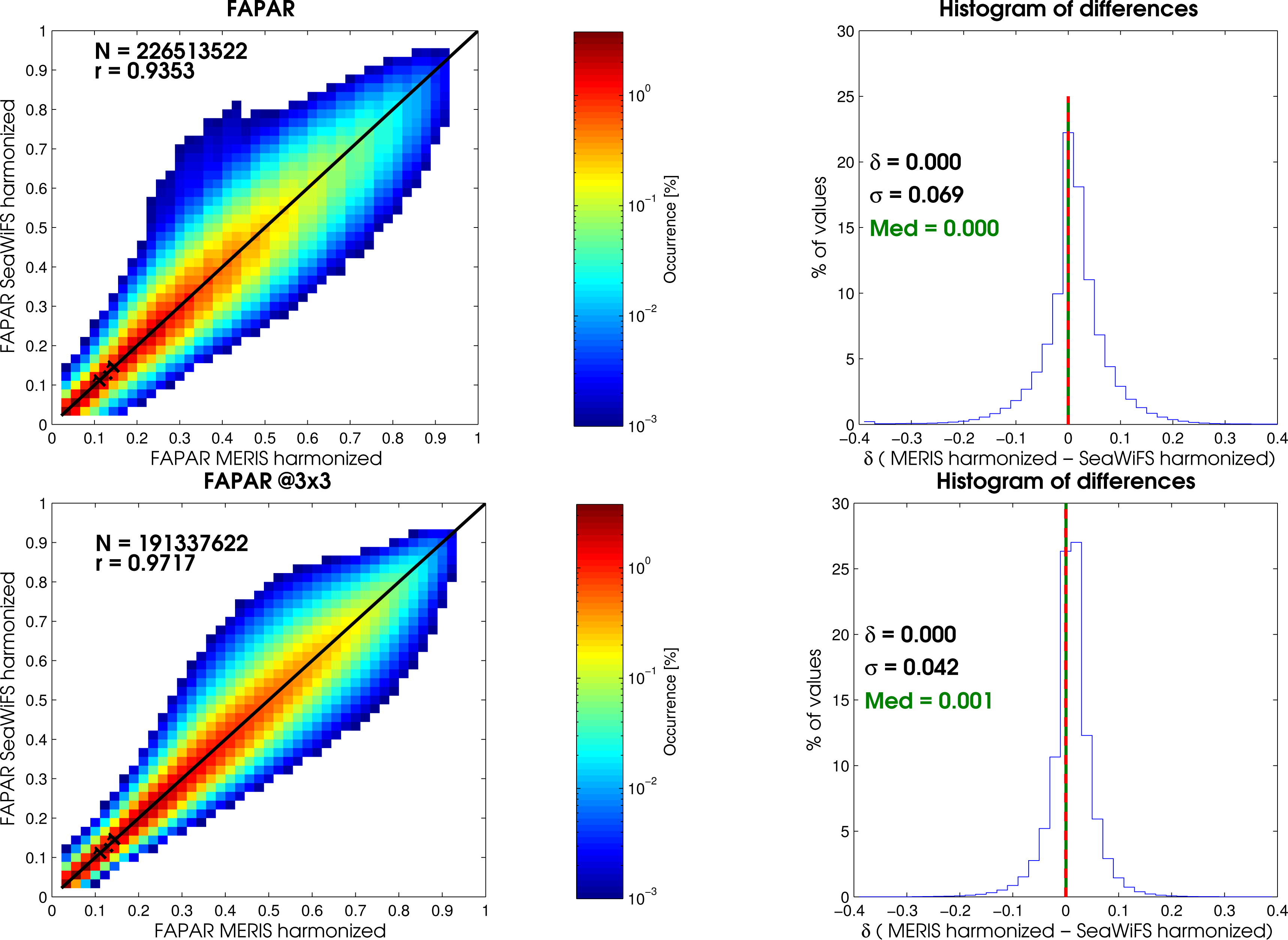
3.1.2. Correction of SeaWiFS Data
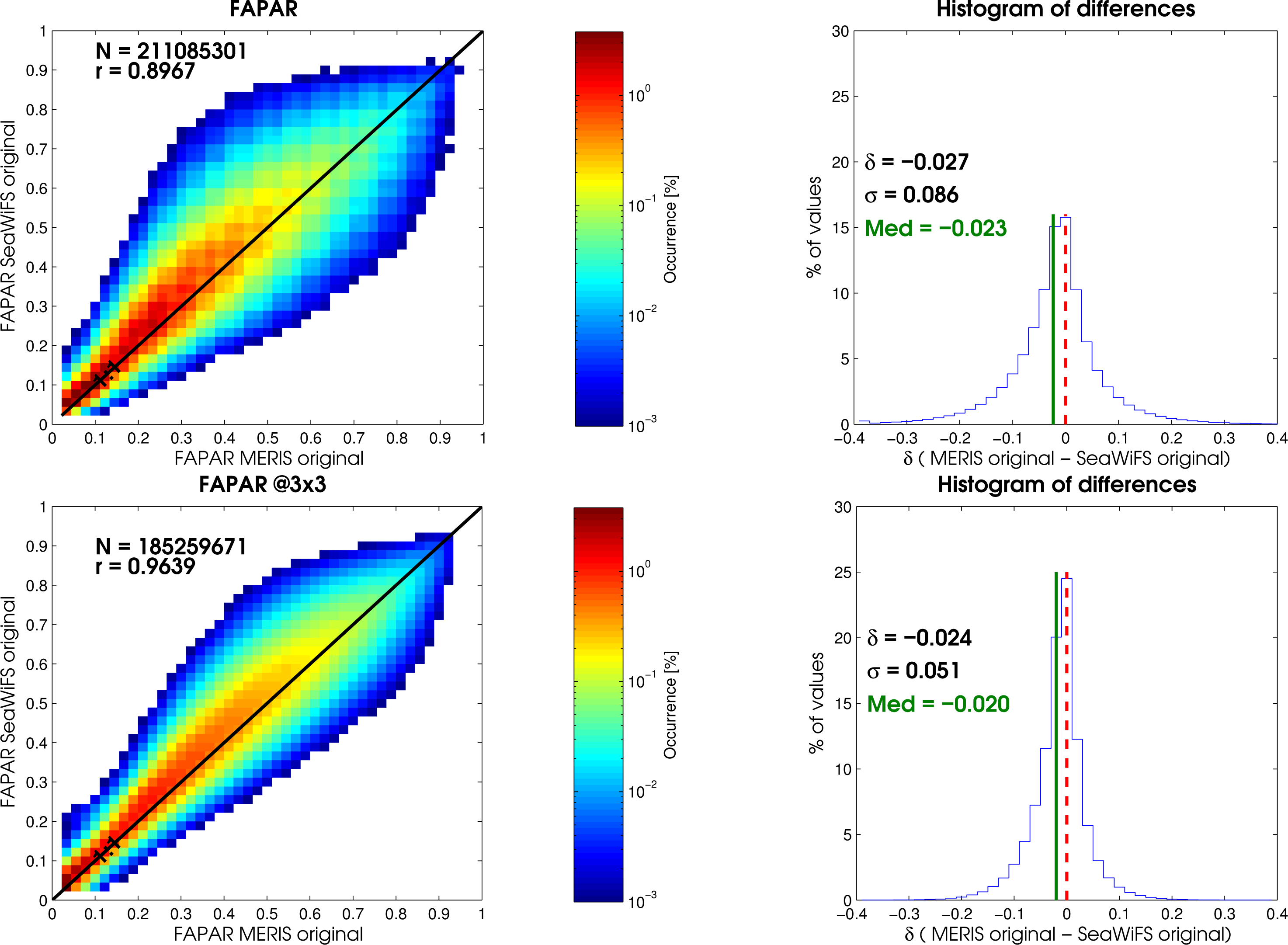
The third step consists in the calculation, for each 10-day period and each individual grid cell, of the average FAPAR difference between MERIS and SeaWiFS from 2002 to 2004. Any individual 10-day difference or average difference score greater than 0.3 is rejected by the bias correction algorithm. Finally, the average 10-day difference is added to the SeaWiFS’ FAPAR time series for each pixel. Note that a difference of 0.3 occurs very rarely, typically less than 0.1% throughout the overlap period. In addition, in 80% of those cases, it is due to the presence of a single observation during the 10-day period, which may be cloud-contaminated.

4. Results

Following the design phase, a test phase was undertaken at each stage of the procedure. The FAPAR distribution was evaluated, and the differences between both sensors were quantitatively compared after each step. The histograms of Figure 6 show that the gap filling does not affect the FAPAR distribution of the whole SeaWiFS time series over 1998–2004 for Europe (top panel) and the Horn of Africa (bottom panel), presenting to what extent the gap filling method is capable of recovering the FAPAR time series.
Figure 7 shows the comparison (scatter-plots and histograms of differences) of the FAPAR 10-day product over Europe acquired in 2003 using harmonized products over the 1 × 1 (top panel) and over the 3 × 3 pixel windows (bottom panel). These scatter-plots are complementary to those of Figure 2, allowing, thus, the comparison between the original and the harmonized datasets. As can be logically expected, Figure 7 illustrates the impact on the harmonization procedure on the FAPAR products, showing the improvement in all statistical indicators. Indeed, the figures show that the harmonization process reduces the averaged value of the differences of FAPAR between MERIS and SeaWiFS (with δ = 0.001). A perfect harmonization would collapse all points on the 1:1 line; it can be seen that the harmonization procedure is particularly efficient, in any case, and the bias is reduced. The correlation coefficient, r, goes from 0.897(0.964) to 0.935(0.972) for 1 × 1 (3 × 3) pixel(s). The proposed methodology supplies a per-pixel flag, informing the processing chain. Each flag documents which procedure was performed (see Table 1) and is, thus, useful for the data analysis and the corresponding applications. For example, the occurrence of Flags 2, 3, 4 and 5 over the two study regions are reported as a function of the year in Figure 8. It is worth noting that ‘only gap-filling’ is mainly applied on the SeaWiFS data; however, it never reaches more then 10% (4%) for the Horn of Africa (Europe) region. This is the case whenever a large proportion of global, rather than local area coverage, SeaWiFS data were used (see [21] for details). The removal of the outliers occurs less than 0.5% of the cases. On average, 96.32% (95.04%) pixels over Europe (the Horn of Africa) have been neither gap-filled nor removed.

5. Impact of Harmonization on Data Series Analysis

With data from both sensors, 14 years of homogeneous records are available to monitor the state and the change of terrestrial vegetation. To test the impact of the harmonization on the time series analysis, we estimate the spatio/temporal variability of the anomalies of FAPAR.

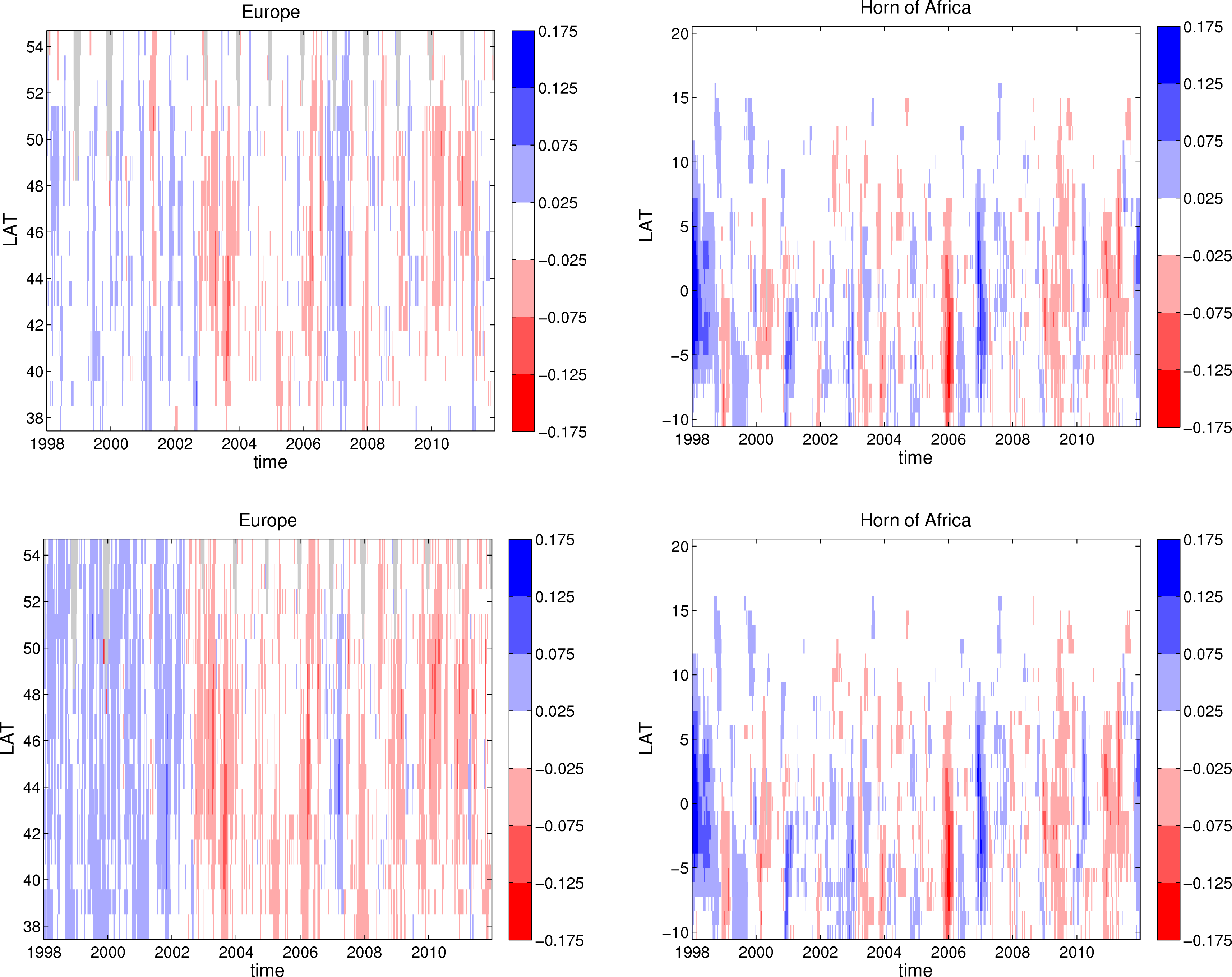
5.1. Spatial Anomalies

Figure 9 illustrates the impact of the harmonization on intense drought analysis, showing the change of anomalous values (see bottom panels) calculated with the original data (top panels) and with the harmonized one (middle panels) over the western part of Europe on 11–20 August 2003 (left panels), and over the Horn of Africa on 1–10 June 2011 (right panels) [3033]. Maps of anomalies coming from both datasets show similar spatial patterns, since the negative anomalies (red color) are dominant compared to the positive ones (blue color). However, the impact of the droughts that struck Europe in the summer of 2003 and the Horn of Africa in 2011 shows a lower signature in the harmonized datasets. Figure 9 indicates that 6.15% (25.67%) of the study area over Western Europe (the Horn of Africa) has an opposite sign to the anomalies, whereas the absolute value of the difference among the anomalies is above 0.05 on 31.22% (8.65%) of the study area.

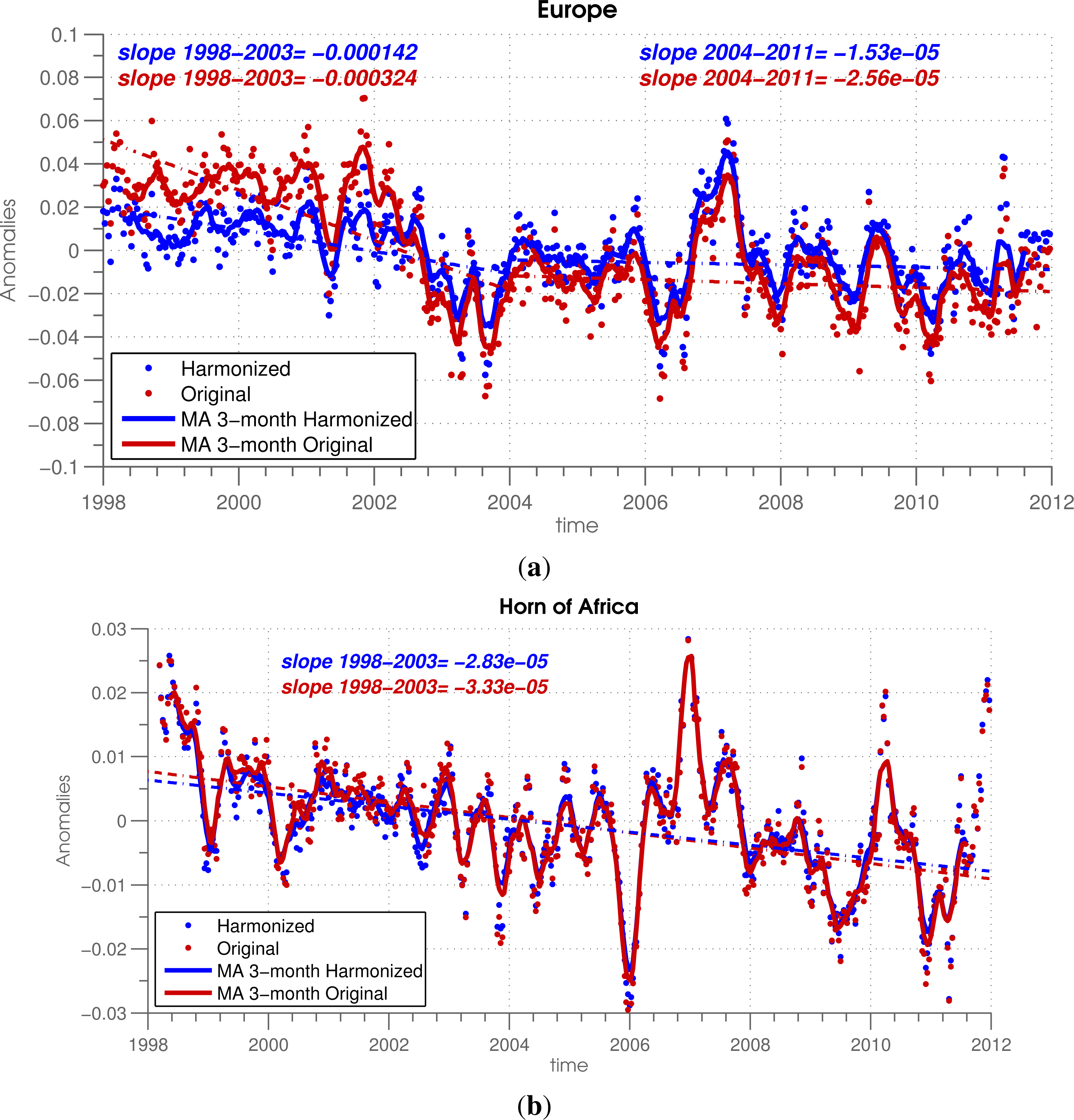
5.2. Temporal Anomalies

Figure 10 focuses on the time evolution of FAPAR signals over local sites with different land cover types. The differences between the three-month moving average anomalies between both datasets generally exhibit temporal variations of up to 0.1 during the first period, i.e., when the SeaWiFs instrument is used, and much reduced after 2003. These differences depend heavily on the site location, and their impacts could be relevant for downstream applications, such as up-scaling in carbon modeling [34]. The dotted (triangle) symbols indicate when at least one value within the three-month period is associated with Flag 2 and 3 (Flag 4 and 5).
Figure 11 displays FAPAR anomalies as a function of latitude, (i.e., the Hovmöller plot) over the Western part of Europe (i.e., within the same spatial domain of Figure 9, right panel) and the Horn of Africa (left panel). With the original dataset (bottom panels), the anomalies’ distribution is rather fluctuating, whereas using the harmonized dataset (top panels), extreme values are smoother. Again, the spatio-temporal patterns of FAPAR anomalies are heavily dependent on the dataset. Over Western Europe, especially before 2002, strong large-scale patterns are mainly due to the differences between instruments’ estimates rather than to a real FAPAR change. It is, however, not the case for the Horn of Africa, where both Hovmöller plots look similar.

5.3. Trends in Temporal Anomalies

The spatial average of anomalies over Western Europe (top panel) and the Horn of Africa (bottom panel) with original and harmonized data are shown in Figure 12. On these figures, the red and blue lines correspond to the use of the original and harmonized product, respectively. Time series of spatially averaged anomalies are different: those calculated with original records tend to be higher in the first period (1997–2002) and lower in the second period (2002–2011), thus creating an apparent trend. Although the corresponding inter-annual variability can be captured by both datasets, their long-term linear trends fitted with the least squares display large differences. The annual linear trends of the anomalies calculated with the original FAPAR are equal to 0.00019 and 0.00003 per 10-day period for the western part of Europe (1998–2003) and the Horn of Africa (1998–2011), respectively. Conversely, the corresponding trends calculated with the harmonized dataset are equal to 0.00005 and 0.00002 per 10-day period, suggesting that the long-term trends of anomalies were overestimated by the original data. These results indicate that the harmonization processing, by correcting the bias between products from both sensors, has a good ability to minimize the artificial trends.

6. Conclusions

This research outlines a simple mathematical approach to monitor the state and changes of terrestrial vegetation using different sensors and to provide a homogeneous, harmonized dataset. SeaWiFS and MERIS are both accurate and versatile instruments to monitor the instantaneous value of the Fraction of Absorbed Photosynthetically Active Radiation (FAPAR), but small differences in spatial resolution and the time of acquisition do not allow a direct combination of their data series into a continuous sequence without undertaking appropriate adjustments. A practical way of incorporating both FAPAR products into a 14 year-long continuum of observations has been presented.
The proposed methodology includes: (1) the removal of outliers over desert surfaces using a 3-sigma test; (2) the reconstruction of missing data with linear interpolation; (3) bias correction on SeaWiFS data; and (4) a flagging strategy to document each step of the procedure. The results were specific to Europe and the Horn of Africa, but the methodology is applicable globally.
The harmonization process over Europe resets the averaged value of the differences of FAPAR between MERIS and SeaWiFS from 0.027 to zero. The utility of the harmonization has been also documented by comparing the spatio-temporal anomalies and trends of FAPAR using the original and the harmonized dataset. The results show that the proposed harmonization strategy minimizes several artificial patterns of anomalies and trends, mainly due to the differences between instruments’ estimates rather than to a real FAPAR change.
The major advantage of this approach presented in this paper lies in its numerical simplicity. The outputs of the procedure also include diagnostic information on each processing step.
The harmonization methodology has been operationally implemented in the Earth Land Information System (ELIS), European facility map server [35].
The outcomes described in this paper open the possibility to extend the FAPAR time series over very long periods from the Advanced Very High Resolution Radiometer (AVHRR) to the future Sentinel-3 sensor [19]. Further applications include the study of the impact of land use changes and droughts on vegetation, carbon budgets and climatic changes.

Acknowledgments

This research was performed in the Climate Risk Management unit of the Institute for Environment and Sustainability at the Joint Research Centre, an institution of the European Commission. The authors thank the providers of the remote sensing dataset needed to perform this research. The SeaWiFS data were obtained from NASA. MERIS 10-day products were processed at the Grid On Demand facility of the European Space Agency (ESA) using JRC codes. The authors acknowledge Michel Verstraete for his help for editing the paper and three anonymous reviewers for their fruitful comments.

Conflict of Interest

The authors declare no conflict of interest.

References

  1. GTOS, Terrestrial Essential Climate Variables for Assessment, Mitigation and Adaptation; GTOS 52; Food and Agriculture Organization, UN: Rome, Italy, 2008.
  2. Moriondo, M.; Giannakopoulos, C.; Bindi, M. Climate change impact assessment: The role of climate extremes in crop yield simulation. Clim. Chang 2011, 104, 679–701. [Google Scholar]
  3. Fischer, E.; Schär, C. Consistent geographical patterns of changes in high-impact European heatwaves. Nat. Geosci 2010, 3, 398–403. [Google Scholar]
  4. Mahecha, M.D.; Fürst, L.M.; Gobron, N.; Lange, H. Identifying multiple spatiotemporal patterns: A refined view on terrestrial photosynthetic activity. Pattern Recognit. Lett 2010, 31, 2309–2317. [Google Scholar]
  5. Wang, K.; Mao, J.; Dickinson, R.E.; Shi, X.; Post, W.M.; Zhu, Z.; Myneni, R.B. Evaluation of CLM4 solar radiation partitioning scheme using remote sensing and site level FPAR datasets. Remote Sens 2013, 5, 2857–2882. [Google Scholar]
  6. Mills, E. Insurance in a climate of change. Science 2005, 309, 1040–1044. [Google Scholar]
  7. Knorr, W.; Gobron, N.; Scholze, M.; Kaminski, T.; Schnur, R.; Pinty, B. Impact of terrestrial biosphere carbon exchanges on the anomalous CO2 increase in 2002–2003. Geophys. Res. Lett. 2007, 34. [Google Scholar] [CrossRef]
  8. Böttcher, H.; Eisbrenner, K.; Fritz, S.; Kindermann, G.; Kraxner, F.; McCallum, I.; Obersteiner, M. An assessment of monitoring requirements and costs of ‘Reduced Emissions from Deforestation and Degradation’. Carbon Balanc. Manag 2009, 4, 7. [Google Scholar] [CrossRef]
  9. Corbera, E.; Schroeder, H. Governing and implementing REDD+. Environ. Sci. Policy 2011, 14, 89–99. [Google Scholar]
  10. Peskett, L.; Schreckenberg, K.; Brown, J. Institutional approaches for carbon financing in the forest sector: Learning lessons for REDD+ from forest carbon projects in Uganda. Environ. Sci. Policy 2011, 14, 216–229. [Google Scholar]
  11. GCOS, Summary Report of the Eleventh Session of the WMO-IOC-UNEP-ICSU; WMO/TD 1189; Rep. GCOS-87; WMO: Melbourne, Australia, 2003.
  12. Running, S.W. Global primary production from terrestrial vegetation: Estimates integrating satellite remote sensing and computer simulation technology. Sci. Total Environ 1986, 56, 233–242. [Google Scholar]
  13. Sellers, P.J.; Dickinson, R.E.; Randall, D.A.; Betts, A.K.; Hall, F.G.; Berry, J.A.; Collatz, G.J.; Denning, A.S.; Mooney, H.A.; Nobre, C.A.; et al. Modeling the exchanges of energy, water, and carbon between continents and the atmosphere. Science 1997, 275, 502–509. [Google Scholar]
  14. Meroni, M.; Marinho, E.; Sghaier, N.; Verstrate, M.M.; Leo, O. Remote sensing based yield estimation in a stochastic framework—Case study of durum wheat in Tunisia. Remote Sens 2013, 5, 539–557. [Google Scholar]
  15. Pinty, B.; Lavergne, T.; Widlowski, J.L.; Gobron, N.; Verstraete, M.M. On the need to observe vegetation canopies in the near-infrared to estimate visible light absorption. Remote Sens. Environ 2008, 113, 10–23. [Google Scholar]
  16. Gobron, N.; Pinty, B.; Verstraete, M.M.; Widlowski, J.L. Advanced spectral algorithm and new vegetation indices optimized for up coming sensors: Development, accuracy and applications. IEEE Trans. Geosci. Remote Sens 2000, 38, 2489–2505. [Google Scholar]
  17. Gobron, N.; Pinty, B.; Aussédat, O.; Chen, J.; Cohen, W.; Fensholt, R.; Gond, V.; Huemmrich, K.; Lavergne, T.; Mélin, F.; et al. Evaluation of fraction of absorbed photosynthetically active radiation products for different canopy radiation transfer regimes: Methodology and results using Joint Research Center products derived from SeaWiFS against ground-based estimations. J. Geophys. Res.-Atmos. 2006, 111. [Google Scholar] [CrossRef]
  18. Gobron, N.; Pinty, B.; Aussédat, O.; Taberner, M.; Faber, O.; Mélin, F.; Lavergne, T.; Robustelli, M.; Snoeij, P. Uncertainty estimates for the FAPAR operational products derived from MERIS-Impact of top-of-atmosphere radiance uncertainties and validation with field data. Remote Sens. Environ 2008, 112, 1871–1883. [Google Scholar]
  19. Donlon, C.; Berruti, B.; Buongiorno, A.; Ferreira, M.H.; Féménias, P.; Frerick, J.; Goryl, P.; Klein, U.; Laur, H.; Mavrocordatos, C.; et al. The Global Monitoring for Environment and Security (GMES) sentinel-3 mission. Remote Sens. Environ 2012, 120, 37–57. [Google Scholar]
  20. Gobron, N.; Pinty, B.; Verstraete, M.M.; Govaerts, Y. The MERIS Global Vegetation Index (MGVI): Description and preliminary application. Int. J. Remote Sens 1999, 20, 1917–1927. [Google Scholar]
  21. Mélin, F.; Steinich, C.; Gobron, N.; Pinty, B.; Verstraete, M. Optimal merging of LAC and GAC data from SeaWiFS. Int. J. Remote Sens 2002, 23, 801–807. [Google Scholar]
  22. Gobron, N.; Ceccherini, G. Multi-Sensor Intercomparison of JRC-FAPAR Products: JRC and VITO Implementation; EUR Report 25668 EN; Publications Office of the European Union: Luxembourg, 2012. [Google Scholar]
  23. Pinty, B.; Gobron, N.; Mélin, F.; Verstraete, M.M. Time Composite Algorithm Theoretical Basis Document; EUR Report 20150 EN; Institute for Environment and Sustainability, European Commission Joint Research Centre: Ispra, Italy, 2002. [Google Scholar]
  24. Aussédat, O.; Gobron, N.; Pinty, B.; Taberner, M. MERIS Level 3 Land Surface Time Composite-Product File Description; EUR Report 22165 EN; Institute for Environment and Sustainability, European Commission Joint Research Centre: Ispra, Italy, 2006. [Google Scholar]
  25. Gobron, N.; Belward, A.; Pinty, B.; Knorr, W. Monitoring biosphere vegetation 1998–2009. Geophys. Res. Lett 2010, 37, L15402. [Google Scholar] [CrossRef]
  26. Gobron, N.; Pinty, B.; Aussédat, O.; Taberner, M.; Faber, O.; Mélin, F.; Lavergne, T.; Robustelli, M.; Snoeij, P. Uncertainty estimates for the FAPAR operational products derived from MERIS-impact of top-of-atmosphere radiance uncertainties and validation with field data. Remote Sens. Environ 2008, 112, 1871–1883. [Google Scholar]
  27. Musial, J.; Verstraete, M.M.; Gobron, N. Comparing the effectiveness of recent algorithms to fill and smooth incomplete and noisy time series. Atmos. Chem. Phys. Discuss 2011, 11, 14259–14308. [Google Scholar]
  28. Ibanez, F.; Conversi, A. Prediction of missing values and detection of ‘exceptional events’ in a chronological planktonic series: A single algorithm. Ecol. Model 2002, 154, 9–23. [Google Scholar]
  29. Wang, G.; Garcia, D.; Liu, Y.; de Jeu, R.; Johannes Dolman, A. A three-dimensional gap filling method for large geophysical datasets: Application to global satellite soil moisture observations. Environ. Model. Softw 2012, 30, 139–142. [Google Scholar]
  30. Schär, C.; Jendritzky, G. Hot news from summer 2003. Nature 2004, 432, 559–560. [Google Scholar]
  31. Gobron, N.; Pinty, B.; Mélin, F.; Taberner, M.; Verstraete, M.M.; Belward, A.S.; Lavergne, T.; Widlowski, J.L. The state of vegetation in europe following the 2003 drought. Int. J. Remote Sens 2005, 26, 2013–2020. [Google Scholar]
  32. Dutra, E.; Magnusson, L.; Wetterhall, F.; Cloke, H.; Balsamo, G.; Boussetta, S.; Pappenberger, F. The 2010–2011 drought in the Horn of Africa in ECMWF reanalysis and seasonal forecast products. Int. J. Climatol. 2012, 33. [Google Scholar] [CrossRef]
  33. Peterson, T.; Stott, P.; Herring, S. Explaining extreme events of 2011 from a climate perspective. Bull. Am. Meteorol. Soc 2012, 93, 1041–1067. [Google Scholar]
  34. Jung, M.; Verstraete, M.; Gobron, N.; Reichstein, M.; Papale, D.; Bondeau, A.; Robustelli, M.; Pinty, B. Diagnostic assessment of European gross primary production. Glob. Chang. Biol 2008, 14, 2349–2364. [Google Scholar]
  35. Institute for Environment and Sustainability, European Commission Joint Research Centre. Earth Land Information System (ELIS). Available online: http://fapar.jrc.ec.europa.eu (accessed on 6 May 2013).
Figure 1. Percentage of spatial distribution of the coherency between the Sea-viewing Wide Field-of-view Sensor (SeaWiFS) and Medium Resolution Imaging Spectrometer Instrument (MERIS) Fraction of Absorbed Photosynthetically Active Radiation (FAPAR) products, estimated as the percentage of cases when the difference between these products does not exceed the sum of their respective temporal standard deviations.
Remotesensing 05 03357f1
Figure 2. Scatter-plots and histograms of the differences of the FAPAR 10-day product over Europe acquired in 2003 using MERIS and SeaWiFS products over a 1 × 1 pixel (top) and 3 × 3 pixel window (bottom). Reddish (bluish) areas in the plots indicate a higher (lower) density of sample points. The 1:1 line is shown in black.
Remotesensing 05 03357f2
Figure 3. Flow chart of the harmonization procedure.
Remotesensing 05 03357f3
Figure 4. Example of the residual outlier decontamination: plot of the maximum FAPAR over a target area (box 30°N–35°N,10°W–10°E) in 1998. The plot of maximum FAPAR values over the target area before the application of the standard deviation test (green line) emphasizes the presence of outliers at each time step (i.e., 10-day period). Replicating the same analysis after the 3-sigma test (blue line) reveals that saturated signals have been removed. The red line represents the frequency of outliers.
Remotesensing 05 03357f4
Figure 5. Impact of the gap filling process on the FAPAR dataset over a test region located in the western part of France. Scatterplot of observed and reconstructed FAPAR fields from MERIS during 2006 with one gap (left panel) and with two consecutive gaps (right panel). The underlying idea of this test is to use an almost cloud-free FAPAR time series representing the ‘truth’, to alter them by imposing data gaps randomly and to evaluate the performance of the temporal gap-filling approach described above.
Remotesensing 05 03357f5
Figure 6. FAPAR distribution from SeaWiFs records (i.e., 1998–2004) before (blue bars) and after (red bars) gap filling over Europe (a) and over the Horn of Africa (b).
Remotesensing 05 03357f6
Figure 7. Scatter-plots and histograms of the differences of the FAPAR 10-day product over Europe acquired in 2003 using harmonized products over the 1 × 1 pixel (top panel) and over the 3 × 3 pixel window (bottom panel).
Remotesensing 05 03357f7
Figure 8. Frequency of Flag 2 and Flag 3 (i.e., only the gap filling is applied) and Flag 4 and Flag 5 (i.e., both the gap filling and the outlier decontamination are applied) occurrences over Europe (green bars) and over the Horn of Africa (orange bars).
Remotesensing 05 03357f8
Figure 9. Anomalies of FAPAR calculated with the original (top) and harmonized (middle) products and differences (bottom) over the western part of Europe August 11–20, 2003 (left), and over the Horn of Africa June 1–10, 2011 (right).
Remotesensing 05 03357f9
Figure 10. Differences between three-month moving average anomalies over local sites with different land use using the original and the harmonized dataset.
Remotesensing 05 03357f10
Figure 11. Hovmöller plots of the FAPAR anomalies over Western Europe (left) and over the Horn of Africa (right), employing the harmonized (top) and the original (bottom) products. Positive (negative) anomalies, corresponding to values greater (lower) than the 14-year mean are displayed in bluish (reddish) tones. Periods with no FAPAR data are plotted as grey areas.
Remotesensing 05 03357f11
Figure 12. Differences between the anomalies calculated with the original data (red line) and with the harmonized data (blue line) over Western Europe (a) and over the Horn of Africa (b).
Remotesensing 05 03357f12
Table 1. Meaning of flag for the harmonized FAPAR product.
Outlier DecontaminationGap-FillingBias CorrectionFlag
NoNoNo0
NoNoYes1
NoYesNo2
NoYesYes3
YesYesNo4
YesYesYes5

