Removal of Optically Thick Clouds from Multi-Spectral Satellite Images Using Multi-Frequency SAR Data

Abstract

This study presents a method for the reconstruction of pixels contaminated by optical thick clouds in multi-spectral Landsat images using multi-frequency SAR data. A number of reconstruction techniques have already been proposed in the scientific literature. However, all of the existing techniques have certain limitations. In order to overcome these limitations, we expose the Closest Spectral Fit (CSF) method proposed by Meng et al. to a new, synergistic approach using optical and SAR data. Therefore, the term Closest Feature Vector (CFV) is introduced. The technique facilitates an elegant way to avoid radiometric distortions in the course of image reconstruction. Furthermore the cloud cover removal is independent from underlying land cover types and assumptions on seasonality, etc. The methodology is applied to mono-temporal, multi-frequency SAR data from TerraSAR-X (X-Band), ERS (C-Band) and ALOS Palsar (L-Band). This represents a way of thinking about Radar data not as foreign, but as additional data source in multi-spectral remote sensing. For the assessment of the image restoration performance, an experimental framework is established and a statistical evaluation protocol is designed. The results show the potential of a synergistic usage of multi-spectral and SAR data to overcome the loss of data due to cloud cover.

1. Introduction

Recent advances in remote sensing are providing numerous opportunities in almost every branch of environmental research. The civil fields of application for multi-spectral remote sensing instruments in Earth observation are diverse, spanning from the monitoring of forests, oceans or urban areas over agricultural applications to the exploration of natural resources, etc. A major prerequisite for a sufficient analysis of Earth observation data is the provision of information that is free from external influences and disturbances [1,2]. One possible cause of data gaps is cloud cover. Cloud cover is recognized as a source of significant loss of information and data quality by many scientific studies [3–7]. The existence of clouds hinders the extraction of meaningful information because they are a considerable source of uncertainty with regard to the application of any algorithm aiming at the retrieval of land surface parameters. In order to overcome the problem of cloud cover in Earth observation data, the reconstruction of areas beneath clouds can be regarded as a fundamental research topic, especially concerning the visible and infrared regions of the electromagnetic spectrum. With the growing availability of multi-spectral, hyperspectral and microwave satellite sensors, opportunities for the analysis of complementary data sources arise. Therefore the task of reconstruction of cloud-obscured pixels in multi-spectral images may be regarded as an issue of synergy between these complementary sources.

2. Removal of Optical Thick Clouds

In this study the removal of optical thick clouds from multi-spectral images is conducted. In this case the information beneath the cloud is not accessible by multi-spectral image sensors. Therefore the areas obscured by cloud cover can be regarded as No Data and must be reconstructed by additional data sources. Existing methods for the removal of optically thick cloud can be categorized into substitution and interpolation techniques.

2.1. Substitution Techniques

Substitution is a very simple way of cloud cover removal. In general a pixel identified as cloudy is simply replaced by the digital numbers (DN) of a pixel at the same location of another image of the same sensor [8]. Because of significant differences between the DN of a pixel between two image acquisitions, some calibrations and corrections are mandatory for cloud substitution. These differences originate from factors like atmospheric conditions, sun-target-sensor geometry, sensor calibration, soil moisture or vegetation phenology [4]. The signal attenuation due to atmospheric distortions has to be corrected image-wise to consider the specific conditions during image acquisition [9,10]. In order to account for the sun-target-sensor geometry, topographic normalization can be applied to reduce spectral reflectance differences that occur due to the influence of terrain slope and aspect [11]. Although the reflectances of the images contributing to the cloud-free mosaic were corrected in two ways, the occurrence of different reflectances is still possible. Therefore the differences in the mean reflectance level between the cloudy image and the cloud-free fill image have to be reduced [12]. The advantage of substitution techniques is the simplicity of the used algorithms, since a pixel value is replaced by the corresponding DN of another image from the same sensor. Hence, complex interpolation techniques are not necessary here and issues due to the usage of different sensors can be neglected. A drawback of these techniques is the number of potential error sources in the preprocessing chain due to the high number of the aforementioned steps. The most significant shortcoming, however, is that temporal differences, for example land cover change, between the images are often completely neglected (e.g., [13]).

2.2. Interpolation Techniques

The interpolation of pixels obscured by cloud cover can be regarded as an approximation of unknown values within an arrangement of known values [14]. By this definition it is obvious that missing values are reconstructed by analyzing a certain number of measurements to infer the value of a missing measurement. Interpolation can be accomplished in the temporal or in the spatial domain. The interpolation of time series to reconstruct cloudy pixels is mainly based on index composites like the normalized difference vegetation index (NDVI), gross primary production (GPP) or net primary production (NPP) [15]. The basic concept is the identification of outliers with respect to the time series and their replacement with estimated values of a certain model [5]. Cihlar and Howarth [3] present an approach for the correction of NDVI time series with respect to this method. Based on the assumption that the NDVI of a cloud obscured pixel is lower than the NDVI of a cloud-free pixel—since atmospheric attenuation decreases the contrast between the VIS and the NIR parts of the EM-spectrum—and the assumption that a time series of NDVI composites will have a significant seasonal behavior, missing values can be reconstructed. The interpolation in the spatial domain is based on the general assumption that variability within an image is spatially dependent. In other words, neighboring pixels are more likely to be similar to each other than pixels in greater distances [16–19]. Therefore the spatial structure of a cloudy image as well as the spatial cross correlation with a secondary cloud-free image can be employed to reconstruct cloud affected pixels [19]. The estimation of the DN values based on these assumptions can be carried out in several manners, for example with geostatistical interpolation methods like Cokriging (Ibid.). Other techniques are based on contextual approaches. For example, Melgani [20] employs a model for the estimation of a DN of a cloudy pixel, which is trained first with spatial and temporal information of adjacent regions in order to create context-based rules for the reconstruction of the cloudy pixel.

3. The Need for More Generic Data Restoration Strategies

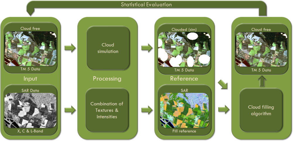
Most of the applied methods for image restoration beneath clouds suffer from certain major drawbacks. Simple substitution or compositing techniques either assume that no significant land cover changes between the time step of the image to be reconstructed and the time step of the image used for reconstruction have happened or they simply ignore temporal offsets entirely [21]. Furthermore, a completely cloud-free image cannot be guaranteed since certain pixels may be obscured by cloud cover in all images the composite is based on. Additionally, the image-wise correction of atmospheric conditions as well as radiometric differences between images is a challenging task and must be accomplished first. Interpolation over time requires a high temporal resolution and a sufficient length of the image acquisition period to cover seasonal aspects. The interpolation methods mentioned in Section 2.2 are restricted in terms of sensor type and/or ground cover type and depend on the cloud type [20]. Therefore, more generic approaches are necessary to restore the image information beneath clouds.

To overcome the drawbacks of the existing algorithms, it is not necessarily required to come up with fundamentally new and complex image processing algorithms. The key to a reliable method to restore missing image information in general, and more specifically to remove cloud cover, might be already provided by existing data and technology. A straightforward combination of complementary data and meaningful algorithms is a possible solution to restore error-affected satellite images in a more suitable way. The essential step to accomplish this objective is to take into account the complementary nature of data sources like multi-spectral and SAR data. Intuitively, the differences between the image acquisition processes, the underlying physics and the differing imaging geometry appear to be an obstacle for the synergistic combination of these two data sources. However, by taking a closer look, the synergetic potential becomes obvious. Both multi-spectral and SAR data rely on interactions of electromagnetic radiation with the Earth’s surface. Based on this premise it seems reasonable to investigate the synergetic potential of these data sources to fill data gaps as shown by [22]. Figure 1 demonstrates the plausibility of this hypothesis. Comparing a single SAR band (e.g., L-HH) to a multi-spectral RGB image, the separability between the features is very poor, especially for agricultural areas. However, by combining different frequency bands (e.g., X-HH|X-HV|L-HH) to a color composite, the strong relation between visible/near-infrared (VIS/NIR) and microwave information becomes obvious.

Therefore, this study combines multi-spectral and SAR satellite images to reconstruct cloud affected areas in the multi-spectral images. On the way to a meaningful technology aiming for the mentioned goal, it is mandatory to be able to evaluate the quality of the image reconstruction results. Therefore a complete framework for image reconstruction and quality estimation was implemented (Figure 2), comprising cloud cover simulation, image restoration and statistical evaluation of the differences between the original cloud-free image and the associated restoration result. In the following the individual modules of Figure 2 are described in detail.

4. Data and Methods

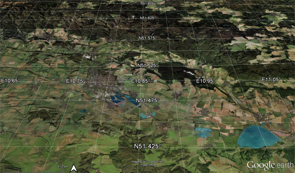
4.1. Investigation Area and Data

The basin area “Goldene Aue” near Nordhausen is located in the transition zone between the Federal State of Thuringia and Saxony-Anhalt in the Federal Republic of Germany (Figure 3). It is margined by the mountain ranges “Harz” in the North, “Windleite” in the South and “Kyffhäuser” in the Southeast. These ridges are characterized by forested areas. The interjacent basin area is characterized by intense agricultural usage. This vast heterogeneity and structural complexity qualify the “Goldene Aue” as an optimal test site for the experimental image reconstruction.

The data basis used in this study comprises two types of input data. On the one hand, multi-spectral satellite imagery from the sensors Landsat and SPOT 4 is employed. On the other hand, SAR satellite imagery from the sensors TerraSAR-X (TSX), ERS and PALSAR (ALOS) is used. The preprocessing of the multi-spectral imagery was restricted to the resampling of the SPOT scene to the Landsat resolution of 30 m and the respective coregistration of the images.

Table 1. Overview of the multi-spectral data used in this study.

Property	Landsat TM 5	SPOT 4
Acquisition Date	2010-07-08	2010-07-09
Original Resolution	30 m	20 m
Final Resolution	30 m	30 m
Spectral Bands (μm)	Blue (0.45–0.52)
	Green (0.52–0.60)	Green (0.50–0.59)
	Red (0.63–0.69)	Red (0.61–0.68)
	NIR (0.76–0.90)	NIR (0.78–0.89)
	SWIR-1 (1.55–1.75)	SWIR (1.58–1.75)
	Thermal (10.4–12.5)
	SWIR-2 (2.08–2.35)

gives an overview of the properties of the multi-spectral imagery used in this study. For the sake of complexity reduction, all SAR data are processed to a resolution of 30 m. The advantages of this approach are the comparability with the Landsat image in terms of spatial resolution and the exclusion of spatial resolution as a variable of the resulting cloud fill quality.

Table 2. Overview of the SAR data used in this study.

Property	TSX	ERS	ALOS
Acquisition Date	2010-07-10	2010-06-09	2010-07-09
Acquisition Mode	SM *	IM **	FBD ***
Polarization State	HH/HV	VV	HH/HV
Incidence Angle	22.13°	23.18°	38.74°
Band Name	X-Band	C-Band	L-Band
Frequency	9.6 GHz	5.3 GHz	1.27 GHz
Wavelength	3 cm	5.6 cm	23.6 cm
Pass Direction	Descending	Ascending	Ascending
Looking Direction	Right	Right	Right
R+/A++ Resolution	4.22 m/4.39 m	20.01 m/19.85 m	15.2 m/12.53 m
R/A ML+++-Factor	12/12	1/5	2/8
Original Resolution	1.1 +/2.4 ++ m	3.9 +/7.9 ++ m	9.3 +/3.1 ++ m
Final Resolution	30 m	30 m	30 m

^*SM—StripMap;

^**IM—Image Mode;

^***FBD—Fine Beam Dual;

⁺R—Range Direction;

^A++—Azimuth Direction;

^ML+++—Multilooking.

gives an overview of the SAR data and related processing parameters applied to them.

4.2. Methodological Considerations and Requirements

To achieve the mentioned objectives, certain fundamental assumptions are mandatory. The most essential step towards a successful cloud removal is their detection [23]. Within this study, the cloud detection is regarded as given, since the work was not supposed to focus on cloud detection algorithms. Hence, cloud cover was simulated in the framework of this study. Detailed disquisitions of this topic are beyond the scope of this paper. Furthermore, cloud shadows were neglected completely. This assumption is justified by the abstraction of clouds (and their shadows) to areas of no information. Moreover, this study is focused on the removal of optically thick clouds with no contribution of the ground beneath a cloud to the signal received at a sensor. Therefore all evaluations are based on the consideration of small, optically thick fair weather cumulus clouds.

Based on these assumptions, the following methodological requirements arise for the framework of this study:

• Implementation of a generic pixel-based cloud removal algorithm as a step towards the compensation of the drawbacks of substitution and interpolation techniques. The algorithm is supposed to be:

  • ○ sensor independent,
  • ○ based on physical interrelations,
  • ○ independent from the land cover,
  • ○ methodologically simple, and
  • ○ generating reproducible outputs;
• Establishment of a framework for the statistical evaluation of the performance of the cloud cover removal algorithm;
• Evaluation of the potential of mono-temporal, multi-frequency SAR imagery to serve as data basis for the image restoration of a multi-spectral image.

To achieve the abovementioned objectives, certain basic requirements on data and methodology can be inferred. In order to consider land cover change as negligible, it is mandatory to include data with very short temporal baselines in relation to the cloud obscured multi-spectral image. Another data related premise is the endeavor to keep the demand for cloud-free reference data as minimal as possible but to include as much data as necessary. On the methodological side, it is desirable to reduce the complexity of the algorithm as much as possible. In order to achieve a logical intuitive restoration of missing information, the number of variables should be minimized. The inner assembling of the algorithm is supposed to be a white box system, i.e., the structure and functionality must be known and a certain input produces always the same output. Furthermore, the framework for the evaluation of image restoration performance is supposed to be able to quantify the quality of the reconstruction. Therefore, objective statistical measures seem expedient to minimize the demand for subjective criteria such as visual comparison.

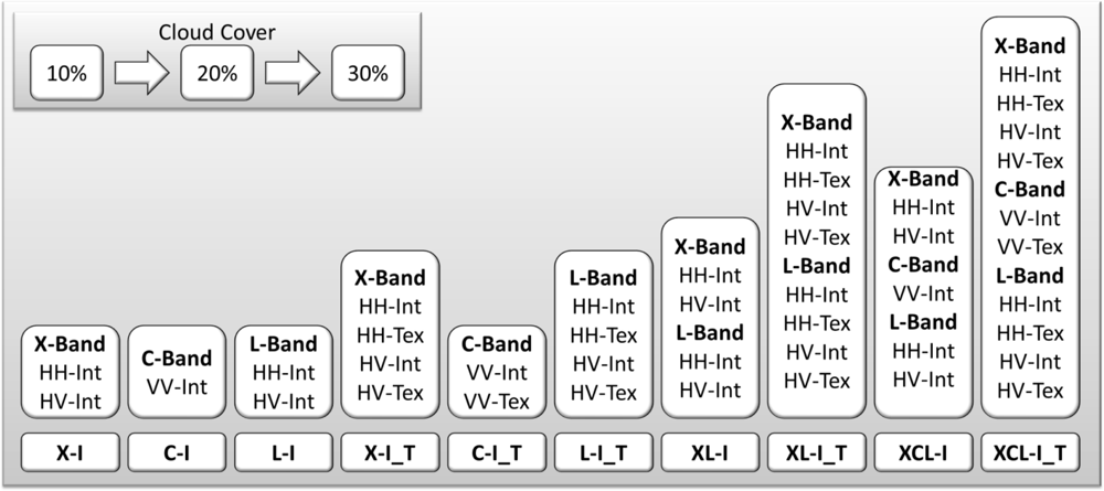
4.3. Cloud Simulation

The simulation of cloud cover is one of the two major steps within this study. For the sake of comparability, simulated cloud cover in multi-spectral imagery has numerous advantages. Besides the opportunity to evaluate the quality of the cloud-filled multi-spectral image, due to the availability of a perfectly cloud-free reference, the control of the percentaged amount of cloud cover is very useful in terms of estimating the potential of SAR data for a reasonable cloud removal. Clouds doubtlessly can take on an infinite number of different shapes due the underlying processes while their development, in the course of wind shear, whilst merging of clouds etc.[24]. Therefore the main focus of a cloud cover model must be the usage of geometric shapes representing the natural circumstances the best possible. Moreover, the geometric shape must not be an additional source of uncertainty, since the usage of very complex geometric models could be a source of certain errors. Considering these facts, the geometric shapes used in this study to simulate clouds are ellipses. In literature concerning clouds as 2-D objects, ellipses are very common to describe and abstract the shape of clouds [9,20,25,26]. A huge variety of parameters such as water vapor content, particle size, particle size distribution and optical thickness seem important to describe cloud cover. In addition to these optical and microphysical properties, the size and distribution are the most important factors under consideration. Obviously, for the sake of removing cloud cover from remote sensing imagery, the knowledge of its microphysical properties can be regarded as dispensable. Only the optical thickness is of interest since it affects the ground signal. Within this study, only optical thick clouds are considered in the simulation. As a consequence, the information beneath a cloud can be regarded as lost and therefore must be reconstructed autonomous from the information at the specific spatial location. Hence, the only need for parameterization that arises from this section is the amount of cloud cover (%) within the multi-spectral image [27]. Regarding cloud cover as missing information required parameters of considerable significance are the size of clouds on the one hand, and their spatial distribution on the other hand. Based on these simple assumptions, an approximate model of cloud cover can be established using only three basic parameters, namely:

• cloud cover fraction (%),
• mean cloud size (m),
• spatial distribution ().

The mean cloud size is defined here as the diameter of the horizontal cloud. According to the findings from Section 2.1.2, the modal cloud sizes of cumulus clouds range in 1–2 km [24,28,29]. Since the test area is comparatively small, the mean cloud size in this study is fixed at a horizontal cloud diameter of 1 km. There are numerous indications that the consideration of the spatial pattern of clouds is very important [26,29–32]. For a practical solution, an index for the description of spatial organization is necessary in support of meaningful cloud simulation software. The measure used in this study is a spatial aggregation index R defined by [33]. The range of values of R is from 0 (maximum clustering) over 1 (perfectly random distribution) to 2.1491 (strictly hexagonal distribution) [33,34].

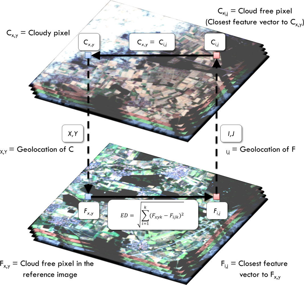
4.4. Image Restoration Algorithm

The basis of the implemented approach is the Closest Spectral Fit (CSF) technique for multi-spectral images proposed by Meng et al.[35]. It requires two input images, a clouded image C and a cloud-free fill image F. Since the spectral information of each pixel beneath a cloud in image C is useless, it is desirable to restore these spectra with the support of the image F. A fundamental assumption is that the co-registration of the images results in a perfect match of the geolocation between the two images. Based on this requirement, the geolocation x, y of every cloudy pixel C_x,y in image C can be recognized in image F. Subsequently, for each of these pixels F_x,y, the spectral distance to all other pixels F_i,j is computed. This distance is derived by the Euclidean Distance (ED), which is given by:

$$\mathit{ED}=\sqrt{\sum _{i=1}^k{\left(F_{\mathit{xyk}}-F_{\mathit{ijk}}\right)}^2}$$

(1)

where k denotes the number of bands, F_x,y,k represents the digital numbers of the reference pixel at the geolocation x, y in the band k, and F_ijk defines the DN of a pixel at the geolocation i, j, which is compared with the DN at x, y in band k. The smaller the evaluated distance between F_x,y and F_i,j, the higher the similarity between those two pixels. Therefore, the ideal value of ED is zero [35]. After the determination of the spectral distance for each pixel in image F, the geolocation i, j of the spectrally most similar pixel is returned. In case of ambiguous occurrence of minimum values of ED, the pixel that is spatially closest to the geolocation x, y is regarded as best choice. The DN of C_x,y is then substituted by the DN of C_i,j for each Band k. The algorithm introduced by Meng et al.[35] is referred to as Closest Spectral Fit (CSF). Since the aim of this study is the test of a potential integration of SAR data as support image F in a cloud filling approach, the term “spectral” seems misleading. Therefore the abovementioned technique is further referred to as Closest Feature Vector (CFV). Figure 4 gives a schematic overview of the functionality of the CFV approach. Based on the CFV, the spectral neighborhood or the spectral similarity respectively is assessed and used as the criterion to identify the most appropriate pixel to fill the information gap produced by a certain cloudy pixel. In the framework of this study, the approach is extended by the very fundamental assumption of spatial correlation. Justified by the first law of geography, it is assumed that “everything is related to everything else, but near things are more related than distant things.” [18]. Therefore the spatial distance of a pixel F_i,j to the pixel F_x,y is considered as a weighting factor by means of the Spatial Euclidean Distance (SD) by:

$$\mathit{SD}=\sqrt{\sum _{i=1}^k{\left(F_x-F_i\right)}^2+{\left(F_y-F_j\right)}^2}$$

(2)

where F_x and F_y are the x- and the y-coordinate of the reference pixel and F_i and F_j are the x- and y-coordinate of the pixel of which distance is the subject of investigation. The distance weight of a certain pixel is implemented by the usage of an Inverse Distance Weighting (IDW) function, which is calculated for every pixel in the image. Hence, pixels proximate to F_x,y carry a larger weight than points in larger spatial distance [14]. IDW is implemented as:

$$\mathit{IDW}=\frac{1}{{\left(\frac{\mathit{SD}}{R}\right)}^{\beta }}$$

(3)

with the spatial resolution R of the image and a calibration factor β, which is responsible for the strength of the decrease of the weight in dependence of the distance. The provision for R is implemented due to two reasons. First the weighting function is supposed to account for the absolute metric distance. Second, in case the absolute metric distance is neglected, SD tends to become zero for remote pixel. Based on the given remarks, the final determination of the most appropriate pixel C_i,j for the removal of a cloudy pixel C_x,y is given by:

$$C_{i,j}=\mathit{CFV}\cdot \mathit{IDW}$$

(4)

In case two or more pixels gained the same weight due to the estimation of their feature vector and their spatial distance, the pixel with the smallest spatial distance is chosen as appropriate fill pixel for C_x,y. We implemented two different approaches to fill cloudy pixels based on the determined CFV. A standard approach, which was used in this study, is based on the assumption that the spectral information of a clouded pixel C_x,y is completely lost for all spectral bands. Therefore the information of all spectral bands k is replaced by the spectral information of the respective spectral band k of the CFV. An alternative approach is useful in case only single bands of a certain pixel are corrupted. In this case only certain bands of this pixel are reconstructed. This scenario applies for the Landsat ETM+ SLC-Off effect, for example.

4.5. Statistical Quality Assessment

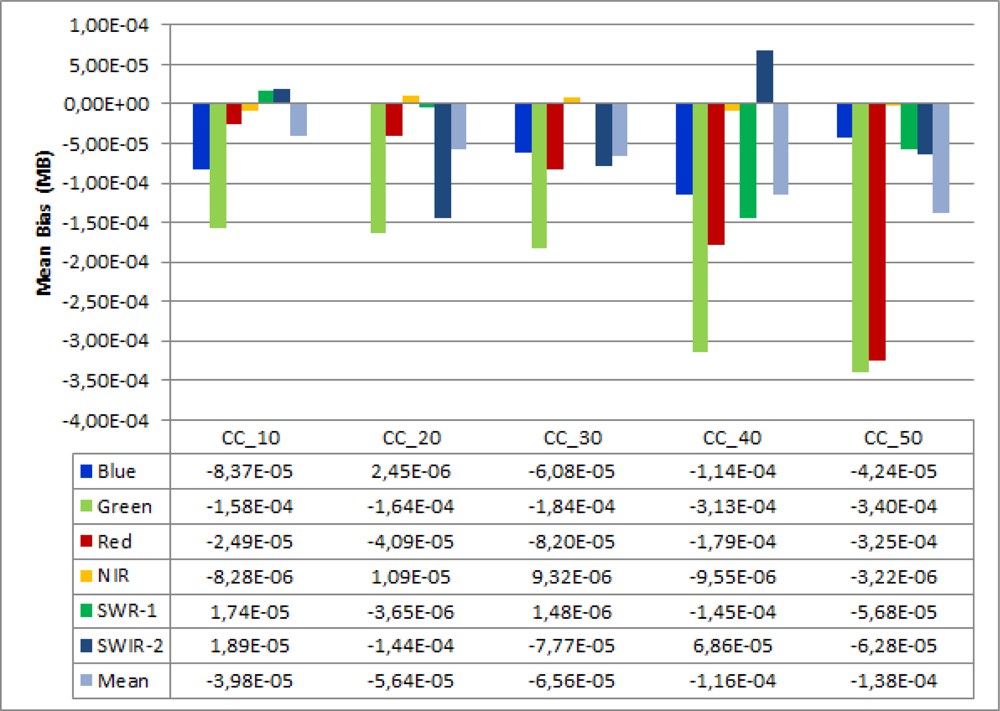
In order to provide a reliable and robust statistical evaluation of the products of the cloud removal, it is mandatory to apply meaningful and effective statistical measures. Thomas and Wald [36] propose a general framework for a quality assessment of a fused image product. Thomas and Wald [37] propose a categorization of statistical distances to measure the quality of a fused image in comparison to a reference. This categorization enables the tackling of every aspect of image comparison. On the other hand, redundancies amongst the measures can be avoided. Since the categorization is developed mainly for image fusion methods for the sake of an enhancement of the spatial resolution, the evaluation framework is slightly adopted in the framework of this study. The selection of the statistical measurements is based upon the recommendations of Thomas and Wald [36], Wald et al.[38] and the findings of Berger et al.[39].

Mean Bias

A measure of the global differences between the original and the filled image is the Mean Bias (MB):

$$\mathit{MB}=\frac{\mu \left(F_k\right)-\mu \left(O_k\right)}{\mu \left(O_k\right)}$$

(5)

where μ(F_k) and μ(O_k) are the mean values of the filled image and the original reference image for the spectral band k respectively. Since this measure illustrates the difference between the two compared images, the ideal value is zero. A positive value of MB indicates a minor spectral preservation. A negative value of MB is an evidence for too many spectral innovations [37].

Loss/Gain of Image Content

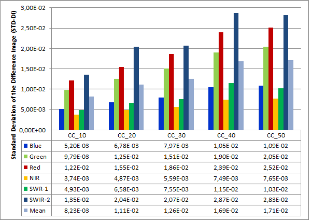
The gain or loss of image content can be quantified by computations of the image differences in terms of their variability. The Difference of Variances (DV) is given by:

$$\mathit{DV}=\frac{{\left(\sigma \left(F_k\right)\right)}^2-{\left(\sigma \left(O_k\right)\right)}^2}{{\left(\sigma \left(O_k\right)\right)}^2}$$

(6)

where σ (F_k) and σ (O_k) are the standard deviations of the filled image and the original image for each spectral band k. A positive value of DV indicates the introduction of artificial image content, since the variance of the filled image will be larger than the variance of the reference image. On the other hand, a negative value indicates a loss of information content. Therefore the ideal value for this measure is zero [38].

Image of Difference

The Standard Deviation of the Difference Images (STD-DI) represents the level of the per-pixel error as a global measure, denoted by:

$$\mathit{STD}-\mathit{DI}=\frac{\sigma \left(F_k-O_k\right)}{\mu \left(O_k\right)}$$

(7)

with the standard deviation σ of the difference between the filled image and the original image, for every band k, divided by the mean of the original image μ(o_k) for the band k. The ideal value of this measure is zero, which indicates perfect similarity of the two images [38].

Structural Similarity

The Correlation Coefficient (CC) is applied to measure the performance in terms of the similarity of small size structures between the reference image and the filled image. It is given by:

$$\mathit{CC}=\frac{{\sum }_{i=1}^n{\sum }_{i=1}^m\left(O_{\mathit{ijk}}-\mu \left(O\right)\right)\cdot \left(F_{\mathit{ijk}}-\mu \left(F\right)\right)}{\sqrt{{\sum }_{i=1}^n{\sum }_{i=1}^m{\left(O_{\mathit{ijk}}-\mu \left(O\right)\right)}^2\cdot {\left(F_{\mathit{ijk}}-\mu \left(F\right)\right)}^2}}$$

(8)

where O_ijk and F_ijk are the elements of the images O and F (i.e., pixels) in Band k for all columns n and all rows m. The means of the filled image and the original image are given by μ(F_k) and μ(O_k). Since this measure expresses the structural similarity of the two images, the ideal value is one [37].

Spectral Fidelity

A measure for the spectral differences between the images is given by the Spectral Angle Mapper (SAM). The angle α is calculated on the k-dimensional vectors of the spectra of a pixel O_ij and F_ij[40]. SAM is defined as:

$$\mathit{SAM}={\text{cos}}^{-}1\left(\frac{\overrightarrow{O_{\mathit{ij}}}\cdot \overrightarrow{F_{\mathit{ij}}}}{\Vert \overrightarrow{O_{\mathit{ij}}}\Vert \cdot \Vert \overrightarrow{F_{\mathit{ij}}}\Vert }\right)$$

(9)

where $\overrightarrow{O_{\mathit{ij}}}$ and $\overrightarrow{F_{\mathit{ij}}}$ are representing the vectors in the k-dimensional multi-spectral feature space for each pixel at the location (i, j). The pixel-wise computation of SAM is averaged for the whole image. A small SAM indicates a high spectral similarity between the filled image and the original image. The ideal value is therefore zero [40–42].

4.6. Design of the Performance Evaluation

4.6.1. Proof of Concept

The first major part towards the evaluation of the potential of SAR data to remove cloud-obscured pixels from multi-spectral imagery is a reliable test of the algorithm performance. Therefore it is mandatory to prove the potential of the techniques to restore information beneath clouds. In this study, an approach is established that contains two steps.

• Cloud removal based on a perfect fill image.
• Cloud removal based on a multispectral image.

A perfect data source in terms of information restoration is the clouded image itself. This seems paradoxical at first glance, since it raises the question of how an image filled by a certain algorithm with itself shall prove the performance of the algorithm. However, instead of replacing the feature vector of a certain pixel with itself, the algorithm will find the spectrally and spatially closest neighbor. The regions beneath the clouds are masked out for the derivation of the CFV. This methodology makes sure that the fill algorithm will find the most similar pixel F_i,j for the pixel F_x,y under investigation. This approach has numerous advantages. First, it enables the investigation of the overall performance potential of the fill algorithm. Will the result be also perfect, considering a perfect data source? Second, the influence of the two components of the fill algorithm (i.e., CFV and IDW) on the fill result can be evaluated in order to define an optimal distance weight (DW). The major shortcoming is the fact that such a perfect data source for cloud removal will hardly exist in the real world, since it assumes the same acquisition date, the same radiometric properties, the same spatial and spectral resolution and exactly the same atmospheric conditions of the fill image F in comparison with the clouded image C. Nevertheless, this theoretical evaluation of the fill algorithm performance is a significant step towards the evaluation of the algorithm performance. In order to estimate the influence of DW as well as the general potential, a number of constellations are established. First, the amount of cloud cover was fixed at 10%. Only the weight DW is varied. Second, DW is fixed and the amount of cloud cover is varied. The distance weight is varied from 0.0 (i.e., distance has no influence) over non-linear values (cf. Figure 5) up to 2.0. In the latter case the weight of the distance changes with the square of the distance. This property is tested due to the fact that DW = 2.0 is the most common setting in spatial interpolation techniques using IDW [14]. The amount of cloud cover was varied from 10% to 50% in order to evaluate the loss of restoration quality due to the limitation of available information.

The second step towards the assessment of the potential of SAR data is the evaluation of the performance potential of the algorithm by means of an additional multi-spectral reference. This is useful in terms of testing the robustness of the fill algorithm with regard to variations in the number of available spectral bands, their specific bandwidth, etc. Therefore, the knowledge about the potential of the fill algorithm to compensate these variations will be a significant advancement. This second step was accomplished within this study with the help of a SPOT 4 scene of the test site. This SPOT image was filled by means of the Landsat scene. A major shortcoming is the fact that the overlapping area between the SPOT 4 and the SAR scenes is very small. Therefore the spatial subset varies for this part of the study. The distance weighting function was configured according to the findings of the performance evaluation by means of the perfect data source, and it was therefore fixed at 0.0. The amount of cloud cover was varied from 10% to 30% following the same premise as in the evaluation with the perfect data source. The findings are documented in Section 5.1.

4.6.2. Experimental Setup of the Multi-Frequency SAR Analysis

As second major part, the capability of SAR data to remove cloud cover from multi-spectral images by means of the given algorithm had to be tested using a huge variety of constellations in order to find the best setup for cloud removal. The tested data constellations are shown in Figure 6. Therefore, the backscatter intensities of the SAR data were included as reference data in the image reconstruction as single frequency information as well as a multi-frequency dataset of X-, C- and L-Band data. To enhance the dimensionality of the SAR information, texture measures were included since texture is supposed to increase the separability of structural features within the images [43]. Hence, a set of co-occurrence texture measures was estimated from the SAR intensity images with a 3 × 3 mowing window and added to the stack of SAR data. The texture measures Contrast, Dissimilarity, Homogeneity, Mean and Variance were derived [43,44].

5. Results

5.1. Results of the Proof of Concept

5.1.1. Sensitivity to the Distance Weighting

The variation of the distance weight shows sensitivity of the removal result to this parameter. Although the variation is very small, there is a significant trend. The increase of DW entails a loss of image restoration quality. The filled images tend to be slightly negatively biased, which indicates artificial spectral innovations. The negative values of the DV indicate a loss of image content since the variance of the filled image is lower than the variance of the original image. In addition, the STD-DI points to a loss of similarity between the original image and the filled image by increasing DW. Although the Correlation Coefficient varies only at the third digital place, the decrease with an increase of DW is obvious. SAM as a measure for the spectral fidelity of the image also behaves inversely proportional to the variation of DW. All evaluated statistical measures are varying in very small intervals from their ideal value, which could be regarded as an indicator of a very high performance of the algorithm despite the variation of the inverse distance weighting function. On the other hand, this strong similarity of the statistical cloud removal results provides the opportunity to evaluate the sufficiency of the statistical measures to capture the findings of the cloud removal process. Therefore it is expedient to include a visual comparison of the removal results into the assessment (Figure 5).

5.1.2. Sensitivity to the Amount of Cloud Cover

As a next step, the loss of quality in the filled images was examined with a changing amount of cloud cover (CC) (cf. Figure 7). The percentage of cloud cover was varied from 10% to 50% to evaluate the stability of the restoration result depending on the amount of available information for the fill algorithm. The DN of all filled images slightly tend to indicate artificial spectral innovation since they are negatively biased (Figure 8). The negative values of the DV indicate a loss of image content (Figure 9). The similarity between the original image and the filled image decreases with the increase of the percentage of cloud cover, indicated by an increase of the STD-DI (Figure 10). The Correlation Coefficient has only a small deviation but also shows a decreasing trend with increasing cloud cover (Figure 11). Also SAM only slightly increases but follows the major trend of all statistical measures (

Table 3. Spectral Angle Mapper.

	CC 10%	CC 20%	CC 30%	CC 40%	CC 50%
SAM	0.4535	0.4539	0.4545	0.4551	0.4567

). The magnitude of the deviations compared with the particular optimum value of the statistical measure is very small, which indicates a very good image restoration result. The fill algorithm is very stable in terms of the number of available pixels for the derivation of the CFV.

Figure 7 gives a visual overview of the results for a small image subset. The changes are very small and the restoration of the original DN evinces a very high performance. The findings of the image restoration by means of a perfect data source can be outlined as follows:

• The integration of an inverse distance weighting function causes a loss of image restoration quality. IDW is therefore neglected in further image restoration steps.
• The cloud removal algorithm is capable to compensate for a high percentage of cloud cover, provided that the quality of the data source is sufficient.
• The set of statistical measures is not sufficient to completely describe the image quality. Therefore a visual comparison is mandatory.

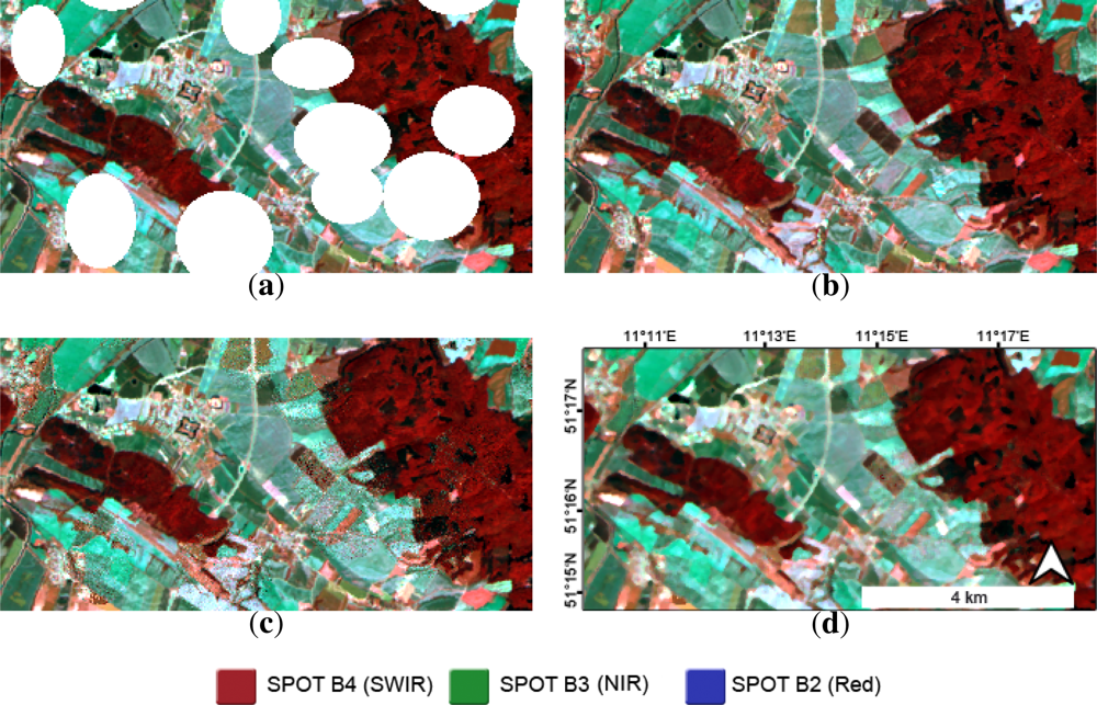
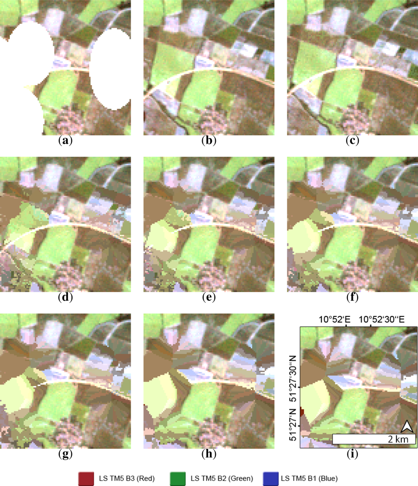
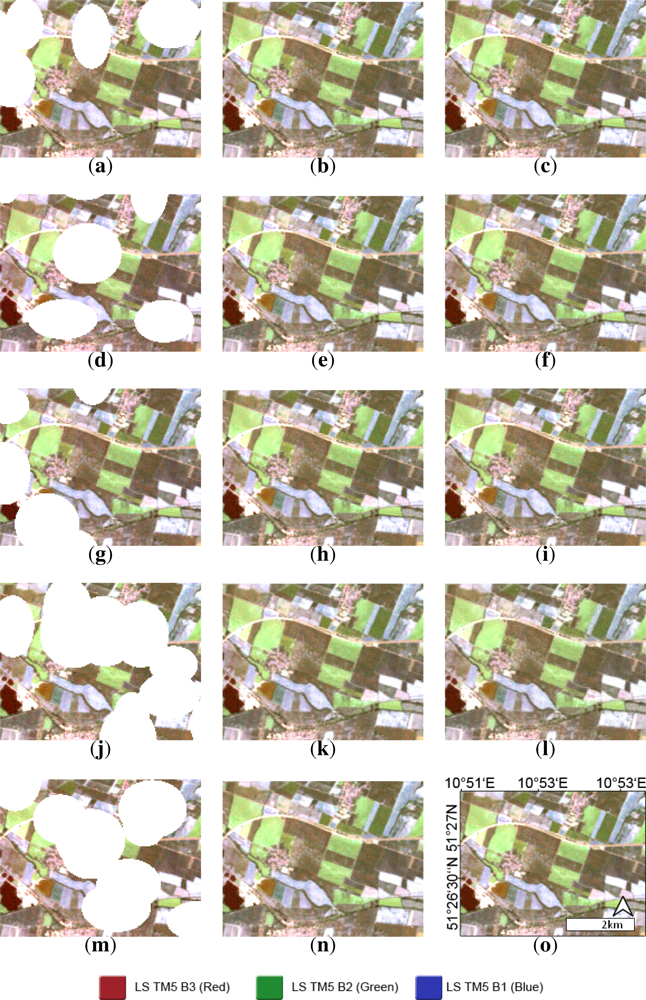
5.1.3. Cloud Removal by Means of a Multi-Spectral Reference Image

On the way towards the rating of the potential of SAR data to fill images obscured by clouds, the image restoration by means of a multi-spectral data source is mandatory to serve as a reference value of expectancy. Figure 12 shows the results of the reconstruction of missing values within the SPOT 4 scene. Figure 12(b,c) compares the original with the filled image. Furthermore, Figure 12(d) displays a visual example of the enhanced image quality due to further spatial averaging (3 × 3 Median filter). The findings of the image restoration by means of a multi-spectral image can be outlined as follows:

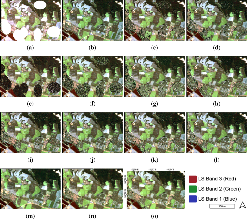
• The integration of a real existing dataset in the algorithm enables the removal of cloud cover from multi-spectral images, resulting in a meaningful image content of the restored image.
• The visual appearance of the restored areas is affected by clutter noise. The origin of this noise needs further investigation. It appears to be helpful to compensate for this effect by means of spatial averaging.

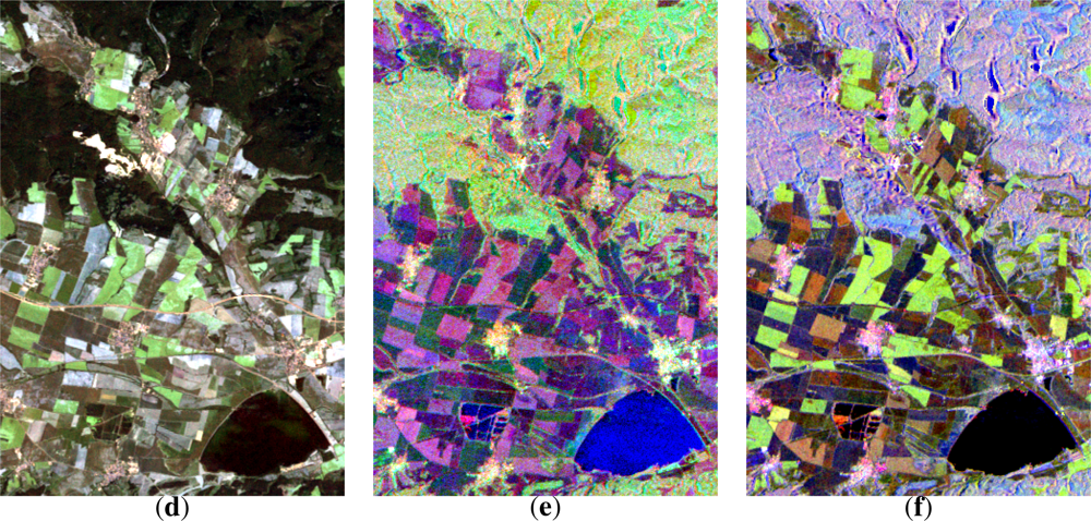
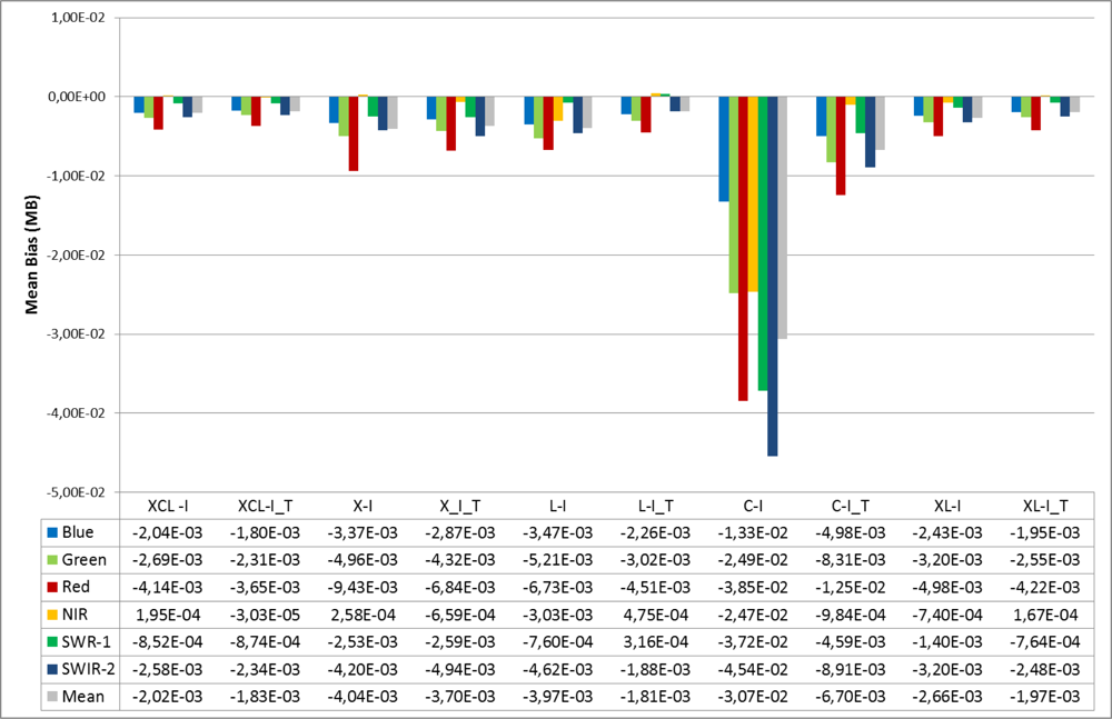
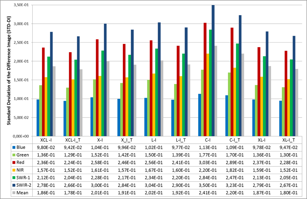
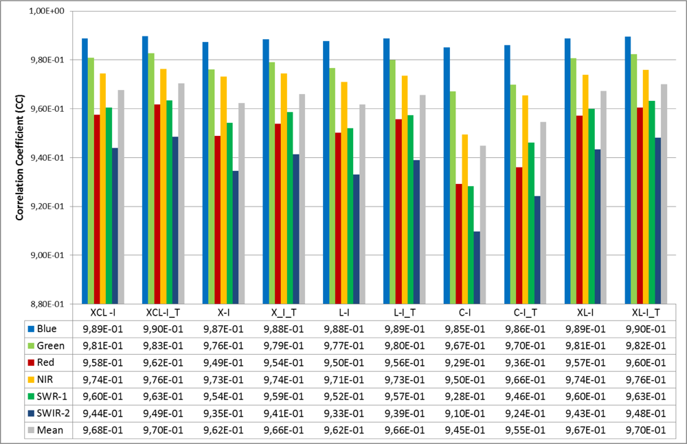
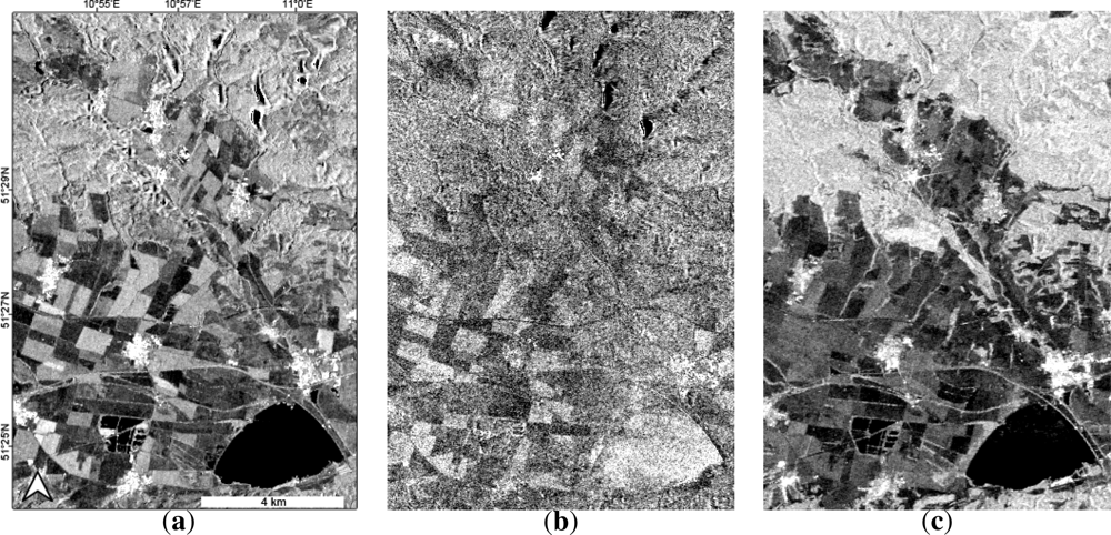
5.2. Findings of the Multi-Frequency SAR Analysis

Since the integration of multi-frequency SAR data into the image reconstruction process is the main part of the proposed workflow, the statistical evaluation of the results is presented in detail. The mentioned statistics are calculated for the entire image, not only the cloud masked areas. The results of the mean preservation of the image content by using the MB indicate a spill-over of spectral innovations since almost all reconstructed image bands in all frequency combinations are negatively biased (Figure 13). The weakest performance is achieved by C-Band, which is outperformed by all other combinations by orders of magnitudes. The visible bands, especially the Red band, are most biased, while the infrared bands are in general less biased. The results tend to a loss of image content since the majority of the reconstructed bands have a negative DV (Figure 14). Only NIR and SWIR-1 tend to be subject to the introduction of artificial image content for the most of the frequency combinations. The level of the per-pixel error is denoted by the STD-DI. For the analysis of several frequency combinations, this measure shows no significant differences. The highest deviations from the ideal value are observed for C-Band Intensity and C-Band Intensity + Texture (Figure 15). The structural similarity of the filled and the reference image, which is expressed by the Correlation Coefficient, shows very high values for all bands in all frequency combinations (Figure 16). Only C-Band Intensity features a slightly weaker performance in terms of structural similarity. The spectral fidelity of the filled images is evaluated by means of SAM. The smallest spectral differences are achieved by the combination of XL-Band Intensity + Texture as well as XCL-Band Intensity + Texture (

Table 4. Spectral angle mapper.

	XCL-I	XCL-I_T	X-I	X-I_T	L-I	L-I_T	C-I	C-I_T	XL-I	XL-I_T
SAM	0.496	0.495	0.497	0.497	0.499	0.497	0.506	0.501	0.496	0.495

). The lowest spectral fidelity is achieved with C-Band Intensity and C-Band Intensity + Texture.

Several findings result from these statistical evaluations of the fill quality. In every category the frequency combinations C-Band Intensity and C-Band Intensity + Texture appear to have the lowest performance. In order to increase the certainty of the performance of the several frequency combinations, the values for each statistical measurement at each band were ranked according to their deviation from the particular optimal value. The result is presented in

Table 5. Ranking of the frequency combinations for the full image. The color ranges from red (worst case) to green (best case) indicate the statistical performance of the frequency band combinations.

	X-I	XI_T	C-I	C-I_T	L-I	L-I_T	XL-I	XL-I_T	XCL-I	XCL-I_T
MB_Red	7	6	10	9	8	4	5	2	3	1
MB_Green	7	6	10	9	8	4	5	2	3	1
MB_Blue	8	7	10	9	6	4	5	3	2	1
MB_NIR	4	6	10	8	9	5	7	2	3	1
MB_SWIR-1	7	8	10	9	2	1	6	3	4	5
MB_SWIR-2	6	8	10	9	7	1	5	3	4	2
MB_Mean	8	6	10	9	7	1	5	3	4	2
DV_Red	8	6	10	9	5	4	7	2	3	1
DV_Green	8	6	10	9	7	4	5	3	1	2
DV_Blue	9	7	10	8	1	5	4	6	2	3
DV_NIR	8	7	10	6	9	1	2	3	5	4
DV_SWIR-1	2	6	10	9	8	7	1	4	5	3
DV_SWIR-2	7	6	10	9	8	1	3	5	2	4
DV_Mean	8	6	10	9	7	4	5	3	1	2
STD-DI_Red	8	6	10	9	7	3	4	2	5	1
STD-DI_Green	8	6	10	9	7	5	4	2	3	1
STD-DI_Blue	8	6	10	9	7	5	4	2	3	1
STD-DI_NIR	7	3	10	9	8	6	5	2	4	1
STD-DI_SWIR-1	7	5	10	9	8	6	4	2	3	1
STD-DI_SWIR-2	7	5	10	9	8	6	4	2	3	1
STD-DI_Mean	7	5	10	9	8	6	4	2	3	1
CC_Red	8	6	10	9	7	3	4	2	5	1
CC_Green	8	6	10	9	7	5	4	2	3	1
CC_Blue	8	6	10	9	7	5	4	2	3	1
CC_NIR	7	3	10	9	8	6	5	2	4	1
CC_SWIR-1	7	5	10	9	8	6	4	2	3	1
CC_SWIR-2	7	5	10	9	8	6	4	2	3	1
CC_Mean	7	5	10	9	8	6	4	2	3	1
SAM	7	5	10	9	8	6	4	2	3	1
Mean	7,17241	5,7931	10	8,82759	7,10345	4,34483	4,37931	2,55172	3,2069	1,62069
Final Rank	8	6	10	9	7	4	5	2	3	1

. The values rank from 10 (largest deviation) to 1 (smallest deviation). The best mean ranking of all values over all image bands is used to determine the statistically best frequency constellation to restore data gaps due to cloud cover. Based on the results of this ranking, the combination of multiple frequencies is clearly preferable compared with a mono-frequency data basis. Furthermore, the inclusion of the mentioned texture measures increases the performance of the cloud removal algorithm in every case. The findings of the image restoration of the full image by means of multi-frequency SAR data can be outlined as follows (cf. Figure 17).

• The combination of more than one SAR frequency increases the restoration quality.
• The restoration with inclusion of the derived texture measures outperforms the frequency combinations without texture.
• Concerning mono-frequency SAR data, L-Band is most suitable for image restoration. For multi-frequency SAR data, the frequency combination XCL features the best statistical budget.
• Due to the poor data quality of the used ERS image, C-Band data is excluded from any interpretation of the study results.

To conclude, Figure 18 shows the reconstruction result for the test area.

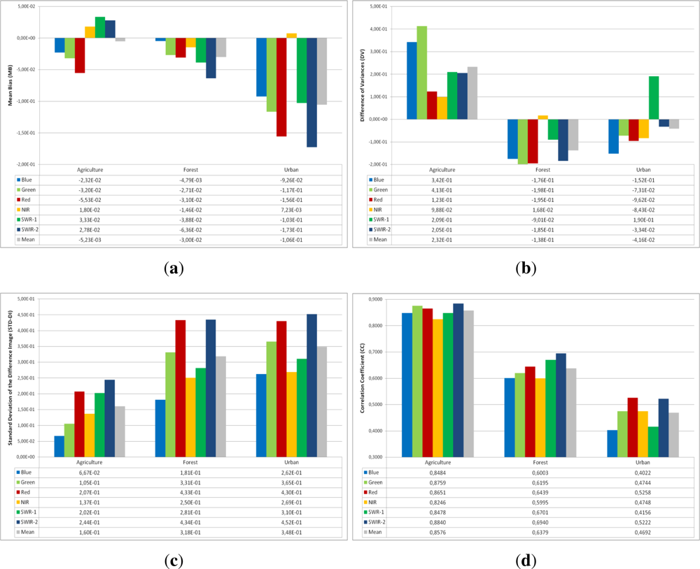
5.3. Sensitivity to Land Cover Types

As a last step of the assessment procedure, the reconstruction quality was evaluated with focus on certain land cover classes. The analyzed categories included agriculture, forest and urban areas. The statistical evaluation was examined for all frequency combinations except C-Band Intensity and C-Band Intensity + Texture, which were skipped according to the findings of the investigation of the full image. Since the statistics of all frequency combinations are similar, only the frequency combination XL-Band Intensity + Texture is presented here. Urban areas are most biased (Figure 19(a)). The agriculture and forest areas are biased in approximately the same order of magnitude. The mainly negative values for MB indicate the occurrence of artificial spectral innovations. The DV is negative in general (Figure 19(b)). Therefore, the image content of the restored image can be regarded as reduced in comparison with the original. Again, urban areas highlight the weakest statistical performance in terms of the preservation of image content. Figure 19(c) shows the STD-DI. This measurement indicates that agricultural areas are reconstructed well with respect to the original image. The forest and urban areas show a similarity to the original image in the same order of magnitude. Also the structural similarity, indicated by the Correlation Coefficient, is highest for the agriculture areas, medium for the forest areas and weakest for urban areas (Figure 19(d)). In terms of the spectral fidelity, the same trend is observable. SAM is closest to the ideal value 0 for agriculture and features the highest deviations in urban areas (

Table 6. Spectral angle mapper.

	Agriculture	Forest	Urban
SAM	0.0917	0.1100	0.1558

).

The findings of the land cover specific examination can be outlined as follows:

• Urban areas are restored with the lowest quality. The forest and agriculture areas are restored with a similar quality, but with certain differences depending on the facet of image restoration that is focused on.
• The statistics can be regarded as verification of the theoretical anticipations that more homogeneous land cover classes achieve better restorations results than heterogeneous categories.

6. Discussion

6.1. Methodology

The depicted framework of this study, comprising cloud simulation, image reconstruction and statistical evaluation, was designed as basic research tool for (1) the evaluation of the performance of the Closest Feature Vector (CFV) technique, and (2) the potential of space-borne SAR data to fill data gaps in multi-spectral imagery. The cloud simulation is a mandatory part since it facilitates the comparison of the original image with the reconstructed image based on statistics. The application to a real case, i.e., integrating the image reconstruction together with cloud detection in an actually clouded image, can be considered as a subsequent research topic. In this study, this “real case scenario” was not considered, since the focus of the conducted work was on analyzing the capability of SAR data together with CFV to reconstruct data gaps. Therefore, the artificial introduction of missing information was mandatory.

The statistical evaluation protocol covered every aspect of image quality according to Thomas and Wald [37]. This study was focused on the assessment of the overall feasibility of the integration of SAR data as a reference for cloud removal. Therefore, the global image quality was assessed by comparing every pixel of the original image to every pixel of the reconstructed image. Using this approach, conclusions on the overall image quality for classification, parameter retrieval, etc., can be drawn. Therefore all statistics shown in this study were derived straightforwardly by this method. As an alternative, a detailed reconstruction quality can be assessed by evaluating the statistical protocol only for filled areas. This approach allows for an enhanced understanding of error sources in the fill algorithm. This statistical evaluation can be considered as useful tool for further development of the fill algorithm and for the analysis of the nature of clutter and noise effects. Nevertheless, this detailed error analysis was beyond the focus of this study.

The used reconstruction approach depicts a special form of the concept of image fusion. By definition “image fusion is the combination of two or more different images to form a new image by using a certain algorithm” [45]. The proposed approach does not denote the fusion of the pixel DN values per se; the algorithm rather makes use of a derivation of geolocation values. This is a major advantage in comparison with any substitution technique since the reconstructed DNs are completely retrieved from the very image that is supposed to be filled. Therefore, based on the assumption of homogenous atmospheric conditions within every image, atmospheric and radiometric corrections between the images are not necessary when following the proposed approach. Nevertheless, certain requirements are made on the data basis. The coregistration of optical and SAR data has to be as accurate as possible to avoid the mismatch of pixels. This is the major prerequisite for the successful application of the algorithm. It is also very important to correct for the differing viewing geometries of optical and SAR data. Topographic normalization of the Radar images is necessary to avoid artifacts from SAR shadow, Layover and Foreshortening effects. The restoration accuracy also depends on the time gaps between the clouded image and the fill image. In general, it is understood that the shorter the time span between the acquisition of the two images, the better the reconstruction quality, since the land cover was not changing too much. In this study, the time span between the optical and SAR data was not bigger than three days, which can be considered as an optimal case. Furthermore, the reconstruction quality highly depends on the underlying land cover class and their affection to seasonal changes. For highly variable classes, e.g., agriculture, the reconstruction based on data from a similar season should be preferred.

The algorithm is capable to incorporate very diverse data sources. This was demonstrated by the integration of Landsat TM 5, SPOT 4, ERS, ALOS PalSAR and TerraSAR-X data. Based on these results, the CFV technique, which can be regarded as a modification of the Closest Spectral Fit technique proposed by Meng et al.[35], is found to fulfill the requirements of a generic and sensor independent approach that is simple and efficient.

6.2. Is Cloud Removal Feasible with SAR Data?

The major hypothesis within this study is the similarity of physically based relations between the reflectance in the VIS/NIR part and the microwave part of the EM spectrum. As already demonstrated by means of Figure 1, VIS/NIR reflectance and SAR backscatter are closely related. Nevertheless, the information is not completely similar. One drawback of the proposed method is the fact that multi-frequency information is needed to represent the information content of the multi-spectral imagery via SAR data. Further investigations on the similarity of single as well as multiple frequency bands with multi-spectral imagery are necessary to draw final conclusions. The performance of single frequency SAR bands for cloud removal is highly variable. Justified by the data quality, the results of the C-Band data should be excluded from any interpretation in this specific study. For the frequencies X- and L-Band it is not possible to draw uniform conclusions. The statistical quality is very variable regarding the different Landsat image bands. The rankings (cf. Table 5) indicate that L-Band performs better than X-Band in terms of the statistical evaluation protocol. The visual comparison depicts a better capability of edge preservation in agricultural areas at X-Band, but a better restoration of DNs in forests at L-Band. Hence, it is recommended to carry out a more detailed quality evaluation with various land cover types before drawing final conclusions.

SAR speckle may be a source of clutter in the restored images. The influence of speckle is reduced significantly due to the partially very strong multi-looking of the data. Nevertheless, the influence of speckle is still not negligible. This clearly indicates that filtering is a suitable approach to increase the image reconstruction quality. In this study, spatial averaging was carried out by simple median filtering using a 3 × 3 pixel kernel size. A further examination of averaging techniques was beyond the focus of this study. According to the study results, a major improvement of the image restoration results can be expected by a suitable definition of spatial averaging algorithms. For this reason, the image fusion should be carried out on a higher level. Feature level fusion (cf.[45]) prepends the extraction of non-overlapping adjacent homogeneous image objects before the virtual image restoration. The extraction of image objects enables the reduction of the influence of speckle [46]. Furthermore, an object oriented approach would allow for the compensation of spatial scale dependencies due to divergent spatial resolutions of the input data.

Multi-frequency SAR data outperform single frequency fill images in terms of statistical quality. This is indicating that the introduction of several wavelengths is stabilizing the capability to relate SAR backscatter intensity to optical/infrared reflectance. On the other hand, it has to be kept in mind that an increase of frequency bands, and therefore texture layers, is supposed to increase the quality by definition. As the number of layers contributing to the derivation of the Closest Feature Vector of a certain pixel increases, the agreement is more reliable. Therefore, it is in dispute if the increasing statistical quality is based on the inclusion of multiple SAR frequencies or simply the result of the inclusion of a higher number of image layers.

7. Conclusions and Outlook

This study focuses on the problem of cloud cover in multi-spectral satellite data. The presented approach combines the Closest Spectral Fit (CSF) algorithm proposed by Meng et al.[35] with the synergistic application of multi-spectral satellite images and multi-frequency Synthetic Aperture Radar (SAR) data. The image restoration algorithm overcomes several disadvantages of other methods. As the algorithm replaces missing digital numbers (DNs) with information from the same image, a radiometric calibration becomes obsolete. Furthermore, the approach is independent of sensor specifications, land cover types or seasonal dynamics. The analyses are embedded in a statistically reliable framework, which is capable to investigate the image reconstruction quality based on objective measures. The applied methodology includes a three stage approach comprising an examination of the plausibility of the CSF method, the reconstruction of a multi-spectral SPOT image by means of a Landsat image, as well as the reconstruction of cloud contaminated areas in a Landsat image with the aid of multi-frequency SAR data. The results indicate the potential of mono-temporal SAR data to overcome data gaps in multi-spectral images under certain restrictions. The outcomes evidently show that a synergistic usage of the complementary nature of multi-spectral and SAR satellite images can help to overcome limitations in data availability and quality.

An urgent need for future work resulting from this study is the implementation of the algorithm and experimental setup in a greater framework. Only in case of further improvements can this approach make its way towards an operational approach. Based on the study findings and the implications discussed, three major aspects of possible future research are summarized here. The integration of object based approaches as an avenue to adaptive spatial averaging implies a great potential to increase the homogeneity and reliability of the image restoration results. The extraction of small, non-overlapping homogenous objects may significantly enhance the usability of the data, especially in the framework of land cover classifications. According to the results of the study, the integration of additional information increases the agreement certainty and therefore the image reconstruction quality. At the moment, the examination of interferometric coherence data would violate the rule of short temporal baselines. However, in the course of the ESA Living Planet program, the C-Band SAR Satellite constellation Sentinel 1A and 1B will enable the derivation of coherence data with a revisit cycle of 6 days [47,48]. This temporal baseline would enable the integration of this type of information into the image restoration process. Furthermore, the potential of full-polarimetric SAR systems (e.g., TerraSAR-X/TanDEM-X, ALOS PalSAR) is worth exploring.

In addition, the integration of multi-spectral data in order to remove cloud cover from different multi-spectral images should be the subject of further investigation. Sensors with a high temporal resolution (e.g., MODIS [49]) have the inherent potential to overcome the drawback of significant land cover changes between the image acquisitions. Furthermore, this study indicated that the image reconstruction quality in case of a multi-spectral fill image is very high (cf. Section 5.1.3).

An essential step towards the evaluation of the operational practicability of the presented approach is an extensive investigation of the restoration sufficiency of certain land cover types. For a reliable knowledge of the expectable reconstruction quality of a certain land cover class, the analysis must be applied to distinct agricultural classes, biotope habitats, different forest types, urban areas, etc.

Furthermore, the application of the CFV technique can be extended to several scientific issues within the field of remote sensing. Since cloud cover can be regarded as areas of unavailable data, also other cases of missing data can be examined. Similar technologies are applied for the correction of the scan-line corrector (SLC) failure in Landsat 7 ETM + data (e.g., [50]). Another possible path of image reconstruction could be the estimation of missing backscatter intensity values in SAR images caused by geometric distortions (i.e., Layover, Foreshortening and Radar shadow) based on additional optical images.

References

1. Rees, W.G. Physical Principles of Remote Sensing, 2 ed.; Cambridge University Press: Cambridge, UK, 2001; p. 343. [Google Scholar]
2. Schowengerdt, R.A. Remote Sensing: Models and Methods for Image Processing, 3 ed.; Elsevier: San Diego, CA, USA, 2007; p. 558. [Google Scholar]
3. Cihlar, J.; Howarth, J. Detection and removal of cloud contamination from AVHRR images. IEEE Trans. Geosci Remote Sens 1994, 32, 583–589. [Google Scholar]
4. Helmer, E.H.; Ruefenacht, B. Cloud-free satellite image mosaics with regression trees and histogram matching. Photogramm. Eng. Remote Sensing 2005, 71, 1079–1089. [Google Scholar]
5. Roerink, J.G.; Menenti, M.; Verhoef, W. Reconstructing cloudfree NDVI composites using Fourier analysis of time series. Int. J. Remote Sens 2000, 21, 1911–1917. [Google Scholar]
6. Sahoo, T.; Patnaik, S. Cloud Removal from Satellite Images Using Auto Associative Neural Network and Stationary Wevlet Transform. Proceedings of First International Conference on Emerging Trends in Engineering and Technology, Nagpur, India, 16–18 July 2008; pp. 100–105.
7. Wang, B.; Ono, A.; Muramatsu, K.; Fuhiwara, N. Automated detection and removal of clouds and their shadows from landsat TM images. IEICE Trans. Inf. Syst. 1999, E82-D, 453–460. [Google Scholar]
8. Lu, D. Detection and substitution of clouds/hazes and their cast shadows on IKONOS images. Int. J. Remote Sens 2007, 28, 4027–4035. [Google Scholar]
9. Martinuzzi, S.; Gould, W.A.; González, O.M.R. Creating Cloud-Free Landsat ETM + Data Sets in Tropical Landscapes: Cloud and Cloud-Shadow Removal; Technical Report; Pacific Northwest Research Statio, US Department of Agriculture-Forest Service: Portland, OR, USA, 2007. [Google Scholar]
10. Song, C.; Woodcock, C.E.; Seto, K.C.; Lenney, M.P.; Macomber, S.A. Classification and change detection using landsat TM data: When and how to correct atmospheric effects? Remote Sen. Environ 2001, 75, 230–244. [Google Scholar]
11. Song, M.; Civco, D.L. A Knowledge-Based Approach for Reducing Cloud and Shadow. Proceedings of ASPRS-ACSM Annual Conference and FIG XXII Congress, Washington, DC, USA, 22–26 April 2002; pp. 1–7.
12. Ren, R.; Guo, S.; Gu, L.; Wang, H. Automatic Thick Cloud Removal for MODIS Remote Sensing Imagery. Proceedings of 2009 IEEE International Conference on Information Engineering and Computer Science, Wuhan, China, 19–20 December 2009; pp. 1–4.
13. Tseng, D.; Tseng, H.; Chien, C. Automatic cloud removal from multi-temporal SPOT images. Appl. Math. Comput 2008, 205, 584–600. [Google Scholar]
14. Webster, R.; Oliver, M.A. Geostatistics for Environmental Scientists, 2nd ed.; Wiley: West Sussex, UK, 2007; p. 315. [Google Scholar]
15. Wen, J.; Su, Z.; Ma, Y. Reconstruction of a cloud-free vegetation index time series for the tibetan plateau. Mt. Res. Dev 2004, 24, 348–353. [Google Scholar]
16. Jupp, D.; Strahler, A.H.; Woodcock, C. Autocorrelation and regularization in digital images. I. Basic theory. IEEE Trans. Geosci. Remote Sens 1988, 26, 463–473. [Google Scholar]
17. Lark, R.M. Geostatistical description of texture on an aerial photograph for discriminating classes of land cover. Int. J. Remote Sens 1996, 17, 2115–2133. [Google Scholar]
18. Tobler, W.R. A computer movie simulating urban growth in the detroit region. Econ. Geogr 1970, 46, 234–240. [Google Scholar]
19. Zhang, C.; Li, W.; Travis, D.J. Restoration of clouded pixels in multispectral remotely sensed imagery with cokriging. Int. J. Remote Sens 2009, 30, 2173–2195. [Google Scholar]
20. Melgani, F. Contextual reconstruction of cloud-contaminated multitemporal multispectral images. IEEE Trans. Geosci. Remote Sens 2006, 44, 442–455. [Google Scholar]
21. Solberg, A.H.S.; Jain, A.K.; Taxt, T. Multisource classification of remotely sensed data: Fusion of Landsat TM and SAR images. IEEE Trans. Geosci. Remote Sens 1994, 32, 768–778. [Google Scholar]
22. Hoan, N.T.; Tateishi, R. Cloud removal of optical image using SAR data for ALOS application. Int. Arch. Photogr. Remote Sens. Spat. Inf. Sci 2008, 37, 379–384. [Google Scholar]
23. Rossow, W.B. Measuring cloud properties from space: A review. J. Clim 1989, 2, 201–213. [Google Scholar]
24. Rodts, S.M.A.; Duynkerke, P.G.; Jonker, H.J.J. Size distributions and dynamical properties of shallow cumulus clouds from aircraft observations and satellite data. J. Atmos. Sci 2003, 60, 1895–1912. [Google Scholar]
25. Gardner, G.Y. Visual Simulation of Clouds. Proceedings of the 12th Annual Conference on Computer Graphics and Interactive Techniques (IGGRAPH ’85), San Francisco, CA, USA, 22–26 July 1985; 19, pp. 297–303.
26. Machado, L.A.T.; Rossow, W.B. Structural characteristics and radiative properties of tropical cloud clusters. Mon. Wea. Rev 1993, 121, 3234–3260. [Google Scholar]
27. Tompkins, A.M. The Parametrization of Cloud Cover; Technical Memorandum, Moist Processes Lecture Note Series; European Centre for Medium-Range Weather Forecasts (ECMWF): Shinfield Park, Reading, England, 2005. [Google Scholar]
28. O’Brien, D.M. Size distributions of clouds in real time from satellite imagery. Int. J. Remote Sens 1987, 8, 817–837. [Google Scholar]
29. Plank, V.G. The size distribution of cumulus clouds in representative Florida populations. J. Appl. Meteorol 1969, 8, 46–67. [Google Scholar]
30. Joseph, J.H.; Cahalan, R.F. Nearest neighbor spacing of fair weather cumulus cluds. J. Appl. Meteorol 1990, 29, 793–805. [Google Scholar]
31. Lee, J.; Chou, J.; Weger, R.C.; Welch, R.M. Clustering, randomness, and regularity in cloud fields. 4. Stratocumulus cloud fileds. J. Geophys. Res 1994, 99, 14461–14480. [Google Scholar]
32. Sengupta, S.K.; Welch, R.M.; Navar, M.S.; Berendes, T.A.; Chen, D.W. Cumulus cloud field morphology ans spatial patterns derived from high spatial resolution landsat imagery. J. Appl. Meteorol 1990, 29, 1245–1267. [Google Scholar]
33. Clark, P.J.; Evans, C.F. Distance to nearest neighbor as a measure of spatial relationships in populations. Ecology 1954, 35, 445–453. [Google Scholar]
34. Pretzsch, H. Analysis and modeling of spatial stand structures. Methodological considerations based on mixed beech-larch stands in Lower Saxony. For. Ecol. Manag 1997, 97, 237–253. [Google Scholar]
35. Meng, Q.; Borders, B.E.; Cieszewski, C.J.; Madden, M. Closest spectral fit for removing clouds and cloud shadows. Photogramm. Eng. Remote Sensing 2009, 75, 569–576. [Google Scholar]
36. Thomas, C.; Wald, L. Assessment of the Quality of Fused Products. Proceedings of 24th EARSeL Symposium, Dubrovnik, Croatia, 25–27 May 2004; pp. 317–325.
37. Thomas, C.; Wald, L. Comparing Distances for Quality Assessment of Fused Images. Proceedings of 26th EARSeL Symposium, Varsovie, Poland, 29 May–02 June 2006; Bochenek, Z., Ed.; 2006; pp. 101–111. [Google Scholar]
38. Wald, L.; Ranchin, T.; Mangolini, M. Fusion of satellite images of different spatial resolutions: Assessing the quality of resulting images. Photogramm. Eng. Remote Sensing 1997, 63, 691–699. [Google Scholar]
39. Berger, C.; Hese, S.; Schmullius, C. Fusion of High Resolution SAR Data and Multispectral Imagery at Pixel Level—A Comparison. Proceedings of 2nd Joint EARSeL Special Interest Groups Workshop, Ghent, Belgium, 22–24 September 2010; pp. 245–268.
40. Kruse, F.A.; Lefkoff, A.B.; Boardman, J.W.; Heidebrecht, K.B.; Shapiro, A.T.; Barloon, P.J.; Gotz, A.F.H. The Spectral Image Processing System (SIPS)—Interactive visualization ans analysis of imaging spctrometer data. Remote Sens. Environ 1993, 44, 145–163. [Google Scholar]
41. Berger, C. Fusion of High Resolution SAR Data and Multispectral Imagery at Pixel Level—A Comprehensive Evaluation. 2010. [Google Scholar]
42. Chibani, Y. Additive integration of SAR features into multispectral SPOT images by means of the à trous wavelet decomposition. ISPRS J. Photogramm 2006, 60, 306–314. [Google Scholar]
43. Haralick, R.M.; Shanmugam, K.; Dinstein, I. Textural features for image classification. IEEE Trans. Syst. Man Cybern 1973, 3, 610–621. [Google Scholar]
44. Hall-Beyer, M. GLCM Texture: A Tutorial. In National Council on Geographic Information and Analysis Remote Sensing Core Curriculum; University of Calgary: Calgary, AB, Canada, 2000. [Google Scholar]
45. Pohl, C.; Van Genderen, J.L. Multisensor image fusion in remote sensing: Concepts, methods and applications. Int. J. Remote Sens 1998, 19, 823–854. [Google Scholar]
46. Thiel, C.; Drezet, P.; Weise, C.; Quegan, S.; Schmullius, C. Radar remote sensing for the delineation of forest cover maps and the detection of deforestation. Forestry 2006, 79, 589–597. [Google Scholar]
47. Attema, E.; Bargellini, P.; Edwards, P.; Levrini, G.; Lokas, S.; Moeller, L.; Rosich-Tell, B.; Secchi, P.; Torres, R.; Davidson, M.; et al. Sentinel-1. The radar mission for GMES operational land and sea services. ESA Bull 2007, 131, 10–17. [Google Scholar]
48. Snoeij, P.; Attema, E.; Torres, R.; Levrini, G.; Croci, R.; L’Abbate, M.; Pietropaolo, A.; Rostan, F.; Huchler, M. Sentinel 1—The Future GMES C-Band SAR Mission. Proceedings of the 6th European Radar Conference, Rome, Italy, 30 September–2 October 2009; pp. 21–24.
49. Justice, C.O.; Vermote, E.; Townshend, J.R.G.; Defries, R.; Roy, D.P.; Hall, D.K.; Salomonson, V.V.; Privette, J.L.; Riggs, G.; Strahler, A.; et al. The Moderate Resolution Imaging Spectroradiometer (MODIS): Land remote sensing for global change research. IEEE Trans. Geosci. Remote Sens 1998, 36, 1228–1249. [Google Scholar]
50. Chen, J.; Zhu, X.; Vogelmann, J.E.; Gao, F.; Jin, S. A simple and effective method for filling gaps in Landsat ETM+ SLC-off images. Remote Sens. Environ 2011, 115, 1053–1064. [Google Scholar]
Figure 1. Comparison of SAR backscatter intensities, a Landsat multi-spectral image and SAR color composites. (a) X-HH; (b) C-VV; (c) L-HH; (d) TM5 B3|B2|B1; (e) X-HH|L-HH|C-VV; (f) X-HH|X-HV|L-HH.
Remotesensing 05 02973f1aRemotesensing 05 02973f1b
Figure 2. Workflow of the study.
Remotesensing 05 02973f2
Figure 3. The testing area “Goldene Aue” in Germany.
Remotesensing 05 02973f3
Figure 4. The Closest Feature Vector (CFV) is determined for each cloudy pixel Cx,y by returning its geolocation to a cloud-free fill image. The Euclidean Distance (ED) for each image band k is calculated for the Pixel Fx,y. The Pixel Fi,j representing the most similar properties to Fx,y is referred to as CFV. The geolocation of this CFV is returned in order to obtain the DNs of the Pixel Ci,j. These DNs are used to substitute the cloudy pixel Cx,y. (after Meng et al.[35]).
Remotesensing 05 02973f4
Figure 5. Visual comparison of the original image in comparison with a filled image by means of a perfect data source (i.e., the image itself) as a function of the Inverse Distance Weighting. (a) Clouded Image; (b) Original Image; (c) IDW = 0.0; (d) IDW = 0.1; (e) IDW = 0.2; (f) IDW = 0.3; (g) IDW = 0.4; (h) IDW = 1.0; (i) IDW = 2.0.
Remotesensing 05 02973f5
Figure 6. Overview of the data constellations tested within this study. Cloud cover was varied in 10% steps from 10%–30%. All SAR frequencies are included as single frequencies (X, C and L are indicating the respective frequency band) as well as a multi-frequency combination (XL, XCL). The label “I” indicates the reconstruction solely based on backscatter intensities. The label “I_T” indicates the reconstruction based on a combination of backscatter intensities and texture measures.
Remotesensing 05 02973f6
Figure 7. Visual comparison of the original image and a filled image by means of a perfect data source (i.e., the image itself) as a function of the amount of cloud cover (CC). (a) CC 10%; (b) Original Image; (c) Filled Image; (d) CC 20%; (e) Original Image; (f) Filled Image; (g) CC 30%; (h) Original Image; (i) Filled Image; (j) CC 40%; (k) Original Image; (l) Filled Image; (m) CC 50%; (n) Original Image; (o) Filled Image.
Remotesensing 05 02973f7
Figure 8. Mean Bias depending on the amount of cloud cover.
Remotesensing 05 02973f8
Figure 9. Difference of Variances depending on the amount of cloud cover.
Remotesensing 05 02973f9
Figure 10. Standard Deviation of the Difference Image depending on the amount of cloud cover.
Remotesensing 05 02973f10
Figure 11. Correlation Coefficient depending on the amount of cloud cover.
Remotesensing 05 02973f11
Figure 12. Visual presentation of the SPOT image restoration by means of a multi-spectral image (Landsat). (a) Cloud Cover 20%; (b) Original Image; (c) Filled Image; (d) 3 × 3 Median Filter of the filled image.
Remotesensing 05 02973f12
Figure 13. Mean Bias (X, C, L = SAR Frequency bands; I = Intensity; T = Texture).
Remotesensing 05 02973f13
Figure 14. Difference of Variances (X, C, L = SAR Frequency bands; I = Intensity; T = Texture).
Remotesensing 05 02973f14
Figure 15. Standard deviation of the difference image (X, C, L = SAR Frequency bands; I = Intensity; T = Texture).
Remotesensing 05 02973f15
Figure 16. Correlation coefficient (X, C, L = SAR Frequency bands; I = Intensity; T = Texture).
Remotesensing 05 02973f16
Figure 17. Visual comparison of the image restoration result of a small subset. (a) CC 10%; (b) Original; (c) X-I; (d) X-I + T; (e) C-I; (f) C-I + T; (g) L-I; (h) L-I + T; (i) XL-I; (j) XL-I + T; (k) XCL-I; (l) XCL-I + T; (m) Original (3 × 3 Median); (n) XL-I + T (3 × 3 Median); (o) XCL-I + T (3 × 3 Median).
Remotesensing 05 02973f17
Figure 18. Comparison of the original image and the reconstructed image (XL-Band Intensity + Texture. (a) Cloud Cover 20%; (b) Original; (c) Filled by XL-Band Int + Tex.
Remotesensing 05 02973f18
Figure 19. Statistical evaluation of the image restoration depending on land cover classes. (a) Mean Bias; (b) Difference of Variances; (c) Standard Deviation of the Difference Image; (d) Correlation Coefficient.
Remotesensing 05 02973f19