Exploring the Potential for Automatic Extraction of Vegetation Phenological Metrics from Traffic Webcams

Abstract

Phenological metrics are of potential value as direct indicators of climate change. Usually they are obtained via either satellite imaging or ground based manual measurements; both are bespoke and therefore costly and have problems associated with scale and quality. An increase in the use of camera networks for monitoring infrastructure offers a means of obtaining images for use in phenological studies, where the only necessary outlay would be for data transfer, storage, processing and display. Here a pilot study is described that uses image data from a traffic monitoring network to demonstrate that it is possible to obtain usable information from the data captured. There are several challenges in using this network of cameras for automatic extraction of phenological metrics, not least, the low quality of the images and frequent camera motion. Although questions remain to be answered concerning the optimal employment of these cameras, this work illustrates that, in principle, image data from camera networks such as these could be used as a means of tracking environmental change in a low cost, highly automated and scalable manner that would require little human involvement.

1. Introduction

One aspect of vegetation dynamics that is receiving increasing attention is that of phenology, the cycle of events that drive the seasonal progression of vegetation through stages of dormancy, active growth and senescence [1,2]. The timing of such phenological events is indicative of the impact of both short- and long-term climatic changes on the terrestrial biosphere [3]. The onset and eventual loss of leaves regularly alters land-surface boundary conditions through physical changes in structure which alters surface albedo, roughness, and surface water and energy fluxes [4,5]. Change to the associated length of the growing season and thus primary productivity has an inherent impact on the exchange of carbon dioxide with the atmosphere [6,7]. Any extension in the growing season leading to increased canopy longevity and carbon gain may provide an increased sink for atmospheric carbon [8], although this may contribute to warming due to a decrease in surface albedo [9]. In addition to the close links between global environmental change and phenology, any alteration in the timing of phenological events has implications for competition between plant species and interactions with heterotrophic organisms [10]. Furthermore, ecosystem services to humans of plants, such as the production of food, fibre and extractable chemical substances, as well as the seasonal suitability of landscapes for recreational activities are impacted by phenology [11]. Consequently, the continuous and automated monitoring of phenology is a key issue in science [12], and as such should be fully integrated in to a systematic and scientifically credible monitoring programme [13,14].

Although plant phenology is one of the most easily observable traits in nature [15,16], there remains a challenge in capturing its timing, location and magnitude at appropriate resolutions with certainty [17,18]. Two principal approaches have dominated the measurement of phenological events; field-based observations and satellite-based observations. These two methods differ greatly in their scale of measurement and the technology used; also there are limitations in the integration of these measures [19]. Field observations by individuals afford a detailed perspective, but can be compromised by logistical challenges and a lack of consistency, continuity and objectivity, and high costs [20]. Though nationwide observation networks (for example USA National Phenology Network, www.usanpn.org [21]; and UK Phenological Network, www.naturescalendar.org.uk [22]), overcome some of these limitations in providing a geographical spread, they still rely on contributions by volunteers. The deployment of radiometric sensors at the stand level are proving useful [23,24], but are expensive and currently have limited extents [25]. Satellite remote sensing affords a large-scale perspective and methods for extraction of phenological metrics are proving robust (e.g., from the medium resolution MODIS and MERIS sensors which have a high revisit rate [26]), however, current pixel resolutions mean that measurements are often too coarse and make it nearly impossible to detect critical organism, species, or community-level responses [27,28]. Further challenges to using satellite data include its sensitivity to effects of clouds and atmospheric conditions [29,30]. Moreover, there is the issue of a lack of parallel ground-based phenological observations and scalable field models [31].

Visible light digital cameras have been recognised as a measurement approach that could provide inexpensive, spatially representative and objective information with the required resolution. The potential of these cameras has been recognised in a number of ecological applications: studies on vegetation growth and biomass [15,32], nitrogen status and plant stresses [24], and canopy green-up and senescence [27], as well as for automating a range of agricultural monitoring practices [33]. Indeed, simple image processing techniques are making standard the use of digital cameras for the detection of phenological events [15,34–36], particularly since these cameras can be networked. As such they represent an easily acquired resource for augmenting large scale phenology monitoring based on the principles of near-surface remote sensing with a spatial coverage afforded by communications technologies [28,37]. Rather than deploying cameras specifically for the task of phenological monitoring it has been suggested by Graham et al. that the suitability of freely available public cameras associated with monitoring natural areas, roadway conditions, and for human surveillance be examined for detecting and monitoring plant phenology [28]. Their proposition was that since these cameras are already in situ right across the conterminous United States of America these could afford the measurement of phenology across continents. The full potential of this was however compromised by the widely varying image resolution among the 1,100 public cameras identified, the labour intensive job of manually searching for suitable cameras and georeferencing them and finally the loss of data as a result of the changing of the internet addresses of the cameras used, permanent disconnection of cameras and changes in view angle. In this paper it is postulated that one way to overcome this limitation is to use a high density camera network operating the same hardware, for example a traffic camera network [38]. Here the utility of using traffic webcams for measuring phenology is explored and a methodology proposed that could be useful in fully automatically extracting phenological information from a network of sensors already in place but deployed for the purpose of traffic monitoring. It is surmised that key to any method that has the task of handling such networked data is that the vegetation with a phenological signal is found automatically with no human intervention required. Furthermore, the method must be robust with respect to camera movement and so not subject to loss of data.

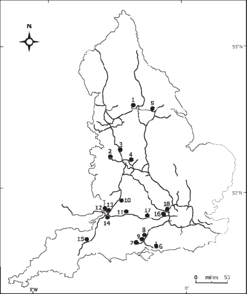
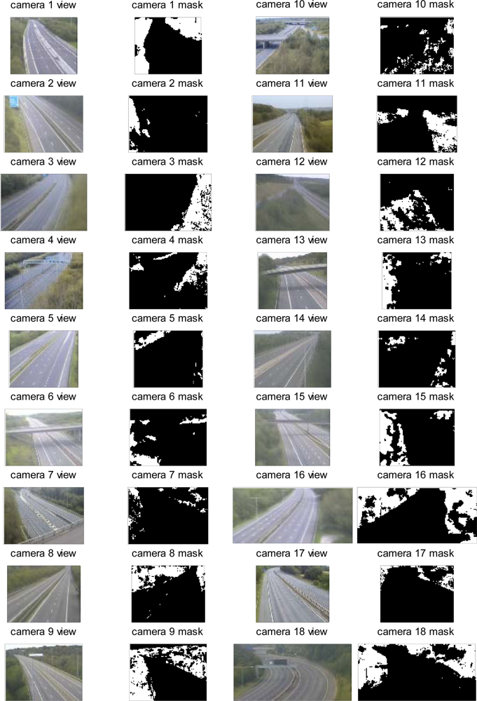
2. The Camera Network

The Highways Agency (HA) is an Executive Agency of the Department for Transport (DfT), and is responsible for operating, maintaining and improving the strategic road network in England on behalf of the UK’s Secretary of State for Transport [39]. The Agency maintains a high density network of traffic cameras deployed along its motorways and major trunk roads affording a continuous monitoring of traffic, and by default the vegetation that lines these roads and are within the field of view of the cameras. An agreement was made with the HA to access and download images from these cameras: three sets of images captured at 10:00, 12:00 and 14:00 local time were downloaded from the HA website daily. Cameras might not be available due to maintenance by HA, internet connectivity, and HA censorship due to incidents.

Access was granted to approximately 1,800 cameras in total and the size of each image varied between around 15 to 20 kB with the permitted download limit to an average bandwidth of 13 kB/s which means that it takes approximately half an hour for the images to download from all the cameras available due to the specified bandwidth limit. The digital images were downloaded and archived as heavily compressed JPEGs (352 × 288-pixel resolution, with three channels of 8-bit RGB colour information) for subsequent processing. Filenames included a date and time stamp for easy reference. A manual survey of the images captured by each camera revealed that 900 contained areas of vegetation suitable for the study. As a preliminary investigation, the present study was based on analysis of images recorded between 28 March 2011 and 5 December 2012. This paper focuses on images downloaded from 18 cameras located over a wide geographical spread and covering a range of vegetation types (Figure 1).

Table 1. Geographical location, elevation, direction of view and descriptions vegetation types in view of the cameras

No.	Latitude	Longitude	Elevation (m)	Direction	Vegetation Types
1	53.78°N	1.57°W	40	SW	Dense mixed hedgerow including hawthorn, with sycamore or maple, and oak trees.
2	52.69°N	2.50°W	132	ESE	Dense mature hedgerow 15 m high, with some coniferous trees.
3	52.83°N	2.15°W	98	NW	Dense mixed hedgerow 15 m high, with some hawthorn and ash trees.
4	52.51°N	1.76°W	105	W	Dense mixed hedgerow including hawthorn and blackthorn bushes.
5	53.61°N	0.98°W	6	NE	Mixed stand of trees containing sycamore, gorse, hawthorn, and conifer species.
6	50.91°N	1.00°W	69	S	Mixed stand of trees, all deciduous.
7	50.96°N	1.42°W	83	E	Dense mixed stand of conifer, ash, gorse and scots pine.
8	50.96°N	1.40°W	69	E	Dense mixed stand of gorse, ash, sycamore, and hawthorn.
9	51.08°N	1.29°W	51	NE	Dense mixed hedgerow in front of a tree line containing ash, conifer, oak, birch, gorse, sycamore.
10	51.86°N	2.17°W	46	NEN	Junction intersection: mixed level vegetation with individual trees including conifers, silver birch, and buckthorn.
11	51.51°N	2.08°W	71	E	Dense mixed stand of gorse, ash, sycamore, and hawthorn.
12	51.57°N	2.59°W	9	SE	Individual mature trees, including silver birch.
13	51.49°N	2.55°W	44	SW	Mixed scattered trees including blackthorn, ash and hawthorn.
14	51.51°N	2.66°W	8	NE	Dense mixed hedgerow ∼12–15 m high including hawthorn and blackthorn bushes.
15	50.98°N	3.14°W	70	WSW	Dense stands of mixed trees, containing willow, and maple.
16	51.50°N	0.70°W	24	NE	Dense stands of mixed trees, containing poplar, ash, and elder.
17	51.46°N	1.09°W	46	SE	Dense mixed trees including blackthorn, gorse and ash.
18	51.54°N	0.51°W	45	NE	Mixed trees including blackthorn, gorse and ash.

provides a summary of the characteristics at each camera site.

3. Methods

In order to develop an automated method for the extraction of phenological information from this network of traffic cameras there were several challenges to surmount. The first relates to the quality of each image that is dependent on a number of external factors, such as precipitation, insect activity or bird excrement on the lens. Further, vegetation may be obscured by road traffic at certain points in time. An additional challenge is that the framing of each individual image from a camera is variable, due to camera movement by wind or more significantly because a controller has changed where the camera is looking. As automation was desirable, a method that was scalable and transferable to other camera networks of this type was also a factor to consider. Accounting for these resulted in a three step approach from image capture to extraction of the phenological metrics desired: Step 1—Image pre-processing to collect images from cameras that are in the same general direction and align them; Step 2—identification of areas of the aligned images that have phenological interest for further analyses determination of the greenness of the areas determined over time; and Step 3—extraction of phenological metrics to be compared with manual inspection of the images.

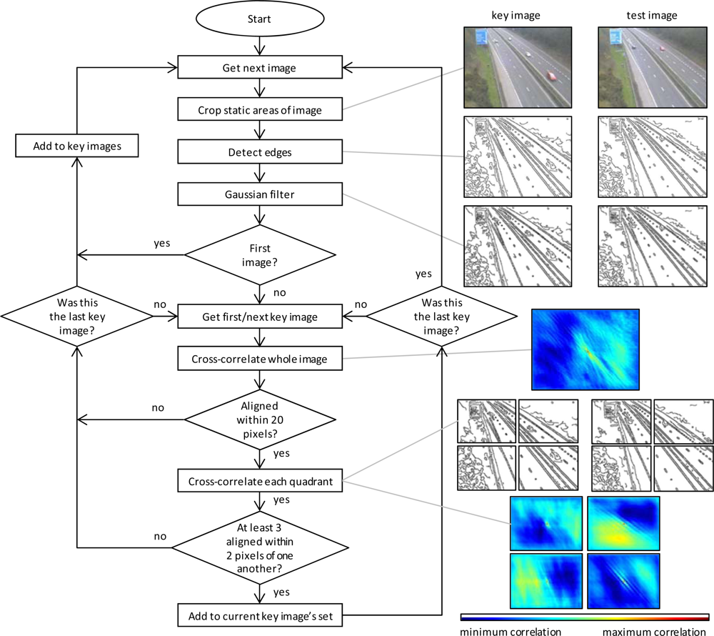
3.1. Image Pre-Processing

The cameras are under manual control by the Highways Agency and therefore the direction in which the cameras point is variable. The direction is dependent on road traffic conditions at the time and any incidents that may have occurred that require closer inspection by the relevant authorities. Cameras located away from junctions are more likely to be static for most of the time and are aimed looking down the highway rather than across it. The first step of processing is to automatically collect images from each camera into sets of images that were taken in the same general direction. This was performed by cropping all images to remove static ancillary information (such as overlaid timestamps generated by the camera). An initial key image (usually the first one in the set) was established and subsequently an attempt to align it with the remaining images from that camera (the test images) was made.

The alignment was not carried out on the raw images, but on ones that had been pre-processed. A binary image (two levels) describing where there were strong intensity edges within the image was found using an edge detector. This was then blurred with a Gaussian filter, which thickened the lines and gave them a Gaussian intensity profile. This was fed into a cross-correlation algorithm; the result of which generated a two-dimensional image, where the pixel intensities mapped how well aligned the two input images are if they were overlaid with different offsets between each another, in both the x- and y-axis. The offset between the maximum pixel value and the centre of the image was used to determine how much to offset one image against the other to bring them into alignment.

Any pair of images where the maximum of the cross-correlation image was within 20 pixels from the centre was considered to be part of the same set of images. The offset between the peak and the centre of the image represents how much to offset one image against the other to align them. A cross-correlation performed between any two images must always have a maximum point, even if the images have completely different compositions, furthermore, these maxima could be within 20 pixels from the centre by chance. This would have the effect of images appearing to be aligned when they were not. To avoid misalignments, each image was divided into four equal quadrants and cross-correlations performed on each quadrant independently. For the image to be taken as part of the same set, the offsets between at least three of the quadrants were required to be within 2 pixels of one another. If the key image was correlated within 20 pixels and passed the quadrant test then the tested image was added to the key image’s set. Otherwise, the image was treated as being taken in a different direction and became a new key image to be compared against later images. The process was repeated until all images were exhausted, by comparing each successive image with all the key images that had been determined so far. This process is also explained as a flowchart in Figure 2.

Because images were always tested over all previous key images, even if a match had been found, it was possible for some images to appear in more than one set. Intersecting sets were combined by calculating the mean offset of the images that were common to both sets (relative to the key images of each set) and shifting the offsets in each intersecting set relative to this, thus making a superset. As image alignment is part of the collation process, this also has the effect of removing small variations in the direction the camera was pointing in, due to the result of wind, for example. The process is resumable; the pre-processing stage can be restarted from where it last finished when newly acquired images are available, this means that the results can be continuously updated.

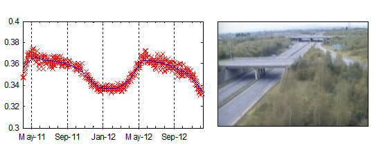
3.2. Determination of the Greenness of Pixels Containing Vegetation over Time

The common overlapping area was determined for each combined set and the excess was removed from each image. A value of greenness for the remaining pixels of each image in a set was then calculated using the following equation:

$$\text{greenness}=\frac{g}{r+g+b}$$

(1)

where: g, r, and b represent the raw green, red and blue values for each pixel [34]. This gives the proportion of the pixel’s overall intensity that is on the green channel and is therefore invariant to the overall brightness of the pixel. Since parts of the images in the set may not have been of use, either because they did not contain vegetation or because the vegetation was frequently obscured by passing traffic, areas of interest for each set of images were determined. A pixel was added to the area of interest if it had a phenological signature, that is, the greenness value rose in the spring and fell in the autumn. The greenness of each pixel in the time sequence was checked to see if it was greater or less than the mean greenness for that year (taken between the December solstices). Between the December solstice and the March equinox it was expected that the pixel value will be below the annual mean. Furthermore, between a month (28 days) before the June solstice and a month before the September equinox the pixel greenness was expected to be greater than the annual mean. For an area to be treated as having useful phenological information, the expectations needed to be met for over 99% of time points. A binary mask of pixels that fitted the conditions was created and applied to find the mean greenness value over all useful pixels at each time point.

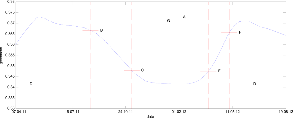
3.3. Extraction of Phenological Metrics

In order to extract dates relating to the onset of greenness (i.e., leaf up) and senescence (i.e., leaf fall) the series was smoothed using a local regression via weighted linear least squares and a first degree polynomial model (LOESS) with a span of 3 months (84 days) [40]. Phenological dates were extracted for each year of acquisition. The dates were found when the smoothed data: rose to 20% (beginning of leaf up season) and 80% (end of leaf up season) of the greenness range between the minimum and maximum greenness over the growing season; and when the greenness fell below 80% (start of senescence) and 20% (end of senescence) of the minimum and maximum greenness over the senescence season. An example of this is shown in Figure 3. Validation of the automatically extracted phenological dates was challenging, particularly since the greenness values are an aggregate of the whole scene captured by the camera which could contain several species with its own phenological cycle. Here, the image archive was used in a visual inspection validation process in order to provide an idea of the quality of the method outputs. Since the phenological curve is not complete for both years, only the end of senescence in 2011 and start of green-up in 2012 are evaluated.

4. Results

4.1. Assessment of Network Usability

Out of the 900 cameras deemed suitable for use, 72% of images provided sets from which phenological metrics could potentially be extracted automatically. The main reason for images being unsuitable for use included road structures (such as bridges) appearing too close to the camera; frequent motion in camera meaning that images available from the most frequently occurring camera angle are very sparse in temporal coverage; and large changes in camera angle which lead to low correlations between images in the temporal sequence. Although for illustrative purposes only 18 cameras are discussed in this paper, the 72% return would result in approximately 650 cameras and associated image sets for potential use. This represents a high density spatial coverage from which phenological information could be discovered to support research. It is acknowledged that there may be some micro-location effects in measurement of vegetation phenology at roadsides in the same way that micro-topography had an impact in the study by Fisher et al. [27]. Nevertheless, local processes are important to understand when scaling to regional representations such as those captured by satellite data [28]. As such this dataset represents an untapped potential particularly in a locality where high cloud coverage often precludes the construction of a high quality temporal time-series required for phenological measurement [41].

In each of the camera’s field of view the composition and distribution of the varied vegetation vary both in relation to the road and with each other; the method employed for the automatic extraction of areas of interest (i.e., vegetation) proved successful generally for the 18 cameras under scrutiny here as illustrated in Figure 4. In each case the road, street furniture, sky, areas frequently obscured by vehicles, and buildings are masked out leaving only the vegetation of interest. The proportion of masked areas differed from camera to camera but a visual inspection of each confirmed that the unmasked parts of the images were only vegetation. Further validation of this was provided by summing all of the images from a set which causes the cars to disappear gradually from the resulting image since their positions are randomly distributed along the roads within the image. This leaves only the constant objects such as the road, sky, trees, signs, buildings and street lamps. This procedure allowed the quality of the alignment of the images to be ascertained, with poorly aligned images looking blurred. This is the most crucial step with respect to camera usability. Other limiting factors in image quality via noise through environmental factors such as precipitation on the lens are ignored and accounted for via the smoothing of the high temporal frequency of image acquisition.

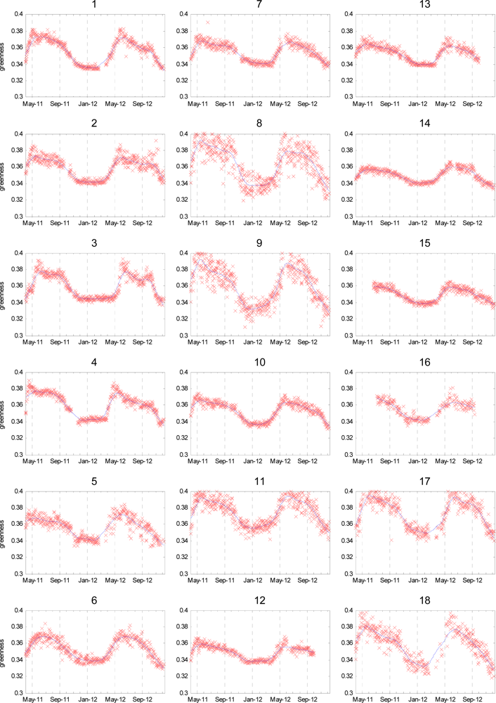
4.2. Extracted Time-Series Plots

The resultant time-series plot of the mean greenness value over all useful pixels is illustrated in Figure 5 for each camera.

Table 2. Quality indicators for the processed cameras.

No.	Vegetation Coverage on Image (%)	RMS Error on Fit to Time Series (× 10−3)	Valid Time-Points Present (% of Whole Sequence)
1	32.3	3.96	84.8
2	7.5	5.27	87.9
3	21.7	5.19	88.0
4	11.4	4.49	81.1
5	6.6	5.63	75.4
6	11.5	4.38	84.3
7	6.1	3.72	87.7
8	19.2	10.82	89.2
9	34.8	10.28	90.5
10	12.1	3.46	85.6
11	21.7	7.11	87.2
12	18.6	3.39	80.3
13	15.3	3.24	84.1
14	7.0	2.41	85.3
15	20.3	2.72	74.5
16	30.1	4.18	46.6
17	8.3	7.44	76.6
18	27.4	8.20	66.7

provides the root-mean-square (RMS) error on fit and the percentage of time-points present in time-series plots for each camera. It is evident that the plots are, unsurprisingly, inherently noisy, particularly those from cameras 8, 9, 11, 17 and 18, because of the uncontrolled conditions in which the images were taken. Furthermore there are missing data from some of the plots as a result of a step movement in the camera (for example from Camera 4 during the autumn of 2011). Despite this in each case there were enough data points available to parameterize a simple sigmoid-shaped model and extract the underlying signal. The missing data does however pose a challenge when visually extracting phenological dates and as such are excluded from further analyses (as per Section 4.3). The phenological signal is clearly well-defined for each camera. In most cases the classic trapezoid phenology profile is displayed and for both 2011 and 2012 there was a great similarity in the curves. In general terms, the greenness values are seen to increase rapidly from March/April, corresponding to a period of leafing-up mainly in the deciduous trees and increased photosynthetic activity in other vegetation types that had a strong enough phenological signal to be included in the area of interest (e.g., coniferous trees and some shrubs which maintain a minimum greenness during the winter months). The curve is seen to stabilize during June, followed by a rapid decrease in greenness from the end of August, marking the onset of the autumnal senescence. The curve reaches a minimum during the months of December to February. Since the signal extracted is an aggregate greenness value of all pixels in the area of interest, those cameras capturing scenes in which there is a higher proportion of deciduous vegetation (for example camera numbers 8, 9, 11 and 18) display a more pronounced seasonal curve due to large range in net primary productivity attained by this vegetation type. Where there are coniferous species in the scene, these will temper the range of greenness captured by the camera with a higher proportion of these since these species will not exhibit as large a seasonal variation in their photosynthetic biomass [42]. This concurs with other studies that have used camera-based indices for characterising canopy phenology [43].

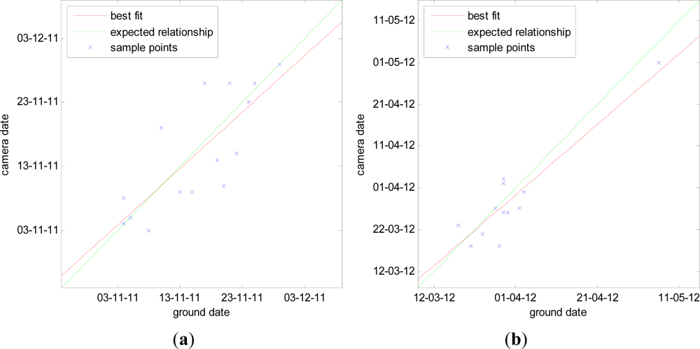
4.3. Computed Phenological Dates

The automated computed phenological event dates for all the 18 cameras for each year of investigation as indicated by the automatically extracted greenness values are presented in

Table 3. Automatically calculated phenological dates for the cameras that are shown Figure 1.

Camera No.	2011 Season		2012 Season
	Start of Senescence	End of Senescence	Start of Green-up	End of Green-up
1	28-Aug	08-Nov	14-Mar	09-May
2	19-Aug	04-Nov	27-Mar	05-May
3	07-Sep	05-Nov	01-May	01-Jun
4	25-Aug	05-Nov	18-Mar	22-Apr
5	30-Aug	09-Nov	02-Mar	28-Apr
6	17-Aug	03-Nov	26-Mar	09-May
7	26-Jul	26-Nov	03-Apr	16-May
8	07-Aug	15-Nov	02-Apr	09-May
9	26-Jun	10-Nov	23-Mar	10-May
10	25-Aug	26-Nov	21-Mar	02-May
11	16-Aug	09-Nov	27-Mar	12-May
12	30-Jul	14-Nov	26-Mar	30-Apr
13	12-Aug	29-Nov	18-Mar	27-Apr
14	08-Sep	26-Nov	23-Mar	02-May
15	21-Aug	07-Nov	01-Mar	02-May
16	30-Aug	20-Nov	18-Mar	03-May
17	18-Aug	19-Nov	31-Mar	22-May
18	13-Jul	23-Nov	06-Mar	11-May

. Figure 6 shows a comparison between the date of end of senescence for 2011 and start of leaf-up for 2012 observed through the automated method and visual inspection validation dates across the 18 cameras. In both cases a strong Pearson’s correlation coefficient, r, was found (r = 0.7879, p < 0.001, date of end of senescence, 2011; r = 0. 9199, p < 0.001, date of end of start of leaf-up, 2012). Although the automated analysis estimated dates too early compared with visual inspection of the cameras’ images, and others too late, overall the root-mean-square difference between the estimate dates using the automated and manual methods was five days. Compared with the date of start of green up, the date of end of senescence was less certain. This concurs with other studies (using satellite data) that suggest it is more challenging to measure this as a single date [44] but that this can be overcome using a different index of the data (e.g., green-red vegetation index (GRVI) [45]). In order to fully understand why there was error in the predicted dates the values of greenness would need disaggregating to the component vegetation types and further research into different methods of data smoothing and date extraction would be required (similar to that applied to satellite data [29,46]).

5. Discussion

The results obtained in this pilot study are encouraging. It is suggested that the methods for using the images captured by these traffic cameras are refined and in doing so the ecological value of these data will be fully realised. The data could benefit a multi-scale monitoring programme of phenology so critical for an improved understanding of environmental change, in particular that associated with climate variability [13]. The continuous measurement of phenology at high temporal and spatial resolution affords an understanding of trends in vegetation productivity and this could be achieved via aggregation across multiple species or for specific species in selected locations [47]. The ability to focus on species is possible via the manual extraction of areas of interest and would allow a better understanding of the seasonal-gap that exists between species [48], as well as the role of site-specific properties and geographical location [49]. The images captured by these traffic cameras offer extended analysis possibilities, particularly when coupled with similar resolution observations of precipitation and temperature, carbon flux measurements and soil properties [47]. This will benefit the understanding of budgets of carbon and water exchange (e.g., gross primary productivity (GPP) [50,51]) and moreover shed light on any interannual variability in the growing season caused by weather conditions (e.g., windstorms [52]) and other occasional but often severe biotic stresses that influence the physiological status of trees [45,53]. Beyond this there is scope for the data to be used in the understanding of ecosystem interactions, food chains, pollination, breeding and migration [54,55].

Using a network such as that offered here meets the requirements for a spatially dense set of observations that are geographically widespread but comply with standardised rules [36]. Cameras fill in the large scale-gap that exists between observers who tend to focus on one tree and the satellite-derived data which are useful at the ecosystem scale [50]. From a UK perspective, this network could be well placed to understand the impact of current observed trends in the climate on its vegetation: the Central England Temperature has risen by about 1 °C since the 1970s, with 2006 being the warmest in the 348-year long record. Seasonal rainfall is highly variable, but there has been a slight trend over the last 250 years for decreased rainfall in summer and increased in winter [56]. Any environmental impacts already evident are likely to be exacerbated in the near future given climate change projections [57,58] which indicate that the UK climate will continue to warm substantially and that increases in the number of days with high temperatures will be found everywhere, particularly in south east England. Further, reductions in the number of frost days are predicted, as well as increases in the number of 10-day dry spells across the UK, this being more pronounced in southern England and in Wales. There will also be further changes in rainfall patterns and its seasonal distribution; and considerable regional variations can be expected. A detailed study into the observed impacts of climate change on UK vegetation to date found that there is clear evidence that climate change is having an impact on some aspects of the composition and function of woodland [59]. Leafing has advanced by 2–3 weeks since the 1950s. However, evidence for increases in tree growth rates and forest productivity resulting from lengthening growing seasons is limited for the UK, yet the link between climate change, primary productivity and growing season has been evident elsewhere [60]. Current records of CO₂ fluxes between forests and the tropospheric atmosphere are limited to two sites, which do not allow the full heterogeneity of UK trees to be accounted for and are therefore insufficient for a full-evidence based management system to support policy decisions on how forests are used in climate change mitigation.

Although further work is to be conducted using this network of cameras, this study joins others who have used cameras to capture leaf emergence and green-up (e.g., [34,50,53]) as well as senescence (e.g., [36,50]). Such studies point to the possibility of using other combinations of spectral channels (e.g., Zhao et al. computed a redness index [36]; Mizunuma et al. used a Hue value [51], with Motohka et al. recommending the GRVI [45]). Other suggested research avenues include a focus on understorey vegetation [16,61], though this would not be directly applicable using this network, though at different times of year the leaf area of certain trees may allow “background” vegetation to be observed [48,50]. Another avenue could be to examine the variability in the accuracy with which the phenological dates are captured as a function of the timing of the images used. In this study only the data captured at 12 noon was processed similar to others [25,34,50,53], however, it has been noted that images captured earlier and later than midday better characterise the phenological pattern of plant species using machine learning [62], which the currently unused data collected at 10am and 2pm could be applied to in future.

6. Conclusions

This paper describes the first attempt at fully automatically extracting plant phenological metrics from a web-hosted system of traffic cameras. The results obtained demonstrate that a well-defined signal related to spring green-up and autumn senescence can be extracted from the images recorded, illustrating that valuable information complementary to their primary purpose can be obtained from such networks. Key to the method presented here is that vegetation with a phenological signal is found automatically with no human intervention required. Furthermore, the method is robust with respect to camera movement and so not subject to as greater loss of data as seen in a previous study [28].

Since the method presented in this paper is scalable and transferable it could be applied globally and coupled with other cameras of this nature (e.g., CCTV in urban areas). Internet searches have confirmed that most countries possessing extensive road networks make use of a corresponding camera network to monitor traffic flow. Therefore the approach described here could in principle be applied globally at minimal cost, greatly benefiting from both the initial camera installation and the on-going maintenance being handled by the road network operators. There is a real potential to roll this out within a systematic and scientifically credible monitoring programme achieving a spatial resolution and coverage not previously achieved.

Although this paper demonstrates the method, further work is required: to perform a fuller validation and to better understand the nature of the errors that will be present; and to investigate the application of methods and image selection to refine the approach. With the passing years there will be real value in utilising this image archive to understand drivers of phenological trends, coupling extracted metrics with other data. To do this would add further support to the potential use of traffic cameras for the measurement of phenology; particularly within a scheme to validate satellite data by way of increasing the spatial extent and sampling rate [28]; pertinent since the imminent launch of Earth observation systems such as the Sentinels have an improved temporal resolution meaning that ground based validation is of increasing importance [63]. Moreover, the use of traffic cameras fills a scale-gap between other approaches to measuring phenology and it is suggested that consideration be given to a multiple-system approach that incorporates all approximations of phenology (i.e., satellite, airborne, terrestrial, citizen based) and overcomes the limitations of each one [64].

References

1. Richardson, A.D.; Anderson, R.S.; Arain, M.A.; Barr, A.G.; Bohrer, G.; Chen, G.S.; Chen, J.M.; Ciais, P.; Davis, K.J.; Desai, A.R.; et al. Terrestrial biosphere models need better representation of vegetation phenology: Results from the North American Carbon Program Site Synthesis. Glob. Change Biol. 2012, 18, 566–584. [Google Scholar]
2. Schwartz, M.D.; Betancourt, J.L.; Weltzin, J.F. From Caprio’s lilacs to the USA national phenology network. Front. Ecol. Environ. 2012, 10, 324–327. [Google Scholar]
3. Brügger, R.; Dobbertin, M.; Kräuchi, N. Phenological Variation of Forest Trees. In Phenology: An Integrative Environmental Science; Schwartz, M., Ed.; Kluwer Academic Publishers: Dordrecht, The Netherlands, 2003; Volume 39, pp. 255–267. [Google Scholar]
4. Molod, A.; Salmun, H.; Waugh, D.W. A new look at modeling surface heterogeneity: Extending its influence in the vertical. J. Hydrometeorol. 2003, 4, 810–825. [Google Scholar]
5. Wilson, K.B.; Baldocchi, D.D. Seasonal and interannual variability of energy fluxes over a broadleaved temperate deciduous forest in North America. Agric. For. Meteorol. 2000, 100, 1–18. [Google Scholar]
6. Cleland, E.E.; Chuine, I.; Menzel, A.; Mooney, H.A.; Schwartz, M.D. Shifting plant phenology in response to global change. Trends Ecol. Evol. 2007, 22, 357–365. [Google Scholar]
7. Richardson, A.D.; Black, T.A.; Ciais, P.; Delbart, N.; Friedl, M.A.; Gobron, N.; Hollinger, D.Y.; Kutsch, W.L.; Longdoz, B.; Luyssaert, S.; et al. Influence of spring and autumn phenological transitions on forest ecosystem productivity. Philos. Trans. R. Soc. B Biol. Sci. 2010, 365, 3227–3246. [Google Scholar] [Green Version]
8. Lucht, W.; Prentice, I.C.; Myneni, R.B.; Sitch, S.; Friedlingstein, P.; Cramer, W.; Bousquet, P.; Buermann, W.; Smith, B. Climatic control of the high-latitude vegetation greening trend and pinatubo effect. Science 2002, 296, 1687–1689. [Google Scholar]
9. Betts, R.A. Offset of the potential carbon sink from boreal forestation by decreases in surface albedo. Nature 2000, 408, 187–190. [Google Scholar]
10. Doi, H.; Takahashi, M. Latitudinal patterns in the phenological responses of leaf colouring and leaf fall to climate change in Japan. Glob. Ecol. Biogeogr. 2008, 17, 556–561. [Google Scholar]
11. Badeck, F.W.; Bondeau, A.; Bottcher, K.; Doktor, D.; Lucht, W.; Schaber, J.; Sitch, S. Responses of spring phenology to climate change. New Phytol. 2004, 162, 295–309. [Google Scholar]
12. Migliavacca, M.; Galvagno, M.; Cremonese, E.; Rossini, M.; Meroni, M.; Sonnentag, O.; Cogliati, S.; Manca, G.; Diotri, F.; Busetto, L.; et al. Using digital repeat photography and eddy covariance data to model grassland phenology and photosynthetic CO2 uptake. Agric. For. Meteorol. 2011, 151, 1325–1337. [Google Scholar]
13. Wingate, L.; Richardson, A.D.; Weltzin, J.F.; Nasahara, K.N.; Grace, J. Keeping an eye on the carbon balance: Linking canopy development and net ecosystem exchange using a webcam. FluxLette 2008, 1, 14–17. [Google Scholar]
14. Morisette, J.T.; Richardson, A.D.; Knapp, A.K.; Fisher, J.I.; Graham, E.A.; Abatzoglou, J.; Wilson, B.E.; Breshears, D.D.; Henebry, G.M.; Hanes, J.M.; et al. Tracking the rhythm of the seasons in the face of global change: Phenological research in the 21st century. Front. Ecol. Environ. 2009, 7, 253–260. [Google Scholar]
15. Graham, E.A.; Yuen, E.M.; Robertson, G.F.; Kaiser, W.J.; Hamilton, M.P.; Rundel, P.W. Budburst and leaf area expansion measured with a novel mobile camera system and simple color thresholding. Environ. Exp. Bot. 2009, 65, 238–244. [Google Scholar]
16. Liang, L.A.; Schwartz, M.D.; Fei, S.L. Validating satellite phenology through intensive ground observation and landscape scaling in a mixed seasonal forest. Remote Sens. Environ. 2011, 115, 143–157. [Google Scholar]
17. Garrity, S.R.; Bohrer, G.; Maurer, K.D.; Mueller, K.L.; Vogel, C.S.; Curtis, P.S. A comparison of multiple phenology data sources for estimating seasonal transitions in deciduous forest carbon exchange. Agric. For. Meteorol. 2011, 151, 1741–1752. [Google Scholar]
18. White, J.W.; Kimball, B.A.; Wall, G.W.; Ottman, M.J.; Hunt, L.A. Responses of time of anthesis and maturity to sowing dates and infrared warming in spring wheat. Field Crops Res. 2011, 124, 213–222. [Google Scholar]
19. Studer, S.; Stockli, R.; Appenzeller, C.; Vidale, P.L. A comparative study of satellite and ground-based phenology. Int. J. Biometeorol. 2007, 51, 405–414. [Google Scholar]
20. Sonnentag, O.; Hufkens, K.; Teshera-Sterne, C.; Young, A.M.; Friedl, M.; Braswell, B.H.; Milliman, T.; O’Keefe, J.; Richardson, A.D. Digital repeat photography for phenological research in forest ecosystems. Agric. For. Meteorol. 2012, 152, 159–177. [Google Scholar]
21. Betancourt, J.L.; Schwartz, M.D.; Breshears, D.D.; Brewer, C.A.; Frazer, G.; Gross, J.E.; Mazer, S.J.; Reed, B.C.; Wilson, B.E. Evolving plans for the USA National Phenology Network. Eos Trans. AGU 2007, 88, 211. [Google Scholar]
22. Collinson, N.; Sparks, T. Phenology—Nature’s calendar: An overview of results from the UK phenology network. Arboric. J. 2008, 30, 271–278. [Google Scholar]
23. Jenkins, J.P.; Richardson, A.D.; Braswell, B.H.; Ollinger, S.V.; Hollinger, D.Y.; Smith, M.L. Refining light-use efficiency calculations for a deciduous forest canopy using simultaneous tower-based carbon flux and radiometric measurements. Agric. For. Meteorol. 2007, 143, 64–79. [Google Scholar]
24. Wang, Z.J.; Wang, J.H.; Liu, L.Y.; Huang, W.J.; Zhao, C.J.; Wang, C.Z. Prediction of grain protein content in winter wheat (Triticum aestivum L.) using plant pigment ratio (PPR). Field Crops Res. 2004, 90, 311–321. [Google Scholar]
25. Richardson, A.D.; Braswell, B.H.; Hollinger, D.Y.; Jenkins, J.P.; Ollinger, S.V. Near-surface remote sensing of spatial and temporal variation in canopy phenology. Ecol. Appl. 2009, 19, 1417–1428. [Google Scholar]
26. Boyd, D.S.; Almond, S.; Dash, J.; Curran, P.J.; Hill, R.A. Phenology of vegetation in Southern England from Envisat MERIS terrestrial chlorophyll index (MTCI) data. Int. J. Remote Sens. 2011, 32, 8421–8447. [Google Scholar]
27. Fisher, J.I.; Mustard, J.F.; Vadeboncoeur, M.A. Green leaf phenology at Landsat resolution: Scaling from the field to the satellite. Remote Sens. Environ. 2006, 100, 265–279. [Google Scholar]
28. Graham, E.A.; Riordan, E.C.; Yuen, E.M.; Estrin, D.; Rundel, P.W. Public internet-connected cameras used as a cross-continental ground-based plant phenology monitoring system. Glob. Change Biol. 2010, 16, 3014–3023. [Google Scholar]
29. Eklundh, L.; Jin, H.X.; Schubert, P.; Guzinski, R.; Heliasz, M. An optical sensor network for vegetation phenology monitoring and satellite data calibration. Sensors 2011, 11, 7678–7709. [Google Scholar]
30. Fisher, J.I.; Mustard, J.F. Cross-scalar satellite phenology from ground, Landsat, and MODIS data. Remote Sens. Environ. 2007, 109, 261–273. [Google Scholar]
31. Fisher, J.I.; Richardson, A.D.; Mustard, J.F. Phenology model from surface meteorology does not capture satellite-based greenup estimations. Glob. Change Biol. 2007, 13, 707–721. [Google Scholar]
32. Boyd, C.S.; Svejcar, T.J. A visual obstruction technique for photo monitoring of willow clumps. Rangel. Ecol. Manag. 2005, 58, 434–438. [Google Scholar]
33. Slaughter, D.C.; Giles, D.K.; Downey, D. Autonomous robotic weed control systems: A review. Comput. Electron. Agric. 2008, 61, 63–78. [Google Scholar]
34. Richardson, A.D.; Jenkins, J.P.; Braswell, B.H.; Hollinger, D.Y.; Ollinger, S.V.; Smith, M.L. Use of digital webcam images to track spring green-up in a deciduous broadleaf forest. Oecologia 2007, 152, 323–334. [Google Scholar]
35. Crimmins, M.A.; Crimmins, T.M. Monitoring plant phenology using digital repeat photography. Environ. Manage. 2008, 41, 949–958. [Google Scholar]
36. Zhao, J.B.; Zhang, Y.P.; Tan, Z.H.; Song, Q.H.; Liang, N.S.; Yu, L.; Zhao, J.F. Using digital cameras for comparative phenological monitoring in an evergreen broad-leaved forest and a seasonal rain forest. Ecol. Inform. 2012, 10, 65–72. [Google Scholar]
37. Hufkens, K.; Friedl, M.; Sonnentag, O.; Braswell, B.H.; Milliman, T.; Richardson, A.D. Linking near-surface and satellite remote sensing measurements of deciduous broadleaf forest phenology. Remote Sens. Environ. 2012, 117, 307–321. [Google Scholar]
38. Li, H.F.; Fu, X.S. An intelligence traffic accidence monitor system using sensor web enablement. Procedia Eng. 2011, 15, 2098–2102. [Google Scholar]
39. Highways Agency. Avaiable online: http://www.highways.gov.uk/about-us/what-we-do/ (accessed on 9 November 2012).
40. Cleveland, W.S.; Devlin, S.J. Locally weighted regression—An approach to regression-analysis by local fitting. J. Am. Stat. Assoc. 1988, 83, 596–610. [Google Scholar]
41. Armitage, R.P.; Alberto Ramirez, F.; Mark Danson, F.; Ogunbadewa, E.Y. Probability of cloud-free observation conditions across Great Britain estimated using MODIS cloud mask. Remote Sens. Lett. 2012, 4, 427–435. [Google Scholar]
42. Kimball, J.S.; McDonald, K.C.; Running, S.W.; Frolking, S.E. Satellite radar remote sensing of seasonal growing seasons for boreal and subalpine evergreen forests. Remote Sens. Environ. 2004, 90, 243–258. [Google Scholar]
43. Saitoh, T.M.; Nagai, S.; Saigusa, N.; Kobayashi, H.; Suzuki, R.; Nasahara, K.N.; Muraoka, H. Assessing the use of camera-based indices for characterizing canopy phenology in relation to gross primary production in a deciduous broad-leaved and an evergreen coniferous forest in Japan. Ecol. Inform. 2012, 11, 45–54. [Google Scholar]
44. Nagai, S.; Maeda, T.; Gamo, M.; Muraoka, H.; Suzuki, R.; Nasahara, K.N. Using digital camera images to detect canopy condition of deciduous broad-leaved trees. Plant Ecol. Div. 2011, 4, 79–89. [Google Scholar]
45. Motohka, T.; Nasahara, K.N.; Oguma, H.; Tsuchida, S. Applicability of green-red vegetation index for remote sensing of vegetation phenology. Remote Sens. 2010, 2, 2369–2387. [Google Scholar]
46. Atkinson, P.M.; Jeganathan, C.; Dash, J.; Atzberger, C. Inter-comparison of four models for smoothing satellite sensor time-series data to estimate vegetation phenology. Remote Sens. Environ. 2012, 123, 400–417. [Google Scholar]
47. Schwartz, M.D.; Hanes, J.M.; Liang, L. Comparing carbon flux and high-resolution spring phenological measurements in a northern mixed forest. Agric. For. Meteorol. 2013, 169, 136–147. [Google Scholar]
48. Nasahara, K.N.; Muraoka, H.; Nagai, S.; Mikami, H. Vertical integration of leaf area index in a Japanese deciduous broad-leaved forest. Agric. For. Meteorol. 2008, 148, 1136–1146. [Google Scholar] [Green Version]
49. Schleip, C.; Sparks, T.H.; Estrella, N.; Menzel, A. Spatial variation in onset dates and trends in phenology across Europe. Climate Res. 2009, 39, 249–260. [Google Scholar]
50. Ahrends, H.E.; Etzold, S.; Kutsch, W.L.; Stoeckli, R.; Bruegger, R.; Jeanneret, F.; Wanner, H.; Buchmann, N.; Eugster, W. Tree phenology and carbon dioxide fluxes: Use of digital photography at for process-based interpretation the ecosystem scale. Climate Res. 2009, 39, 261–274. [Google Scholar]
51. Mizunuma, T.; Wilkinson, M.; Eaton, E.L.; Mencuccini, M.; Morison, J.I.L.; Grace, J. The relationship between carbon dioxide uptake and canopy colour from two camera systems in a deciduous forest in southern England. Funct. Ecol. 2013, 27, 196–207. [Google Scholar]
52. Ryu, Y.; Verfaillie, J.; Macfarlane, C.; Kobayashi, H.; Sonnentag, O.; Vargas, R.; Ma, S.; Baldocchi, D.D. Continuous observation of tree leaf area index at ecosystem scale using upward-pointing digital cameras. Remote Sens. Environ. 2012, 126, 116–125. [Google Scholar]
53. Ide, R.; Oguma, H. Use of digital cameras for phenological observations. Ecol. Inform. 2010, 5, 339–347. [Google Scholar]
54. Bater, C.W.; Coops, N.C.; Wulder, M.A.; Nielsen, S.E.; McDermid, G.; Stenhouse, G.B. Design and installation of a camera network across an elevation gradient for habitat assessment. Instrum. Sci. Technol. 2011, 39, 231–247. [Google Scholar]
55. Doi, H.; Gordo, O.; Katano, I. Heterogeneous intra-annual climatic changes drive different phenological responses at two trophic levels. Climate Res. 2008, 36, 181–190. [Google Scholar]
56. Jenkins, G.; Perry, M.; Prior, J. UKCIP08: The Climate of the United Kingdom and Recent Trends; Meteorological Office Hadley Centre: Exeter, UK, 2009. [Google Scholar]
57. Lamb, R. UKCP 09-UK Climate Projections 2009; Oxford University: Oxford, UK, 2010. [Google Scholar]
58. Murphy, J.; Sexton, D.; Jenkins, G.; Booth, B.; Brown, C.; Clark, R.; Collins, M.; Harris, G.; Kendon, E.; Betts, R. UK Climate Projections Science Report: Climate Change Projections; Meteorological Office Hadley Centre: Exeter, UK, 2009. [Google Scholar]
59. Broadmeadow, M.; Morecroft, M.; Morison, J. Observed Impacts of Climate Change on UK Forests to Date. In Combating Climate Change: A Role for UK Forests. An Assessment of the Potential of the UK's Trees and Woodlands to Mitigate and Adapt to Climate Change; Read, D., Freer-Smith, P., Hanley, N., West, C., Snowdon, P., Eds.; The Stationery Office Limited: Norwich, UK, 2009; pp. 50–66. [Google Scholar]
60. Graham, E.A.; Yuen, E.M.; Robertson, G.F.; Kaiser, W.J.; Hamilton, M.P.; Rundel, P.W. Budburst and leaf area expansion measured with a novel mobile camera system and simple color thresholding. Environ. Exp. Bot. 2009, 65, 238–244. [Google Scholar]
61. Bater, C.W.; Coops, N.C.; Wulder, M.A.; Hilker, T.; Nielsen, S.E.; McDermid, G.; Stenhouse, G.B. Using digital time-lapse cameras to monitor species-specific understorey and overstorey phenology in support of wildlife habitat assessment. Environ. Monit. Assess. 2011, 180, 1–13. [Google Scholar]
62. Almeida, J.; dos Santos, J.A.; Alberton, B.; Torres, R.D.; Morellato, L.P.C. Remote Phenology: Applying Machine Learning to Detect Phenological Patterns in a Cerrado Savanna. Proceedings of 2012 IEEE 8th International Conference on E-Science (E-Science), Chicago, IL, USA, 8–12 October 2012.
63. Berger, M.; Moreno, J.; Johannessen, J.A.; Levelt, P.F.; Hanssen, R.F. ESA’s sentinel missions in support of Earth system science. Remote Sens. Environ. 2012, 120, 84–90. [Google Scholar]
64. Polgar, C.A.; Primack, R.B. Leaf-out phenology of temperate woody plants: From trees to ecosystems. New Phytol. 2011, 191, 926–941. [Google Scholar]
Figure 1. Map of England showing locations of the cameras used for the results shown in this paper. The bold lines represent the roads covered by Highways Agency cameras.
Remotesensing 05 02200f1
Figure 2. Flow-chart describing the image collection and alignment process, along with example images output at different stages of the process.
Remotesensing 05 02200f2
Figure 3. Graphical description of the determination of phenological dates. A, season maximum; B, start of senescence, 80% between D and A; C, end of senescence, 20% between D and A; D, inter-seasonal minimum; E, start of leaf-up, 20% between D and G; F, end of leaf up, 80% between D and G; G, season maximum. Vertical lines show intersections for date read-off.
Remotesensing 05 02200f3
Figure 4. Views of the cameras shown in Figure 1, after realignment and averaging over all images with corresponding calculated masks (white) of vegetation used for analysis.
Remotesensing 05 02200f4
Figure 5. Calculated greenness levels using Equation (1) for each camera shown in Figure 1 over the period of analysis. The crosses show individual data points and the continuous curves show the smoothed data used for date extraction.
Remotesensing 05 02200f5
Figure 6. Ground truth dates versus dates automatically calculated from cameras; (a) end of senescence 2011; (b) start of green up 2012. Note: missing points are due to lack of camera data for visual inspection.
Remotesensing 05 02200f6