Image-Based Coral Reef Classification and Thematic Mapping
by
A.S.M. Shihavuddin
1,*, 
Nuno Gracias
1,
Rafael Garcia
1,
Arthur C. R. Gleason
2 and
Brooke Gintert
3 1
Computer Vision and Robotics Group, Universitat de Girona, Campus Montilivi, Edifici P-IV, E-17071 Girona, Spain
2
Department of Physics, University of Miami, 1320 Campo Sano Ave., Coral Gables, FL 33146, USA
3
Department of Marine Geology and Geophysics, University of Miami, Rickenbacker Causeway, Coral Gables, FL 33146, USA
*
Author to whom correspondence should be addressed.
Remote Sens. 2013, 5(4), 1809-1841; https://doi.org/10.3390/rs5041809
Submission received: 21 February 2013
/
Revised: 29 March 2013
/
Accepted: 31 March 2013
/
Published: 15 April 2013
(This article belongs to the Special Issue Remote Sensing for Understanding Coral Reef Dynamics and Processes: Photo-Systems to Coral Reef Systems)
Abstract
:This paper presents a novel image classification scheme for benthic coral reef images that can be applied to both single image and composite mosaic datasets. The proposed method can be configured to the characteristics (e.g., the size of the dataset, number of classes, resolution of the samples, color information availability, class types, etc.) of individual datasets. The proposed method uses completed local binary pattern (CLBP), grey level co-occurrence matrix (GLCM), Gabor filter response, and opponent angle and hue channel color histograms as feature descriptors. For classification, either k-nearest neighbor (KNN), neural network (NN), support vector machine (SVM) or probability density weighted mean distance (PDWMD) is used. The combination of features and classifiers that attains the best results is presented together with the guidelines for selection. The accuracy and efficiency of our proposed method are compared with other state-of-the-art techniques using three benthic and three texture datasets. The proposed method achieves the highest overall classification accuracy of any of the tested methods and has moderate execution time. Finally, the proposed classification scheme is applied to a large-scale image mosaic of the Red Sea to create a completely classified thematic map of the reef benthos.
Keywords:
automated coral reef classification; benthic habitat classification; optical imagery; texture feature; kernel mapping; support vector machine; opponent angle; thematic mapping; optical mapping; probability density weighted mean distance; local binary pattern; grey level co-occurrence matrix; low resolution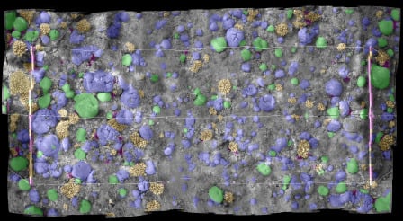
1. Introduction
For many, the term “remote sensing” is synonymous with satellite imagery or perhaps satellite and aerial imagery. Remote sensing, thus defined, implies a platform (overhead), a technology (usually passive optics) and a spatial scale (m to km pixels, regional to global extent). More broadly, however, remote sensing includes any method of detection or measurement made without directly contacting the object of study. Several technologies that are relevant for coral reef remote sensing, such as single- or multi-beam sonars, for example, fall under a more inclusive definition of remote sensing.
Underwater imagery is another remote sensing technology that has been used in virtually every aspect of marine science. In particular, images of the seabed have become vital tools for exploration, archaeology, marine geology and marine biology, among other fields. Underwater images, like terrestrial, hand-held images, tend to be overlooked even with a broad definition of “remote sensing”, yet they complement satellite, airborne and ship-based sensors by providing information at finer spatial resolution (< mm to cm scale pixels), albeit over a smaller area per image or per unit time of data collection.
The high spatial resolution afforded by underwater imagery of the seabed is fundamentally different from satellite, aerial and ship-borne sensors in the sense that images taken close to the seabed may be categorized as methods of direct remote sensing for the study of coral reef biodiversity (Turner et al. [1]). Direct remote sensing means that the actual individuals being studied (benthic organisms in this case) can be resolved. Overhead imagery and acoustic mapping, in contrast, are indirect methods for study in coral reef biology and ecology, because, rather than resolving individual organisms, they quantify proxies of biodiversity or they correlate with in situ measurements (Turner et al. [1]).
Direct remote sensing of the seabed complements indirect methods of coral reef remote sensing, because it allows different types of measurements to be made. For example, species identification for many benthic organisms is possible from underwater images, so species diversity indices can be calculated. Sizes of individual coral colonies can be measured and tracked through time. The fate of individuals impacted by bleaching or disease can be tracked through time. Many other uses for the imagery can be imagined, but in general, such measurements are infrequently used, due to two obstacles. First, until recently, it was difficult to obtain large numbers of seabed images across large enough areas to create statistically viable sample sizes. Second, extraction of quantitative information from seabed images is a laborious task that requires a significant time commitment of expert analysts.
Two technological advancements in the early 2000s qualitatively changed the acquisition of underwater imagery. One development was the widespread availability of digital, consumer-level still and video cameras. Digital cameras, along with associated advancements in batteries and storage, have largely removed constraints on the quantity of images that can be acquired. In 2000, a SCUBA diver with a Nikonos underwater camera was limited to 36 photographs per dive, but in 2013, the same diver with a digital camera can capture literally thousands of images in a single dive. The second development was the increased sophistication and availability of platforms, such as remotely operated vehicles (ROVs), autonomous underwater vehicles (AUVs) and towed bodies. These new platforms allow image capture at depths and across spatial scales that are not possible with divers or practical (for expense reasons) with manned submersibles.
Advancements in underwater image acquisition have largely removed the first obstacle to fully exploiting seabed images for coral reef remote sensing, but, ironically, they have exacerbated the second. It is now easy and common to collect more imagery during reef surveys that can be practically analyzed by hand. Nevertheless, images of reef surveys are useless to understanding reef processes unless examined by an expert analyst. Software packages, such as CPCe [2], have facilitated the transfer of information from imagery to analysis; however, humans are still “in the loop.”
An automated process for classifying underwater optical imagery would enhance the study of coral reef dynamics and processes by reducing the analysis bottleneck and allowing researchers to take full advantage of large underwater image datasets. Efforts to automate classification have been made for well over a decade [3], but no single algorithm is yet widely accepted as robust. A few of the most challenging obstacles to classification accuracy in coral reef environments include: significant intra-class and inter-site variability in the morphology of benthic organisms [4], complex spatial borders between classes on the seabed, subjective annotation of training data by different analysts, variation in viewpoints, distances and image quality, limits to spatial and spectral resolution when trying to classify to a free taxonomic scale, partial occlusion of objects due to the three-dimensional structure of the seabed, lighting artifacts due to wave focusing [5–7] and variable optical properties of the water column.
The existing methods for coral reef image classification have been tested on unique image datasets within the papers in which they were published; their utility has not been demonstrated on common datasets. Without comparison on standard datasets, it is impossible to assess the relative effectiveness and efficiency of these methods: Pizarro [8], Beijbom [4], Marcos [9] and Stokes and Deane [10]. All the previous algorithms used fixed classification schemes for all types of underwater optical image datasets. In general, however, characteristics, such as the size, number, resolution and color information of the images, vary from dataset to dataset. Therefore, a fixed recipe for automated classification for all types of optical image datasets might not always provide the best solution.
The goals of this work are to develop an improved method for classifying underwater optical images of coral reefs and to compare the proposed method with existing alternative approaches. The main difference of this new method, relative to previous algorithms, is that classification schemes should be malleable depending on the characteristics of each dataset (e.g., the size of the dataset, number of classes, resolution of the samples, color information availability, class types, etc.). In the proposed method, different combinations of features and classifiers are tuned to each dataset prior to classification to increase classification accuracy. Our new method is compared with the existing algorithms for accuracy and time requirement on six image datasets (Section 4). Finally, image classification methods were applied to a composite mosaic image to demonstrate the applicability of this approach for images that cover areas larger than a single image.
2. Review of Existing Algorithms for Automated Benthic Classification Using Optical Imagery
A short summary of existing algorithms for automated benthic classification using optical imagery is given in Table 1, with entries in bold corresponding to the published methods tested in Sections 4 and 5 of this paper.
Only published methods that exclusively used optical imagery and produced accurate multi-class classifications were chosen for comparison against the proposed classification scheme. Among these works, Marcos [9] used mean hue-saturation value (HSV) or normalized chromaticity coordinate (NCC) color features, which in many cases, are not discriminative enough for classification among classes. In the work of Pizarro [8], an entire image is classified as one class. Therefore, within-image heterogeneity cannot be classified or quantified. The method by Stokes and Deane [10] is time-efficient; however, the weighting of the color and texture features during feature vector creation were done manually. Beijbom [4] used multiple patch sizes; therefore, features in the patch are calculated several times, which is redundant and time-consuming.
Much additional work has been done on texture classification for other applications besides benthic imagery. Two papers in particular are worth mentioning here, as they reported the highest classification accuracy on standard texture datasets. Caputo [19] used filter bank outputs with a support vector machine (SVM) classifier that had a kernel based on the chi-square distance. This method worked very effectively on low-resolution texture datasets. Zhang [20] used an approach that represents images as distributions (signatures or histograms) of features extracted from a sparse set of key points locations and trained a SVM classifier with kernels based on the earth mover’s distance (EMD) and the chi-square distance. In Section 5, we compare the performance of our method on texture datasets with these two methods as well.
3. Proposed Algorithm
Our proposed method consists of seven steps to perform training and classification of underwater images. This method is a supervised classification scheme, which assumes that enough (at least 15 examples for training of each class) labeled training data is available. A unique feature of our approach is that it is based on a variable implementation scheme. Under this scheme, different options are available for each of the main processing steps. The configurable scheme allows the tuning of the processing pipeline to the characteristics of different datasets and leads to performance gain. The steps of the method are given in Figure 1 and discussed in brief below.
3.1. Step One: Image Enhancements
The image enhancement step aims to improve image comparability and, consequently, classification accuracy. Image enhancement improves the visibility of image features by counteracting some of the effects of the medium, such as light scattering, color shifts and blurring. The image enhancement step contains one sub-step that is always used (CLAHS) and three optional sub-steps to be used if color images were acquired in the dataset.
The first image enhancement sub-step (optional) is color correction using color difference optimization. This sub-step is optional, because it requires the presence of known color markers in the dataset [4] (Figure 2). Images from most cameras have a non-linear response to radiance. However, modifying color is more suited to the linear domain, as this operation is linear. Therefore, the color difference optimization involves the conversion of the camera response to a linear domain, followed by a color correction and a conversion back to the original non-linear domain. The nonlinear to linear red-green-blue (RGB) transformation and its inverse u e the following equations (for the green and blue channels, the same equation applies with different notations). Here, R represents the nonlinear red, and r represents the linear red. The gamma value (γ), in general, varies from 2.2 to 2.4, depending on the compression scheme of the camera. For JPEG, the gamma (γ) is normally 2.4. This paper used a value of 2.4 for gamma for all experiments, where applicable. s is the inverse of γ:
The coefficient for the red color channel modification is computed with the following equation:
Here R̃1 is the ideal red component value of the first marker, R1 is the red component of the first marker of the working image, αR1 is the corresponding weight of individual color channels and CR is the red correction factor. In our case, we used the same weights for all three channels. However, since the red color attenuates very fast in the underwater environment, αR1 could be given less weight than the other channels when applied to different data. Once computed, the red correction factor CR is multiplied with the linear version of the red color channel to obtain an approximately corrected version.
The second image enhancement sub-step, (mandatory) is the Contrast Limited Adaptive Histogram Specification (CLAHS) [21]. CLAHS locally enhances the contrast of images by dividing the image into several subregions and by transforming the intensity values of each subregion independently to comply with a specified target histogram. This method works very effectively for underwater images of any size or resolution. For our implementation, we divided the entire image into image patches, which ranged in size from 64 × 64 to 256 × 256 pixels, depending on the types of classes present in the dataset. Then, each image patch was further divided into 4 × 4 subregions. CLAHS was applied to the subregions within each patch.
The third and fourth sub-steps are optional, as they require color images. The third image enhancement sub-step (optional) attempts to reduce the color difference caused by different lighting conditions in different images in the dataset using the comprehensive image normalization method [22]. With this normalization, the color features present in the images become more consistent, making color a better feature for classification throughout the data.
Finally, the fourth image enhancement sub-step (optional) is color channel stretching. In this sub-step, for each individual color channel, we determine the 1.5% and 98.5% intensity percentile, subtract the lower from all intensities in that channel and divide the result by the upper intensity percentile.
3.2. Step Two: Feature Extraction
Gehler et al. [23] showed that a combination of several texture and color features leads to better image classification results than any single type of feature. Our proposed method uses the Gabor filter response [24], grey level co-occurrence matrix (GLCM) [25–27] and completed local binary pattern (CLBP) [28] as texture descriptors and the opponent angle and hue color histograms (optional) as color descriptors [29] to define the features of each image patch to be used in the classification. This combination was chosen to represent core texture and color characteristics of given images. In the case of the Gabor filter, by defining four sizes and six orientations, we obtain 24 images of filter response. Using mean and standard deviation for each of these 24 images, a feature vector of 48 values is created. For GLCM features, we use the 22 features [25–27], as listed in Appendix 1. For CLBP features, we use the rotation invariant format, resulting in a histogram of 108 bins when concatenated for three window sizes of eight, 16 and 24 pixels. The opponent angle and hue color histogram features each use 36 bins, for a total of 72 features.
3.3. Step Three: Kernel Mapping
Kernel mapping is used to project the feature vectors to linearly separable feature space. We use chi-square and Hellinger kernels in this step. In the histogram features (in our case, the CLBP, opponent angle and hue histograms), the rarest bins contain more discriminative information, because most of the high frequency bins correspond to the background pixels. The chi-square and Hellinger kernels (also known as the Bhattacharyya coefficient) emphasis the low frequency bins (Table 2). Also, L1 normalization is used to rescale all the features, so that they are comparable.
3.4. Step Four: Dimension Reduction (Optional)
This step performs a mapping of the data to a lower dimensional space in such a way that the variance of the data in the low-dimensional representation is maximized. With lower dimension (depending on the dataset; in our case, it was almost two-thirds of the original dimension), the complexity of the method reduces, as well as the hardware requirements. For highly correlated datasets of moderate size (datasets with training samples more than 5,000 and less than 12,000 are considered as moderate ones), it was found that reducing the dimension of the feature space using principal component analysis (PCA) or PCA with Fisher kernel mapping [30] increases the accuracy when classifying with k-nearest neighbor (KNN). Datasets where classes have high inter-class variability and low intra-class variability are referred to as highly correlated. In such cases, we transform the feature vector with PCA using exhaustive search over all possible dimensions to find the optimum dimension where the classification accuracy is maximum. This step is optional, as it is mainly used for reducing hardware requirements.
3.5. Step Five: Prior Settings
All of the classification methods used in the above scheme requires an estimate of the probability that an image patch will fall into any one of the defined classes. Two choices are possible for estimating this prior probability: (1) an existing estimate of the actual class frequency, such as the frequency within the training data, or (2) by assuming that an image patch has equal probability of falling into any of the defined classes. In natural underwater images, the estimated class frequency tends to produce better results than equal probability, because classes are seldom evenly populated [31]. For the data in this paper, class frequency is calculated from the training set.
3.6. Step Six: Classification
Our algorithm uses one of four types of classifiers depending on the characteristics of the data: support vector machine (SVM), k-nearest neighbor (KNN), multilayer perception back propagation neural network (NN) and probability density weighted mean distance (PDWMD). These methods are found through experimentation to be performing better than other available methods for classifying underwater optical imagery. Directions on how to select the appropriate classifier for a given datasets are presented in Section 5.
3.7. Step Seven: Map Classification
The last step of our approach, referred to as thematic mapping, applies the image classification to large area optical maps of the benthos. These large-area representations (commonly known as image mosaics) are obtained by registering and blending large sets of individual images acquired at close range [32–34].
The first sub-step to create a classified mosaic image consists of using a sliding window (of the same size as the training patches) to segment the image mosaic. The shifting of the window depends on the segmentation resolution desired. Large shifts provide coarser segmentation, lower resolution and lower computation expenses and vice versa. We used 16 pixels shifts for the particular example presented in this work.
Each result has a confidence level, which depends on the distance from the class boundary created by chosen classifier. Class labels are assigned if the results exceed a confidence threshold (the confidence threshold is arbitrarily chosen); otherwise, the patch is assigned a background label. After creating the initial segmentation using classification with the sliding window, the second sub-step involves the use of a morphological filter to check for consistency with the neighborhood surrounding each patch. In general, one object should be positively classified several times, as long as the object occupies a significant portion in the window and the shift size is much less than the patch size. The underlying assumption of morphological filtering is that each classified patch should have at least two patches in the eight-patch-neighborhood classified as the same class. Otherwise, the classified patch is re-assigned to the most prominent class label in the eight-patch-neighborhood. A potential drawback of this approach is that the final classification results may tend towards dominant, contiguous-cover classes reducing the representation of rare classes.
3.8. Parameter Tuning
There are several parameters in each option of the proposed classification framework that need to be tuned beforehand. To select the parameters of these options, exhaustive search was done on underwater optical image datasets (we used the EILAT (Eilat dataset), Rosenstiel School of Marine and Atmospheric Sciences (RSMAS), Moorea labeled corals (MLC) 2008 and EILAT 2 datasets). Once the parameters of all the sub-steps in the proposed method are tuned using the mentioned datasets, those specific parameters can be used for other underwater optical image datasets.
4. Methodology for Evaluating the Classifiers
4.1. Choosing Different Configurations
A unique feature of our classification framework is the ability to use different configurations, i.e., different combinations of sub-steps with different parameter values to suit the needs of a particular image dataset. Therefore, determining which of the various options to use in each step was critical. A series of experiments were conducted varying the choice of options within each step, while keeping the options for the other steps constant. In all the experiments, for each possible configuration, we used 10 crossfold random validation, meaning that 90% of the image patches were used for training and 10% were used for testing, over 10 iterations. With crossfold random validation, we reduced the possibility of having results biased by over-fitting [35].
To determine the best combination of image enhancement options, i.e., step 1, we used color correction for datasets containing color reference markers in the image. To select among the CLAHS, normalization and color channel stretching options, we ran the same classification with those different options, keeping the other steps fixed as follows: opponent angle and hue channel histograms, CLBP, Gabor filter response and GLCM in the feature extraction step, L1 normalization in the kernel mapping step, PCA in the dimension reduction step, class frequency prior settings and the KNN classifier.
The best combination of feature extraction options, i.e., step 2, was determined by varying the use of hue and opponent angle color histograms, CLBP, Gabor filter response and GLCM, while keeping the options for the other steps set as follows: CLAHS in the image enhancement step, L1 normalization in the kernel mapping step, PCA in the dimension reduction step, class frequency in the prior probability settings step and the KNN classifier.
To determine the best combination of kernel mapping options, i.e., step 3, we varied the use of the chi-square kernel, Hellinger kernel and L1 normalization, while keeping the options for the other steps set as follows: CLAHS in the image enhancement step, opponent angle and hue channel histograms, CLBP, Gabor filter response and GLCM in the feature extraction step, PCA in the dimension reduction step, class frequency in the prior probability settings step and the KNN classifier.
Finally, to determine the best combination of dimension reduction and classifier options, i.e., steps 4 and 6, we varied the use of PCA and the Fisher kernel with each of the four classifiers, while keeping the options for the other steps set as follows: CLAHS in the image enhancement step, opponent angle and hue channel histograms, CLBP, Gabor filter response and GLCM in the feature extraction step and L1 normalization in the kernel mapping step.
In the Section 5.5, our insights on how to decide on what configuration to use based on the properties of any new dataset are discussed. The insights are backed up by the results presented in Section 5.1. For our method, we are selecting among the options proposed in the framework (Figure 1) according to the characteristics of the dataset (e.g., size, number of classes and resolution of the samples, color information availability, class types and so forth). Since there is no single configuration that works best in all datasets, it is proposed to select appropriate options from the framework and use the tuned parameters of the methodologies to get the best performance. We tuned the parameters for all the methodologies using the underwater optical image datasets described in Appendix 2: EILAT, RSMAS, MLC 2008 and EILAT 2. As we are using these previously tuned parameters, no additional time would be required in tuning parameters for a new benthic habitat dataset. The datasets are summarized first in Section 4.2, then the methods for performance evaluation and comparison and thematic mapping in Sections 4.3–4.4, respectively.
4.2. Datasets
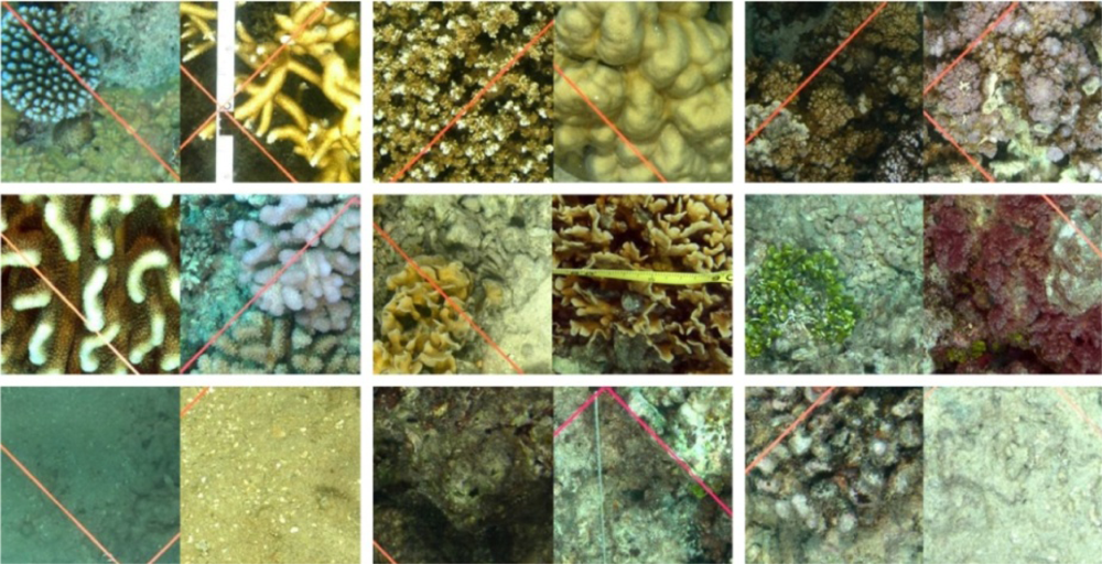
The relative performance of published classification algorithms has not been tested on common datasets. To address this issue, our proposed classification scheme and four other existing algorithms were tested against six image datasets that represent a variety of challenging environments. A seventh dataset is used along with datasets 1–3 to guide selection of the various options available in our proposed framework. Finally, an eighth dataset is used to illustrate the potential for generating thematic maps of large contiguous areas of the seabed using this automated classification framework. A brief summary of the image datasets used in this work is presented in Table 3. Appendix 2 contains a more detailed description of the various datasets. Figure 3 shows an example of images patches from the EILAT dataset.
4.3. Criteria for Evaluation and Comparison with Other Methods
An error matrix and precision recall curve are used to evaluate the classification quality of each classification method. The error matrix quantifies the accuracy of each classified category as a percentage based on the total number of validation points in each category [36]. The overall accuracy (OA) of the classified dataset is derived from the error matrix as the sum of the number of correctly classified tested examples divided by the total number of tested examples. The precision-recall curve is computed by varying the threshold on the classifier (from high to low) and plotting the values of precision against recall for each threshold value. The average precision (AP) summarizes the precision-recall curve by measuring the area under the curve.
To compare the proposed framework, four underwater image algorithms (Pizarro [8], Beijbom [4], Marcos [9] and Stokes and Deane [10]) and two state-of-the-art texture classification methods (Caputo [19] and Zhang [20]) are used. Each algorithm is implemented as closely as possible to the original papers (the parameters are tuned with exhaustive search). The first four algorithms (initially developed for underwater imagery) are used to classify all six of the test datasets. The two texture-classification algorithms are only used to classify the three texture datasets. The results for each algorithm are evaluated in terms of the overall accuracy and average precision of the classification. The time required to execute each method is reported in Section 5.3. The effect of changing the number of training samples in the datasets is also evaluated in Section 5.3.
4.4. Mosaic Image Classification
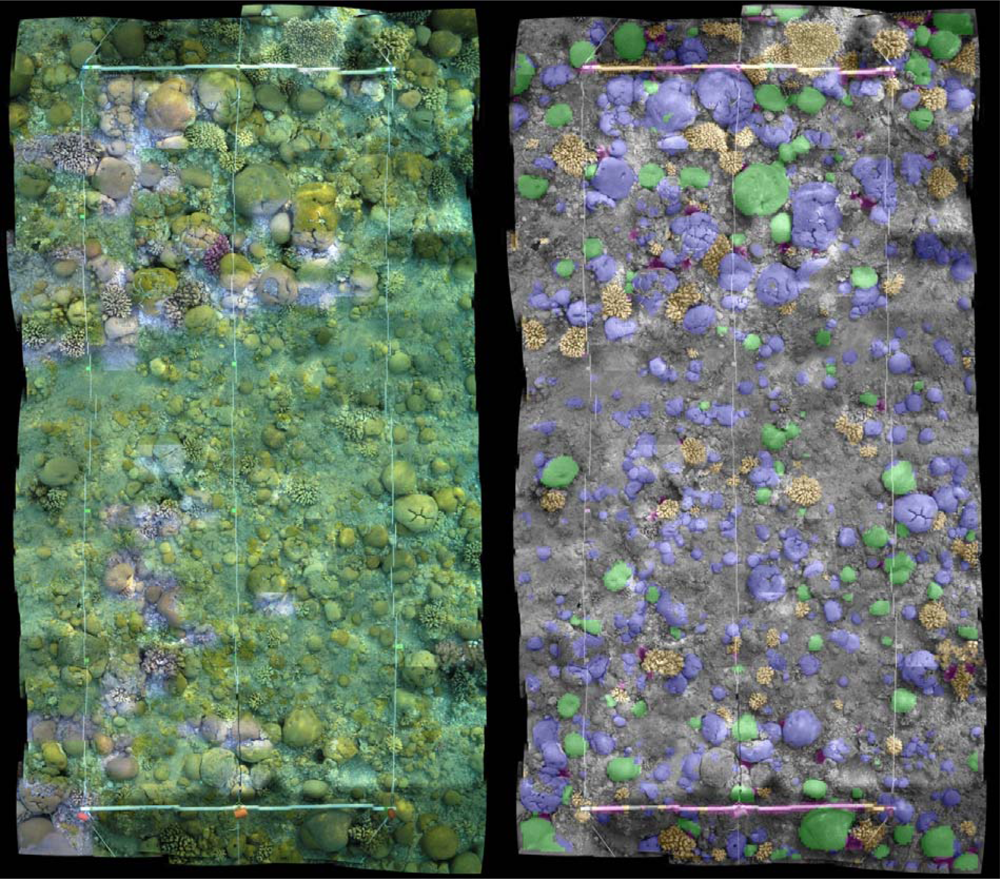
Finally, our proposed algorithm and first four algorithms are implemented on a mosaic image to create a thematic map of a contiguous section of the seabed covering an area larger than a single image. The mosaic is created using the methods by [32–34] from survey images (283 high-resolution digital still images and rendered at 1 mm per pixel) of shallow water coral reefs in the Red Sea, near Eilat [37]. The mosaic covers an area of 19.2 square meters.
To train the classifier for the mosaic, we use entire 1,123 image patches in the EILAT dataset. The sliding window used to classify the mosaic is of size 64 × 64 pixels (same as the size of training image patches). The sliding window is moved with 16 pixels shift (either horizontally or vertically) per iteration. In total 73,600 image patches are classified within the mosaic image.
To examine the effects of morphological filtering, we created a ground truth by manually classifying the Red Sea mosaic with help of experts. We use this ground truth for a qualitative assessment of the proposed method and the other existing algorithms. The classification results (color coded) on the mosaic are presented and discussed in the Section 5.4.
5. Results
Having presented, in the previous section, the criteria and methods for evaluating the classifiers, this section now presents experimental results. These results allow for assessing the impact of different configurations, for evaluating and validating the proposed method, for comparing against the other selected approaches and for making recommendations on the best configuration for future datasets.
5.1. Evaluation of Different Configurations
Among the image enhancement options, (step 1), CLAHS alone produced the best results for the EILAT, RSMAS and EILAT 2 datasets. CLAHS with color channel stretching produced the best results for the MLC 2008 dataset (Table 4). CLAHS, color correction and color channel stretching produced the best result for the MLC 2008 dataset.
Regarding the feature extraction options, (step 2), the combined feature vector of color histogram (hue and opponent angle), CLBP, Gabor filter response and GLCM worked most effectively on EILAT, RSMAS and MLC 2008 datasets (Table 5). For the EILAT 2 dataset, the color features are not discriminative enough to aid the classification performance in the combined feature vector. In general, if color images are available, color histograms can be used together with texture descriptors. The combination of CLBP, Gabor filter response and GLCM (texture descriptors) works better than any single feature in all four datasets.
With respect to the available kernel mapping options (step 3), the best results are obtained by using both the chi-square and Hellinger kernels along with L1 normalization, as illustrated in Table 6.
Finally, for the EILAT and RSMAS datasets the best classifier (step 4) and dimension reduction (step 6) options are the ones using the KNN classifier with dimension reduction by PCA and Fisher kernel mapping (Table 7). For the EILAT 2 dataset, the SVM classifier without dimension reduction produces the highest overall accuracy. For MLC 2008, dataset, the maximum overall accuracy is achieved with probability density weighted mean distance classifier (PDWMD) and no dimension reduction.
Using the experimental results above (Tables 4, 5, 6 and 7), we select the configurations shown in Table 8 for the respective datasets to be compared with other published methods. For texture datasets (Columbia-Utrecht Reflectance and Texture (CURET), Kungliga Tekniska Högskolan (KTH), University of Illinois at Urbana-Champaign (UIUC)), we use the same configuration as the EILAT dataset without color histograms as feature descriptors. The texture types, distribution and size of the grey texture datasets are similar to those of the EILAT dataset.
5.2. Evaluation of Proposed Classification Method
The proposed image classification method is evaluated using the MLC 2008 dataset by constructing a precision-recall curve and error matrix. Precision is defined as the fraction of retrieved instances that are relevant, while recall corresponds to the fraction of relevant instances that are retrieved. High recall indicates that an algorithm is capable of returning most of the relevant results. High precision indicates that an algorithm returns more relevant results than irrelevant. The precision-recall curves (Figure 4) and error matrix (Table 9) for our proposed method applied to the MLC 2008 dataset result in 85.3% overall accuracy and 75.3% average precision. The highest precision value is observed for Pocillopora, and the lowest for the macroalgae class, as shown in Figure 3.
Table 9 shows the error matrix of our method when applied on the MLC 2008 dataset. The highest number of examples in this dataset is from the crustose coralline algae (CCA) class, which also has frequent overlaps with other classes. The error matrix reflects this fact, as other classes are highly confused with CCA (as shown in the 2nd row of Table 9).
5.3. Comparison with Other Methods
Table 10 shows error matrices for all four of the compared classification methods when tested on the MLC 2008 dataset. The proposed framework achieves the highest overall accuracy (OA) and highest average precision for five datasets among six (Tables 11 and 12). For the EILAT dataset, all methods work reasonably well, though our method achieves the highest overall accuracy (96.9%). The second highest OA is achieved with the Marcos classification (87.9%). The results of the RSMAS dataset are similar to those of the EILAT dataset, except the second most accurate method is the Beijbom classification, with an overall accuracy of 85.4%. For the MLC 2008 dataset, our method results in 85.5% overall classification accuracy.
The proposed method achieves almost similar classification accuracy when tested against traditional and texture-only image datasets (Table 11). Most of the other methods, however, perform significantly worse against texture-only datasets. The failure of the methods by Marcos [9], Stokes & Deane [10], Pizarro [8] and Beijbom [4] on standard texture datasets indicates that these methods rely heavily on color information. Heavy reliance on color information may limit the robustness of classification algorithms, since color can be inconsistent or absent in underwater datasets.
The two state-of-the-art texture-classification algorithms (Caputo [19], Zhang [20]) perform well relative to the proposed method. For the UIUC dataset, our method attains 97.3% overall accuracy, but can not beat Zhang [20], which achieves 99% OA. The UIUC dataset has higher resolution than the other datasets; therefore, dense descriptors, such as our method, might be influenced by the background information resulting in inaccurate classification. Our method is mainly suitable for small patch sized image datasets, which is useful for classified mapping on mosaics.
For CURET and KTH datasets, which have a smaller patch size, our proposed method has higher overall accuracy than the texture-only method (Zhang [20]). We compare our proposed method with their method in the same experimental conditions and acquire 99.2% accuracy for the CURET dataset and 98.3% for KTH datasets, where the reported as state-of-the-art Caputo [19] obtains 98.6% accuracy for CURET dataset and Zhang [20] obtains 96.7% for the KTH dataset.
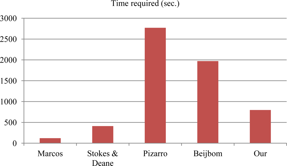
The classification methods by Marcos and Stokes & Deane are computationally efficient (Figure 5). Our method requires less time than the methods by Pizarro [4] and Beijbom [8]. For the method of Pizarro, the time for the generation of 500 visual word vocabulary is considered, which normally can be computed offline. If that time is taken out, this method can be considered as fast as our method. In this context, the method by Stokes and Deane can be considered very efficient. All these methods are implemented in Matlab 2010a and tested on Intel core i5-2430M CPU with 2.4 GHz speed and 6 GB RAM.
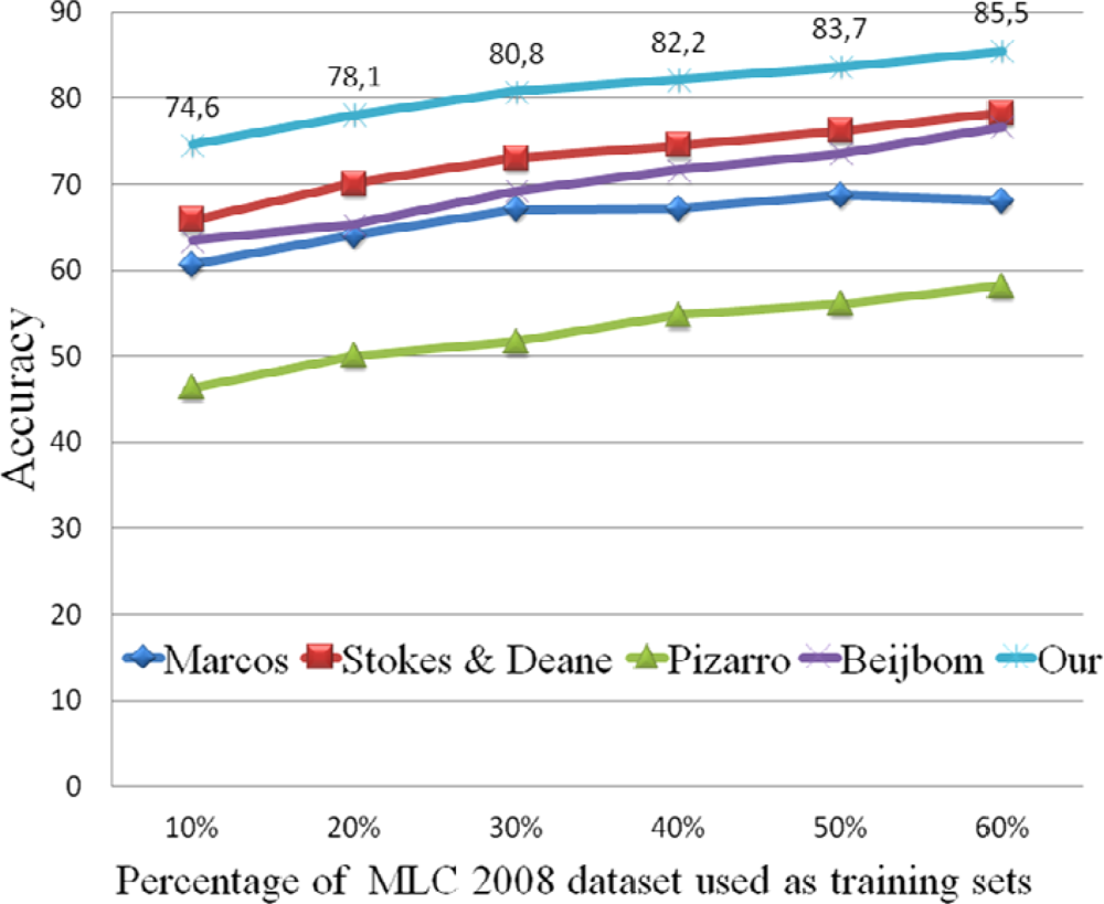
The performance consistency is tested as a function of the percentage of training samples used. As the percentage of the training samples for the MLC 2008 datasets changes from 10% to 60%, accuracy increases gradually in all the methods. This result reflects the fact that more training samples can produce stronger classifiers (Figure 6).
5.4. Classifying Image Mosaics
Applying the classification method to segment the full mosaic of Red Sea survey images takes approximately seven hours on an Intel core i5-2430M CPU with 2.4 GHz speed and 6 GB RAM. The image patches are of size 64 × 64 pixels with a sliding window of 16-pixels shift per iteration, result in 73,600 image patches to classify in the full mosaic.
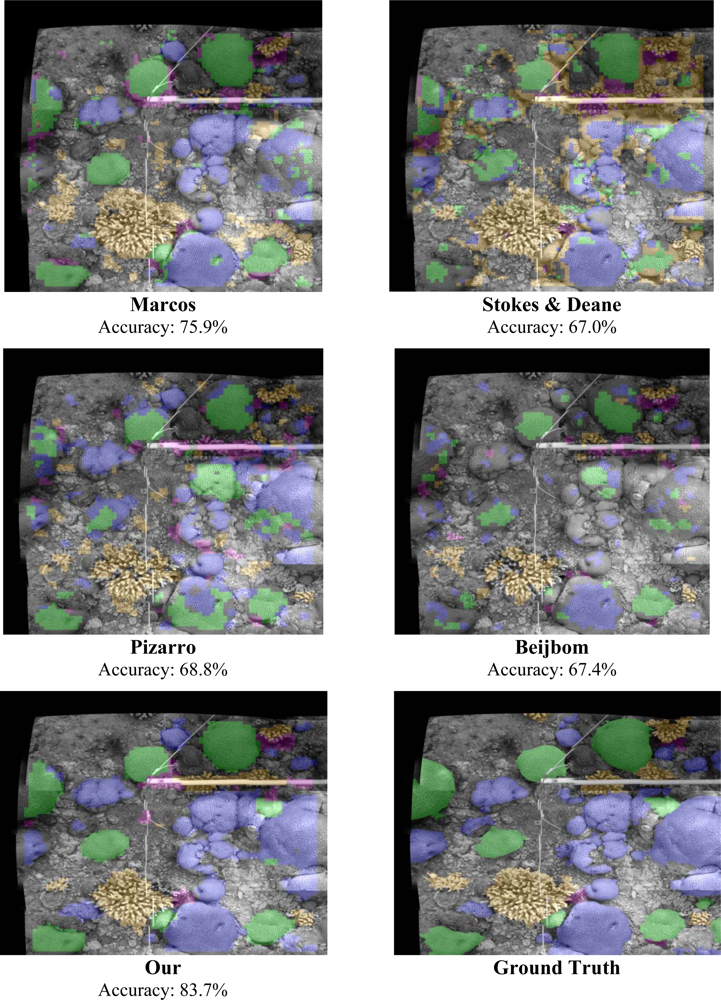
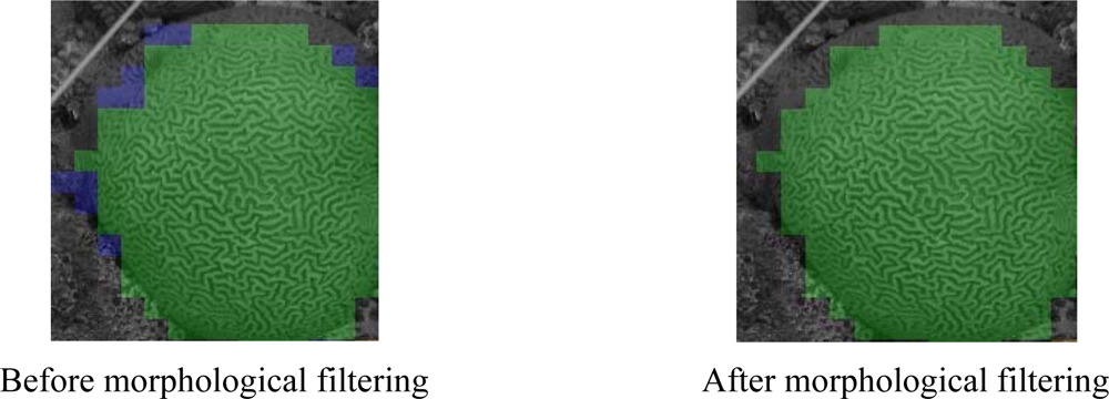
The classification results of each method on the Red Sea mosaic image are shown in Figure 7. Misclassifications tend to be on the borders of objects (Figure 8). Morphological filtering alters some results by maintaining neighborhood consistency (Figure 8, right). Morphological filtering increases the classification accuracy from 82.8% to 83.7% (Figure 8). In Figure 9, the left is the input mosaic image and on the right is the segmented and color coded thematic map.
5.5. Recommendations for Classifying Future Datasets
The application of multiple classification methods to six image datasets results in the following recommendations concerning future image classifications.
- If the dataset contains low contrast or blurred images, CLAHS works very well as an image enhancement step. If color markers are available in raw images, color correction can be performed to enhance the color constancy.
- For texture description, the concatenation of GLCM, Gabor filter response and CLBP works consistently well. If images have good reliable color information, then opponent angle and hue color channel histograms can be added, with the texture descriptor assigning equal weights to both color and texture descriptors.
- In all the cases of image patch classification, sparsely populated bins within histograms possess higher distinctive information than the high frequency bins. This statement is based on the assumption that high frequency bins often represent the background of the object and contain less distinctive information. The chi-square and Hellinger kernels can be used to modify bin counts and boost the population of low frequent bins. L1 normalization of the feature vector is necessary in all cases before applying the classifier for training and testing.
- If the dataset is small (datasets with training samples less than 5,000 are considered as small ones), then PCA and Fisher kernel mapping works very effectively to reduce the feature dimension. However, for large (Datasets with training samples more than 12,000 are considered as large ones) datasets, almost all the features become useful, and the dimension reduction is much less effective. In large datasets, almost all the dimensions become discriminative, and only a few dimensions are reduced with PCA. Therefore, for large datasets, this dimension reduction step can be avoided.
- Class frequency works well as prior in all the cases.
- For smaller datasets, the KNN classifier has the best performance. However, as the datasets get larger, the effectiveness of this method reduces, owing to the higher storage requirements, lower efficiency in classification response and lower noise tolerance. Some recent works [38] address this problem of KNN. However, SVM (linear SVM with one against the rest scheme) and neural networks (multilayer perception with back projection configuration) can be appropriate classifiers for bigger datasets. For underwater images, the classification based on probability density weighted mean distance (PDWMD) from the tail of the distribution by Stokes and Deane [10] works efficiently, both in terms of time and efficiency.
- Morphological filtering can increase the accuracy of the classification results.
- For smaller datasets, the KNN classifier has the best performance. However, as the datasets get larger, the effectiveness of this method reduces because of high storage requirements, low efficiency in classification response and low noise tolerance. Some recent works [38] address this problem of KNN. However, SVM (linear SVM with one against the rest scheme) and neural networks (multilayer perception with back projection configuration) can be appropriate classifiers for bigger datasets. For underwater images, the classification based on probability density weighted mean distance (PDWMD) from the tail of the distribution [10] works efficiently both in terms of time and efficiency.
- In our method, all the features used are partially or completely scale and rotation invariant. These features are therefore able to mitigate the effects of limited scale variation of individual classes. For larger scale variation, it is important to have enough training examples of individual classes at different scales. In the future, multi-resolution mapping might be useful for benthic habitat covering large scale variations of individual classes.
6. Conclusion
Large datasets of benthic images, which have been enabled by digital acquisition and innovative platforms, such as remotely operated vehicles (ROVs) or autonomous underwater vehicles (AUVs), provide a new opportunity for remote sensing of coral reefs, as well as a challenge. The opportunity lies in the types of measurements that can be made from direct remote sensing of benthic organisms. The challenge lies in efficiently extracting biological or ecological information from the raw images. Some form of automated analysis will be required to make full use of this rich data source.
Our proposed method presents a novel image classification scheme for benthic coral reef images that achieved the highest overall classification accuracy of any of the tested methods and had moderate execution times. This paper used six standard datasets to compare the set of methods that are representative of the state-of-the-art in automated classification of seabed images. On state of the art Moorea labeled corals (MLC) dataset [4], our method achieved 85.5% overall accuracy, whereas all the other compared methods attained less than 80%, including the method by Beijbom [4].
The proposed method can be configured to the characteristics (e.g., size, number of classes and resolution of the samples, color information availability, class types and so forth) of individual datasets. We provided guidelines for choosing the appropriate configuration for future classification of reef images. The results suggest that using a selective combination of various preprocessing steps, feature extraction methods, kernel mappings, priori and classifiers for various datasets can give better results than using a single method for all datasets. The results can be extended over large continuous areas by using mosaics of underwater images. On the Red Sea mosaic image, our proposed method resulted in 83.7% overall accuracy, which is at least 8% higher than the other methods tested.
The experimental part of our work allowed us to identify classification problems that are specific to underwater images. On one hand, there are many classes in underwater imagery that have samples with very clear differences in shape, color, texture, size, rotation, illumination, view angle, camera distance and light conditions. On the other hand, there are overlapping classes that look almost the same from specific angles and distances. Finding optimal patch size and patch shift are still open questions. Moreover, additional challenges, such as motion blurring, color attenuation, refracted sunlight patterns, water temperature variation, sky color variation and scattering effects, have to be reduced to maintain the image quality and the reliable information content. These issues highlight areas where future research may continue to improve the accuracy and efficiency of automated classification methods.
Applying automated classification techniques to mosaic composites produces a rapid (in terms of expert annotation time) technique of characterizing reef communities that can be used to track changes over time. Quantifying benthic community composition over the scale of hundreds of square meters by automated analysis of underwater image mosaics is a novel capability in coral reef science and provides a new spatial scale from which reef dynamics can be observed and studied. In addition to the time saved by applying a single training dataset to a large-area reef mosaic, applying automated classification schemes to mosaics can also reduce computational time, since it bypasses the redundancy of classifying highly overlapping images. Furthermore, the techniques presented here are not uniquely limited to coral reef classification and may prove useful in other ecosystems.
Acknowledgments
This work was partially funded by the Spanish MICINN under grant CTM2010-15216 (MuMap) and by the EU Project FP7-ICT-2011-288704 (MORPH) and US DoD/DoE/EPA project ESTCP SI2010. ASM Shihavuddin was supported by the MICINN under the FI program. Art Gleason was supported by a grant from the Gale Foundation. The authors would like to acknowledge Assaf Zvuloni and Yossi Loya of the Tel Aviv University for the use of the Red Sea survey imagery. We would like to thank the reviewers and the editors for their invaluable comments, which have helped us to significantly improve the manuscript. We would also like to thank Kasey Cantwell and R. Pamela Reid’s group at the University of Miami for help on the creation of the EILAT and RSMAS datasets, Oscar Beijbom for making his implementation publicly available on the web and also the authors of Weka, CLBP, Prtools and Vlfeat toolboxes.
References
- Turner, W.; Spector, S.; Gardiner, N.; Fladeland, M.; Sterling, E.; Steininger, M. Remote sensing for biodiversity science and conservation. Trends Ecol. Evol 2003, 18, 306–314. [Google Scholar]
- Kohler, K.E.; Gill, S.M. Coral Point Count with Excel extensions (CPCe): A Visual Basic program for the determination of coral and substrate coverage using random point count methodology. Comput. Geosci 2006, 32, 1259–1269. [Google Scholar]
- Pican, N.; Trucco, E.; Ross, M.; Lane, D.; Petillot, Y.; Tena Ruiz, I. Texture Analysis for Seabed Classification: Co-Occurrence Matrices vs. Self-Organizing Maps. Proceedings of OCEANS ’98, Nice, France, 28 September–01 October 1998; 1, pp. 424–428.
- Beijbom, O.; Edmunds, P.J.; Kline, D.I.; Mitchell, B.G.; Kriegman, D. Automated Annotation of Coral Reef Survey Images. Proceedings of IEEE Conference on Computer Vision and Pattern Recognition (CVPR), Providence, Rhode Island, 16–21 June 2012.
- Gracias, N.; Negahdaripour, S.; Neumann, L.; Prados, R.; Garcia, R. A motion compensated filtering approach to remove sunlight flicker in shallow water images. Oceans 2008, 2008, 1–7. [Google Scholar]
- Schechner, Y.Y.; Karpel, N. Attenuating Natural Flicker Patterns. Proceedings of IEEE/MTS OCEANS 04 Conference, Kobe, Japan, 9–12 November 2004.
- Shihavuddin, A.S.M.; Gracias, N.; Garcia, R. Online Sunflicker Removal using Dynamic Texture Prediction. Proceedings of International Joint Conference on Computer Vision, Imaging and Computer Graphics Theory and Applications, Rome, Italy, 24–26 February, 2012; pp. 161–167.
- Pizarro, O.; Rigby, P.; Johnson-Roberson, M.; Williams, S.; Colquhoun, J. Towards Image-Based Marine Habitat Classification. Proceedings of OCEANS 08, Quebec City, QC, Canada, 15–18 September 2008.
- Marcos, M.; Shiela, A.; David, L.; Peñaflor, E.; Ticzon, V.; Soriano, M. Automated benthic counting of living and non-living components in Ngedarrak Reef, Palau via subsurface underwater video. Environ. Monit. Assess 2008, 145, 177–184. [Google Scholar]
- Stokes, M.D.; Deane, G.B. Automated processing of coral reef benthic images. Limnol. Oceanogr. Methods 2009, 7, 157–168. [Google Scholar]
- Padmavathi, G.; Muthukumar, M.; Thakur, S. Kernel Principal Component Analysis Feature Detection and Classification for Underwater Images. Proceedings of 3rd International Congress on Image and Signal Processing (CISP), Yantai, China, 16–18 October 2010; 2, pp. 983–988.
- Marcos, M.; Angeli, S.; David, L.; Peaflor, E.; Ticzon, V.; Soriano, M. Automated benthic counting of living and non-living components in Ngedarrak Reef, Palau via subsurface underwater video. Environ. Monit. Assess 2008, 145, 177–184. [Google Scholar]
- Mehta, A.; Ribeiro, E.; Gilner, J.; van Woesik, R. Coral Reef Texture Classification using Support Vector Machines. Proceedings of International Joint Conference on Computer Vision, Imaging and Computer Graphics Theory and Applications (VISAPP), Barcelona, Spain, 8–11 March 2007; pp. 302–310.
- Gleason, A.; Reid, R.; Voss, K. Automated Classification of Underwater Multispectral Imagery for Coral Reef Monitoring. Proceedings of OCEANS 07, Miami, FL, USA, 29 September–4 October 2007; pp. 1–8.
- Johnson-Roberson, M.; Kumar, S.; Willams, S. Segmentation and Classification of Coral for Oceanographic Surveys: A Semi-Supervised Machine Learning Approach. Proceedings of OCEANS 2006, Asia Pacific, Singapore, 16–19 May 2007.
- Johnson-Roberson, M.; Kumar, S.; Pizarro, O.; Willams, S. Stereoscopic Imaging for Coral Segmentation and Classification. Proceedings of OCEANS 06, Singapore, 18–21 September 2006; pp. 1–6.
- Clement, R.; Dunbabin, M.; Wyeth, G. Toward Robust Image Detection of Crown-of-thorns Starfish for Autonomous Population Monitoring. In Australasian Conference on Robotics & Automation; Sammut, C., Ed.; Australian Robotics and Automation Association Inc.: Sydney, Australia, 2005. [Google Scholar]
- Soriano, M.; Marcos, S.; Saloma, C.; Quibilan, M.; Alino, P. Image Classification of Coral Reef Components from Underwater Color Video. Proceedings of 2001 MTS/IEEE Conference and Exhibition OCEANS, Honolulu, HI, USA, 5–8 November 2001; 2, pp. 1008–1013.
- Caputo, B.; Hayman, E.; Fritz, M.; Eklundh, J.O. Classifying materials in the real world. Image Vis. Comput 2010, 28, 150–163. [Google Scholar]
- Zhang, J.; Lazebnik, S.; Schmid, C. Local features and kernels for classification of texture and object categories: A comprehensive study. Int. J. Comput. Vis 2007, 73, 213–238. [Google Scholar]
- Zuiderveld, K. Contrast Limited Adaptive Histogram Equalization. Graphics GEMs IV; Academic Press Professional, Inc.: San Diego, CA, USA, 1994; pp. 474–485. [Google Scholar]
- Finlayson, G.D.; Schiele, B.; Crowley, J.L. Comprehensive Colour Image Normalization. Proceedings of ECCV'98 Fifth European Conference on Computer Vision, Freiburg, Germany, 2–6 June 1998; 1406, pp. 475–490.
- Gehler, P.; Nowozin, S. On Feature Combination for Multiclass Object Classification. Proceedings of IEEE 12th International Conference on Computer Vision (ICCV), Kyoto, Japan, 29 September–2 October 2009; pp. 221–228.
- Haley, G.; Manjunath, B. Rotation-invariant texture classification using a complete space-frequency model. IEEE Trans. Image Process 1999, 8, 255–269. [Google Scholar]
- Haralick, R.M.; Shanmugam, K.; Dinstein, I. Textural features for image classification. IEEE Trans. Syst. Man Cybern. 1973, SMC-3, 610–621. [Google Scholar]
- Soh, L.; Tsatsoulis, C. Texture analysis of SAR sea ice imagery using gray level co-occurrence matrices. IEEE Trans. Geosci. Remote Sens 1999, 37, 780–795. [Google Scholar]
- Clausi, D.A. An analysis of co-occurrence texture statistics as a function of grey level quantization. Can. J. Remote Sens 2002, 28, 45–62. [Google Scholar]
- Guo, Z.; Zhang, L.; Zhang, D. A completed modeling of local binary pattern operator for texture classification. IEEE Trans. Pattern Anal. Mach. Intell 2010, 19, 1657–1663. [Google Scholar]
- Van de Weijer, J.; Schmid, C. Coloring Local Feature Extraction. Proceedings of the 9th European Conference on Computer Vision ECCV’06, Graz, Austria, 7–13 May 2006; pp. 334–348.
- Mika, S.; Ratsch, G.; Weston, J.; Scholkopf, B.; Mullers, K. Fisher Discriminant Analysis with Kernels. Proceedings of the 1999 IEEE Signal Processing Society Workshop, Neural Networks for Signal Processing IX, 1999, Berlin, Germany, 25 August 1999; pp. 41–48.
- Ruderman, D.L. The statistics of natural images. Netw. Comput. Nat. Syst 1994, 4, 517–548. [Google Scholar]
- Lirman, D.; Gracias, N.; Gintert, B.; Gleason, A.C.R.; Deangelo, G.; Gonzalez, M.; Martinez, E.; Reid, R.P. Damage and Recovery Assessment of Vessel Grounding Injuries on Coral Reef Habitats Using Georeferenced Landscape Video Mosaics. Limnol. Oceanogr.: Methods 2010, 8, 88–97. [Google Scholar]
- Escartin, J.; Garcia, R.; Delaunoy, O.; Ferrer, J.; Gracias, N.; Elibol, A.; Cufi, X.; Neumann, L.; Fornari, D.J.; Humphris, S.E. Globally aligned photomosaic of the Lucky Strike hydrothermal vent field (Mid-Atlantic Ridge, 37°18.5′N): Release of georeferenced data, mosaic construction, and viewing software. Geochem. Geophys. Geosyst. 2008, 9. [Google Scholar] [CrossRef]
- Lirman, D.; Gracias, N.; Gintert, B.; Gleason, A.; Reid, P.; Negahdaripour, S.; Kramer, P. Development and application of a video-mosaic survey technology to document the status of coral reef communities. Environ. Monit. Assess 2007, 125, 59–73. [Google Scholar]
- Kohavi, R. A. Study of Cross-Validation and Bootstrap for Accuracy Estimation and Model Selection. Proceedings of the Fourteenth International Joint Conference on Artificial Intelligence, IJCAI 95, Montréal, QC, Canada, 20–25 August 1995; pp. 1137–1143.
- Congalton, R.G.; Green, K. Assessing the Accuracy of Remotely Sensed Data; Lewis Publishers: Boca Raton, FL, USA, 1999; p. 137. [Google Scholar]
- Loya, Y. The Coral Reefs of Eilat; Past, Present and Future: Three Decades of Coral Community Structure Studies. In Coral Reef Health and Disease; Springer-Verlag: Berlin/Heidelberg, Germany, 2004; pp. 1–34. [Google Scholar]
- Garcia, S.; Derrac, J.; Cano, J.; Herrera, F. Prototype Selection for Nearest Neighbor Classification: Taxonomy and Empirical Study. IEEE Trans. Pattern Anal. Mach. Intell 2012, 34, 417–435. [Google Scholar]
Appendix 1

Table A1.
List of statistics used for GLCM feature calculations. The GLCM feature vector consisted of 22 features calculated from the following table. C is the L1 normalized co-occurrence matrix (defined over an image to be the distribution of co-occurring values at a given offset). The pixel row and column are represented by i and j. N is the number of distinct gray levels in a quantized image (we used 16 in our case), μ and S are the mean and standard deviation and H is the entropy of C. C is a N by N matrix. I is the input image of n × m size. The offset is [Δx Δy]. We used [0 3], [−3 3], [−3 0], [−3 −3] offset values; calculated statistics individually for each features and then averaged to get final results. These offset values represent 0, 45, 90 and 135 degrees angular neighborhood with a distance of three pixels from the center pixel.Co-occurrence matrix,
Normalized Co-occurrence matrix,
| Co-occurrence indicator used in the features | |
|---|---|
| Statistics | Formulas | |
|---|---|---|
| 1 | Maximum Probability [33] | |
| 2 | Uniformity [12,33] | |
| 3 | Entropy [33] | |
| 4 | Dissimilarity [33] | |
| 5 | Contrast [12,33] | |
| 6 | Inverse Difference [33] | |
| 7 | Inverse Difference moment [33] | |
| 8 | Correlation 1 [12,33] | |
| 9 | Inverse Difference Normalized [27] | |
| 10 | Inverse Difference Moment Normalized [27] | |
| 11 | Sum of Squares: Variance [12] | |
| 12 | Sum Average [12] | |
| 13 | Sum Entropy [12] | |
| 14 | Sum Variance [12] | |
| 15 | Difference Variance [12] | |
| 16 | Difference Entropy [12] | |
| 17 | Info. measure of correlation 1 [12] | |
| 18 | Info. measure of correlation 2 [12] | |
| 19 | Autocorrelation [33] | |
| 20 | Correlation 2 [12,33] | |
| 21 | Cluster Shade [33] | |
| 22 | Cluster Prominence [33] |
Appendix 2
A2.1. EILAT Dataset
The EILAT dataset contains 1,123 image patches, each being 64 × 64 pixels in size (Figure 3), taken from images of reef survey near Eilat in the Red sea. A group of experts have visually classified the images into eight classes (sand, urchin, branches type I, brain coral, favid coral, branches type II, dead coral and branches type III). Two of the classes have a larger number of examples compared with others. The image patches were extracted from the original, full-size images, which were all taken with the same camera.
A2.2. RSMAS Dataset
The RSMAS dataset was obtained from reef survey images collected by divers from the Rosenstiel School of Marine and Atmospheric Sciences of the University of Miami. This dataset has examples of different classes of underwater coral reefs taken with different cameras at different times and places. The database consists of 766 image patches; each 256 × 256 pixels in size, of 14 different classes (see Figure A1). The image patches are larger than those in the EILAT dataset, which means that they are more likely to contain mixed classes.
Figure A1.
A subset of the RSMAS dataset; showing 12 examples, in columns, of each of the 14 classes (in rows from top to bottom: Acropora cervicornis (ACER), Acropora palmata (APAL), Colpophyllia natans (CNAT), Diadema antillarum (DANT), Diploria strigosa (DSTR), Gorgonians (GORG), Millepora alcicornis (MALC), Montastraea cavernosa (MCAV), Meandrina meandrites (MMEA), Montipora spp. (MONT), Palythoas palythoa (PALY), Sponge fungus (SPO), Siderastrea siderea (SSID) and tunicates (TUNI).

A2.3. Moorea-Labeled Corals (MLC) dataset
The MLC dataset [4] is a subset of images collected for the Moorea Coral Reef Long Term Ecological Research site (MCR-LTER) packaged for computer vision research. It contains 2,055 images from three habitats: fringing reef, outer 10 m and outer 17 m, from 2008, 2009 and 2010. It also contains random points that have been annotated. The nine most abundant labels include four non-coral classes: (1) crustose coralline algae (CCA), (2) turf algae (Turf), (3) macroalgae (Macro) and (4) sand; and five coral genera: (5) Acropora (Acrop), (6) Pavona (Pavon), (7) Montipora (Monti), (8) Pocillopora (Pocill) and (9) Porites (Porit). For our work, we are only using the 2008 dataset. In the MLC 2008 dataset, we used randomly selected 18,872 image patches, of 312 × 312 pixels in size, centered on the annotated points. All nine classes were represented in the random image patches (Figure A2).
Figure A2.
A subset of the MLC dataset showing two examples for each class. First row: Acropora, Porites, Montipora. Second row: Pocillopora, Pavona, Macroalgae. Third row: Sand, Turf algae, CCA.
Figure A2.
A subset of the MLC dataset showing two examples for each class. First row: Acropora, Porites, Montipora. Second row: Pocillopora, Pavona, Macroalgae. Third row: Sand, Turf algae, CCA.
The MLC is a good test dataset for classification algorithms, due to the large number of samples. Furthermore, each image contains plaques with known reference colors, thereby allowing accurate color correction. The MLC dataset is also challenging to classify, because each class exhibits great variability with respect to coral shape, color, scale and viewing angle. For example, two growth forms of Acropora and Porites have distinctly different appearance (Figure A2, top row left and center). The color and scale of the Pocillopora patches varies widely (Figure A2, middle row left). Macroalgae varies tremendously in shape and color and often protrudes from underneath the corals, resulting in image patches with mixed classes (Figure A2, middle row right). Both CCA and Turf algae tend to overgrow dead coral, which poses a challenge for automated analysis, since the coral skeleton retains its shape, but has the surface color and texture of the algae that overgrows it. Also, CCA and Turf are similar and, therefore, hard to discriminate.
A2.4. UIUCtex Dataset
The University of Illinois at Urbana-Champaign texture (UIUCtex) dataset [A1] contains 40 images in each of 25 texture classes: bark I, bark II, bark III, wood I, wood II, wood III, water, granite, marble, stone I, stone II, gravel, wall, brick I, brick II, glass I, glass II, carpet I, carpet II, fabric I, paper, fur, fabric II, fabric III and fabric IV (Figure A3). Textures were viewed under significant scale and viewpoint changes. The dataset includes non-rigid deformations, illumination changes and viewpoint-dependent appearance variations. All the image patches of this dataset are of 640 × 480 pixel size.
A2.5. CURET Texture Dataset
The Columbia-Utrecht Reflectance and Texture (CURET) dataset [A2] contains 61 texture classes, each with 92 images of size 200 × 200 pixels. Materials were imaged over varying pose and illumination, but at constant viewing distance. The changes of viewpoint and of the illumination direction significantly affect the texture appearance (Figure A4).
Figure A3.
A subset of UIUCtex dataset showing 4 examples from each of 5 classes (from the left group of 4 to the right: bark I, bark II, bark III, wood I and wood II).
Figure A3.
A subset of UIUCtex dataset showing 4 examples from each of 5 classes (from the left group of 4 to the right: bark I, bark II, bark III, wood I and wood II).
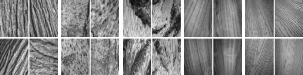
Figure A4.
A subset of CURET texture dataset showing 4 examples from each of three classes (from the left group of four to the right: felt, plaster and Styrofoam). Note the large intra-class variability caused by viewpoint and illumination changes.
Figure A4.
A subset of CURET texture dataset showing 4 examples from each of three classes (from the left group of four to the right: felt, plaster and Styrofoam). Note the large intra-class variability caused by viewpoint and illumination changes.

A2.6. KTH-TIPS Dataset
The Kungliga Tekniska Högskolan Textures under varying Illumination, Pose and Scale (KTH-TIPS) dataset [A3] contains images of 10 types of natural materials to provide variations in scale, as well as variations in pose and illumination. Images are captured at nine scales spanning two octaves (relative scale changes from 0.5 to two), viewed under three different illumination directions and three different poses, thus giving a total of nine images per scale and 81 images per material of the size 200 × 200 pixels. In total, there are 810 images comprising 10 different classes (sandpaper, crumpled aluminums foil, Styrofoam, sponge, corduroy, linen, cotton, brown bread orange peel, cracker B) present in this dataset (Figure A5).
A2.7. EILAT 2 Dataset
The EILAT 2 dataset contains 303 image patches. A group of experts have visually classified the images into five classes: sand, urchin, branching coral, brain coral and favid coral (Figure A6). Patches are of medium resolution (each 128 × 128 pixels in size) taken from points on the object to keep the visual aspects of the object and, in some cases, a portion of the background. Here, all the images are taken with the same camera. This dataset was used only as part of the process for selecting, which options to use in the image framework. Thus, the EILAT 2 dataset can be considered a middle ground between the EILAT and RSMAS datasets.
Figure A5.
A subset of KTH-TIPS dataset showing six examples from each of two classes: sponge (left) and cotton (right). The six examples include two different illuminations and three different scales.
Figure A5.
A subset of KTH-TIPS dataset showing six examples from each of two classes: sponge (left) and cotton (right). The six examples include two different illuminations and three different scales.
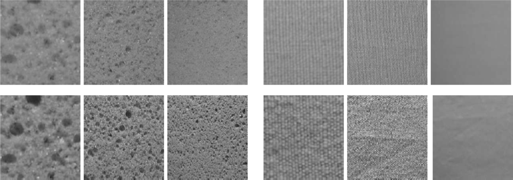
Figure A6.
A subset of the EILAT 2 dataset showing 10 examples, in columns, of each of the five classes (in rows from top to bottom: favid coral, brain coral, branching coral, sand and urchin).
Figure A6.
A subset of the EILAT 2 dataset showing 10 examples, in columns, of each of the five classes (in rows from top to bottom: favid coral, brain coral, branching coral, sand and urchin).

References
- Lazebnik, S.; Schmid, C.; Ponce, J. A sparse texture representation using local affine regions. IEEE Trans. Pattern Anal. Mach. Intell 2005, 27, 1265–1278. [Google Scholar]
- Dana, K.J.; van Ginneken, B.; Nayar, S.K.; Koenderink, J.J. Reflectance and texture of real-world surfaces. ACM Trans. Graph 1999, 18, 1–34. [Google Scholar]
- Hayman, E.; Caputo, B.; Fritz, M.; Eklundh, J.O. On the significance of real-world conditions for material classification. Eur. Conf. Comput. Vis 2004, 3024, 253–266. [Google Scholar]
Figure 1.
The proposed classification framework. For each of the seven steps, several options, or sub-steps, are available. The choices of which to use in each step depend on the characteristics of the dataset to classify. The steps themselves are described in Section 3, and guidance on how to choose among the options is given in Section 5. In the figure, the sub-steps colored in light blue are mandatory for all datasets. The light green colored sub-steps are optional. Grey colored sub-steps are mutually exclusive; meaning a single one in each step must be selected.
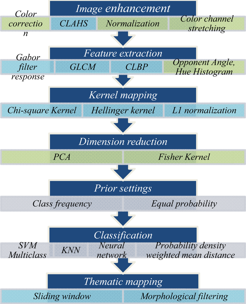
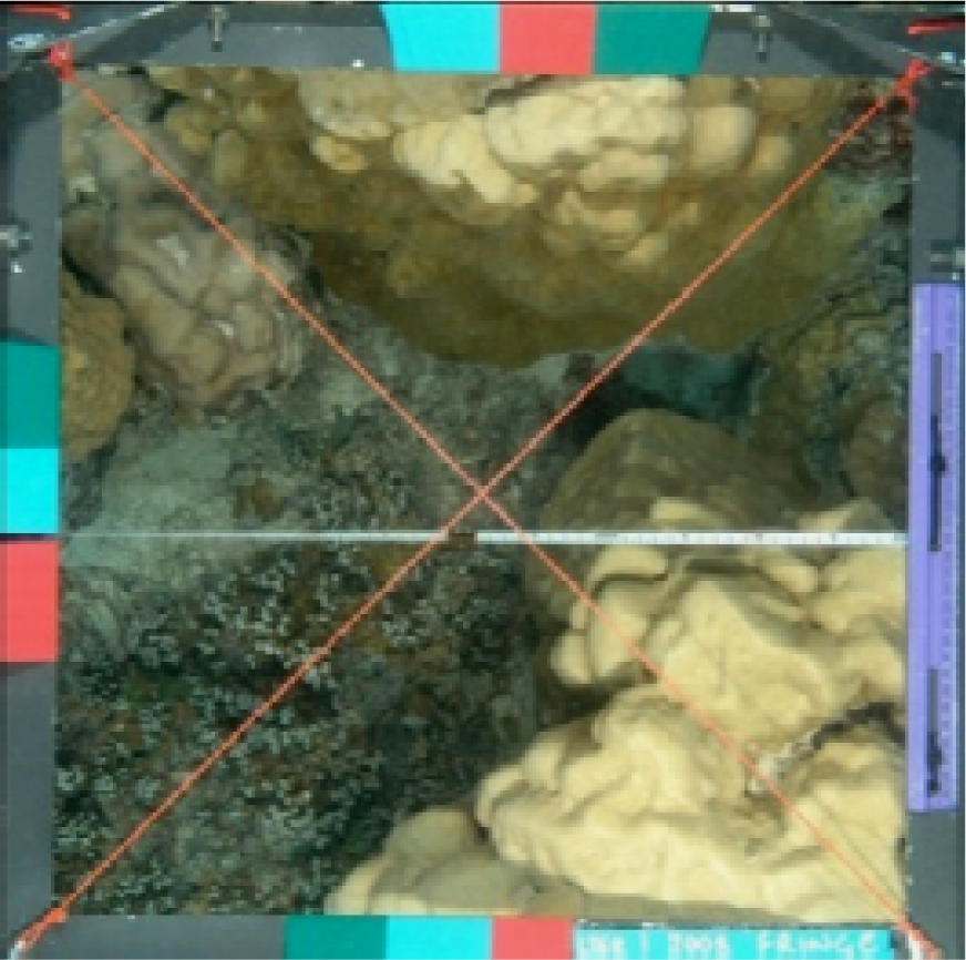
Figure 2.
Illustration of the presence of color markers in a raw image in the Moorea Coral Reef (MCR) dataset. There are three sets of color markers in this image. We only used one set on the top middle (comprising a three-color reference) to calculate the correction factors.
Figure 2.
Illustration of the presence of color markers in a raw image in the Moorea Coral Reef (MCR) dataset. There are three sets of color markers in this image. We only used one set on the top middle (comprising a three-color reference) to calculate the correction factors.

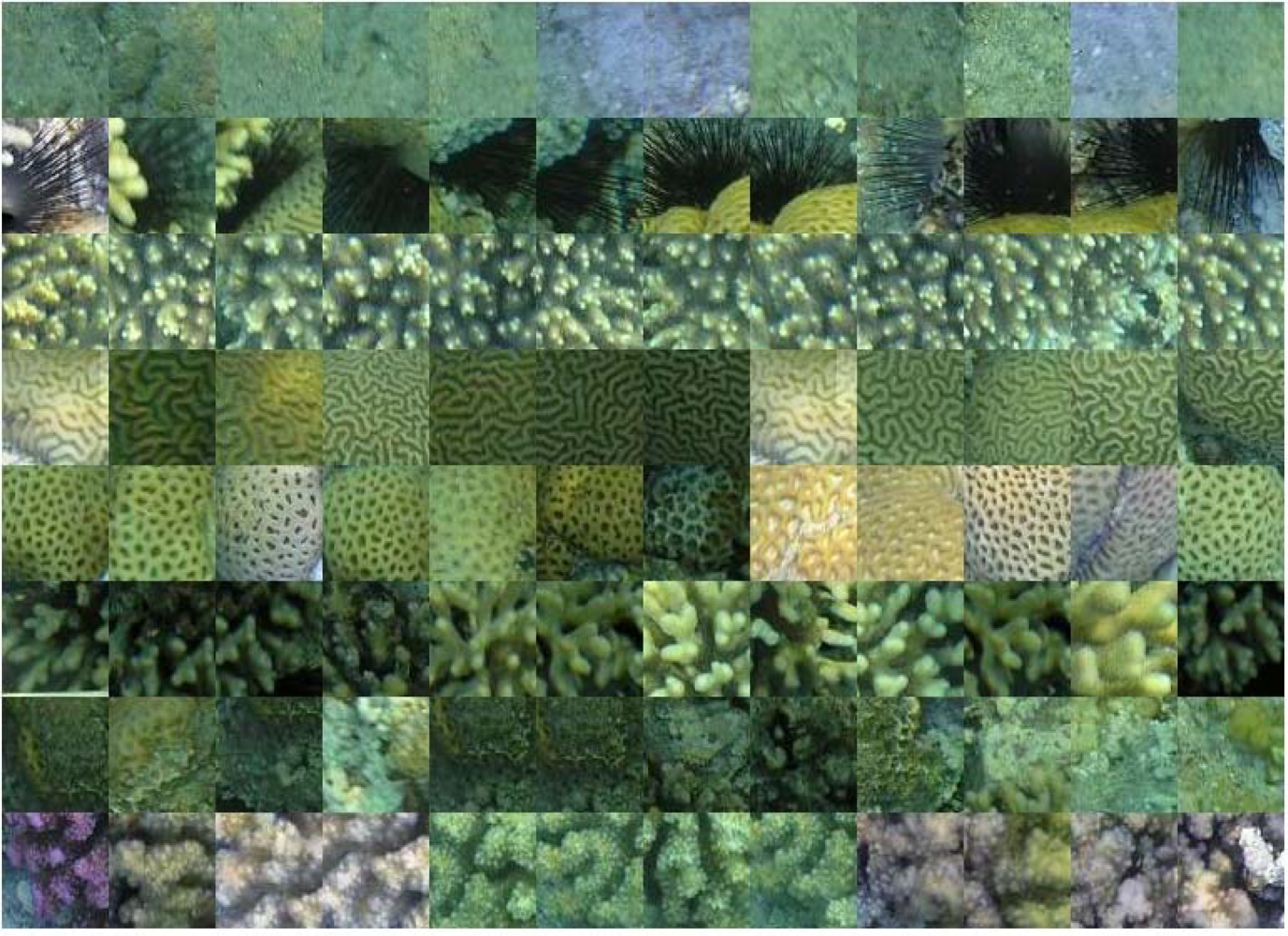
Figure 3.
Example images patches from the EILAT dataset showing 12 examples (in columns) of each of the eight classes (in rows, from top to bottom: sand, urchin, branches type I, brain coral, favid coral, branches type II, dead coral and branches type III).
Figure 3.
Example images patches from the EILAT dataset showing 12 examples (in columns) of each of the eight classes (in rows, from top to bottom: sand, urchin, branches type I, brain coral, favid coral, branches type II, dead coral and branches type III).

Figure 4.
Precision-recall curve for individual classes of the MLC 2008 dataset using our method. Average precision for this dataset was 75.3%. The highest precision was observed for Pocillopora, and the lowest value was for the macroalgae class. Our method resulted in 85.5% overall accuracy. In the MLC 2008 dataset, the highest number of examples was from the CCA class, which also had frequent overlaps with other classes.
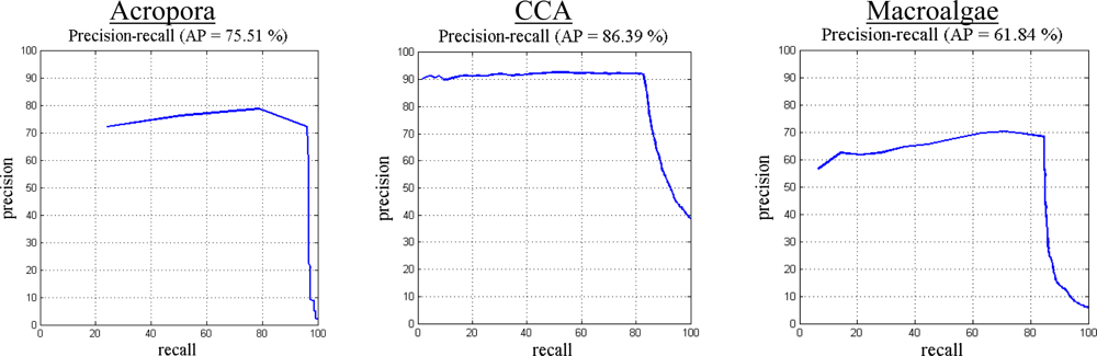
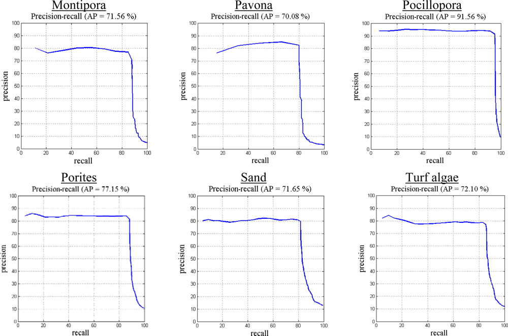
Figure 5.
The time required to classify the RSMAS dataset using four test methods.

Figure 6.
The overall accuracy of each method as a function of the number of images in the training data. This test is done on MLC 2008 dataset.
Figure 6.
The overall accuracy of each method as a function of the number of images in the training data. This test is done on MLC 2008 dataset.

Figure 7.
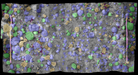
The accuracy of the tested classification methods applied to the Red Sea mosaic. The segmented images are color coded as: favid in violet, brain coral in green, branches I, II and III in orange, urchin in pink, dead corals and pavements are in grey.
Figure 7.
The accuracy of the tested classification methods applied to the Red Sea mosaic. The segmented images are color coded as: favid in violet, brain coral in green, branches I, II and III in orange, urchin in pink, dead corals and pavements are in grey.

Figure 8.
Effects of morphological filtering on classification results. (Left) The violets are misclassifications, which are removed after morphological filtering (right).
Figure 8.
Effects of morphological filtering on classification results. (Left) The violets are misclassifications, which are removed after morphological filtering (right).

Figure 9.
The original (left) and classified Red Sea mosaic (right). The segmented images are color coded with the same classification scheme as Figure 6.
Figure 9.
The original (left) and classified Red Sea mosaic (right). The segmented images are color coded with the same classification scheme as Figure 6.

Table 1.
A brief summary of methods classifying benthic images. All the methods mentioned here are specific to coral reef habitat classification. The methods in bold are used in Sections 5 for performance comparison and are referred to by the underlined author’s names. The last column, N, contains the number of classes used for testing in each method, as reported in their respective papers.
| Authors | Features | Classifiers | N |
|---|---|---|---|
| Beijbom [4] | Maximum response (MR) filter bank | Library for support vector machines (LIBSVM) | 9 |
| Padmavathi [11] | Bag of words using scale-invariant feature transform (SIFT) and kernel principal component analysis (KPCA) | Probabilistic neural network (PNN) | 3 |
| Stokes & Deane [10] | Color: (RGB histogram) Texture: discrete cosine transform (DCT) | Probability density weighted mean distance (PDWMD) | 18 |
| Marcos [12] | Texture: local binary pattern (LBP) Color: normalized chromaticity coordinate (NCC) histogram | Linear discriminant analysis (LDA) | 2 |
| Pizarro [8] | Color: normalized chromaticity coordinate (NCC) histogram Texture: bag of words using scale-invariant feature transform (SIFT), Saliency: Gabor filter response | Voting of the best matches | 8 |
| Mehta [13] | Pixel intensity | Support vector machines (SVM) | 2 |
| Gleason [14] | Multi-spectral data Texture: grey level co-occurrence matrix (GLCM) | Distance measurement | 3 |
| Johnson-Roberson [15,16] | Texture: Gabor filter response Acoustic | Support vector machines (SVM) | 4 |
| Marcos [9] | Color: normalized chromaticity coordinate (NCC) histogram Texture: local binary pattern (LBP) | 3-layer feed-forward back projection neural network | 3 |
| Clement [17] | Texture: local binary pattern (LBP) | Log-likelihood measure | 2 |
| Soriano [18] | Color: normalized chromaticity coordinate (NCC) histogram Texture: local binary pattern (LBP) | Log-likelihood measure | 5 |
| Pican [3] | Texture: grey level co-occurrence matrix (GLCM) self-organizing map | Kohonen-Map | 30 |
Table 2.
Chi-square and Hellinger kernel functions. Here, h and h′ are normalized histograms, where h′ is derived from h with first order differentiation. k is the kernel function, γ is the regularization coefficient, and i and j corresponds to histogram bin index.
| Kernel Name | Formulation |
|---|---|
| Chi-square | |
| Hellinger |
Table 3.
A brief summary of the image datasets used in this work. N represents number of patches in each datasets. Detailed descriptions with sample patches are given in Appendix 2.
| Name | Classes | N | Resolution | Color |
|---|---|---|---|---|
| EILAT | Sand, urchin, branches type I, brain coral, favid coral, branches type II, dead coral and branches type III | 1,123 | 64 × 64 | Yes |
| RSMAS | Acropora cervicornis, Acropora palmata, Colpophyllia natans, Diadema antillarum, Diploria strigosa, Gorgonians, Millepora alcicornis, Montastraea cavernosa, Meandrina meandrites, Montipora spp., Palythoas palythoa, Sponge fungus, Siderastrea siderea and tunicates | 766 | 256 × 256 | Yes |
| MLC 2008 | Crustose coralline algae, turf algae, macroalgae, sand, Acropora, Pavona, Montipora, Pocillopora, Porites | 18,872 | 312 × 312 | Yes |
| UIUCtex | bark I, bark II, bark III, wood I, wood II, wood III, water, granite, marble, stone I, stone II, gravel, wall, brick I, brick II, glass I, glass II, carpet I, carpet II, fabric I, paper, fur, fabric II, fabric III and fabric IV | 1,000 | 640 × 480 | No |
| CURET | 61 texture materials imaged over varying pose and illumination, but at constant viewing distance. | 5,612 | 200 × 200 | No |
| KTH-TIPS | sandpaper, crumpled aluminums foil, Styrofoam, sponge, corduroy, linen, cotton, brown bread orange peel, cracker B | 810 | 200 × 200 | No |
| EILAT 2 | Sand, urchin, branching coral, brain coral and favid coral | 303 | 128 × 128 | Yes |
| Red Sea mosaic | Sand, urchin, branching coral, brain coral, favid coral, background objects | 73,600 | 3,257 × 5,937 | Yes |
Table 4.
Overall accuracy (%) with different image enhancement options as evaluated with the EILAT, RSMAS, EILAT 2 and MLC 2008 datasets. The configurations for the other steps are fixed as follows. Feature extraction: completed local binary pattern (CLBP), grey level co-occurrence matrix (GLCM), Gabor filter response, opponent angle and hue channel histogram; kernel mapping: L1 normalization; dimension reduction: principal component analysis (PCA); prior: class frequency; classifier: k-nearest neighbor (KNN). CLAHS and NA stand for ‘contrast-limited adaptive histogram specification’ and ‘not applicable’, respectively.
| EILAT | RSMAS | EILAT 2 | MLC 2008 | |
|---|---|---|---|---|
| No pre-processing | 90.7 | 70.1 | 80.1 | 64.0 |
| Color correction | NA | NA | NA | 63.8 |
| CLAHS | 92.9 | 85.8 | 87.4 | 69.3 |
| Normalization | 70.7 | 64.5 | 58.8 | 58.2 |
| Color channel stretching | 67.1 | 58.8 | 62.9 | 70.5 |
| CLAHS + Color correction | NA | NA | NA | 70.9 |
| CLAHS + Normalization | 91.0 | 85.2 | 87.3 | 68.1 |
| CLAHS + Color channel stretching | 91.4 | 82.4 | 81.7 | 72.7 |
| CLAHS + Color correction + Color channel stretching | NA | NA | NA | 73.2 |
Table 5.
Overall accuracy (%) with different feature extraction methods as evaluated with the EILAT, RSMAS, EILAT 2 and MLC 2008 datasets. In this experiment, fixed configurations on the rest of the steps are as follows. Image enhancement: contrast limited adaptive histogram specification (CLAHS); kernel mapping: L1 normalization; dimension reduction: principal component analysis (PCA); prior: Class frequency; classifier: k-nearest neighbor (KNN). Different combinations of completed local binary pattern (CLBP), grey level co-occurrence matrix (GLCM), Gabor filter response and color histogram (hue + opponent angle) are evaluated in this experiments.
| EILAT | RSMAS | EILAT 2 | MLC 2008 | |
|---|---|---|---|---|
| CLBP | 91.3 | 74.7 | 84.8 | 55.1 |
| Gabor | 85.7 | 61.2 | 65.3 | 39.4 |
| GLCM | 70.9 | 62.9 | 58.2 | 46.8 |
| Color histogram (hue + opponent angle) | 64.2 | 81.7 | 53.0 | 41.3 |
| CLBP + Gabor | 90.5 | 75.0 | 87.7 | 54.9 |
| CLBP + GLCM | 92.2 | 75.8 | 86.4 | 57.1 |
| Gabor + GLCM | 87.6 | 72.1 | 77.5 | 46.3 |
| CLBP + GLCM + Gabor filter response | 93.4 | 83.5 | 91.2 | 62.4 |
| CLBP + GLCM + Gabor filter response + color histogram (hue + opponent angle) | 94.7 | 89.6 | 87.3 | 65.7 |
Table 6.
Overall accuracy (%) with different normalization and kernel mapping methods as evaluated with the EILAT, RSMAS, EILAT 2 and MLC 2008 datasets. In this experiment, fixed configurations on the rest of the steps are as follows. Image enhancement: contrast limited adaptive histogram specification (CLAHS); feature extraction: completed local binary pattern (CLBP), GLCM, Gabor filter response, opponent angle, hue channel histogram; dimension reduction: principal component analysis (PCA); prior: class frequency; classifier: k-nearest neighbor (KNN).
| EILAT | RSMAS | EILAT 2 | MLC 2008 | |
|---|---|---|---|---|
| Nothing | 87.5 | 84.8 | 87.3 | 61.9 |
| L1 normalization | 91.9 | 87.6 | 87.4 | 64.0 |
| Chi-square kernel mapping | 85.7 | 87.6 | 88.1. | 63.3 |
| Hellinger kernel mapping | 85.8 | 87.9 | 88.5 | 62.2 |
| Kernel mapping (chi-square, Hellinger) | 89.2 | 88.1 | 89.3 | 65.7 |
| L1 normalization + kernel mapping (chi-square, Hellinger) | 93.4 | 89.7 | 91.1 | 66.5 |
Table 7.
Overall accuracy (%) with different dimension reduction and classification methods (support vector machine with radial basis kernel having one to all scheme (SVM), k-nearest neighbor (KNN), multi-layer back projection neural network (NN) or probability density weighted mean distance (PDWMD)) as evaluated with the EILAT, RSMAS, EILAT 2 and MLC 2008 datasets. In the table, principal component analysis (PCA), Fisher kernel (F), combination of principal component analysis and Fisher kernel (P+F) and no dimension reduction (ND) are applied. Moreover, SVM, KNN, NN and PDWMD are represented as S, K, N and P, respectively. In this experiment, fixed configurations on the rest of the steps are as follows. Image enhancement: contrast limited adaptive histogram specific (CLAHS); feature extraction: completed local binary pattern (CLBP), grey level co-occurrence matrix (GLCM), Gabor filter response, opponent angle and hue channel histogram; kernel mapping: L1 normalization; prior: class frequency.
| EILAT | RSMAS | EILAT 2 | MLC 2008 | |||||||||||||
|---|---|---|---|---|---|---|---|---|---|---|---|---|---|---|---|---|
| ND | PCA | F | P+F | ND | PCA | F | P+F | ND | PCA | F | P+F | ND | PCA | F | P+F | |
| S | 94.3 | 91.9 | 86.7 | 90.2 | 92.1 | 89.0 | 81.8 | 88.2 | 93.1 | 91,5 | 88.9 | 90.7 | 75.2 | 71.7 | 61.2 | 70.1 |
| K | 91.7 | 93.4 | 85.4 | 94.9 | 91.4 | 92.8 | 87.4 | 93.5 | 88.0 | 92.2 | 85.1 | 92.7 | 69.5 | 73.9 | 64.5 | 74.9 |
| N | 89.9 | 88.1 | 83.2 | 79.7 | 88.4 | 86.4 | 86.5 | 80.2 | 92.5 | 91.1 | 86.3 | 89.2 | 77.4 | 75.5 | 67.9 | 73.0 |
| P | 91.2 | 90.5 | 84.9 | 87.1 | 87.9 | 86.5 | 85.5 | 84.3 | 89.2 | 89.4 | 80.7 | 85.1 | 79.8 | 73.3 | 66.6 | 71.3 |
Table 8.
Selected configuration for our method. Three different configurations are used for (1) EILAT and RSMAS datasets, (2) MLC 2008 dataset and (3) Columbia-Utrecht Reflectance and Texture (CURET), Kungliga Tekniska Högskolan (KTH), University of Illinois at Urbana-Champaign (UIUC) datasets. Contrast limited adaptive histogram specific (CLAHS), completed local binary pattern (CLBP), grey level co-occurrence matrix (GLCM), principal component analysis (PCA) and k-nearest neighbor (KNN) are used in the table as acronyms.
| Steps | EILAT/RSMAS | MLC 2008 | CURET/KTH/UIUC |
|---|---|---|---|
| Image enhancement | CLAHS | CLAHS, color correction, color channel stretching | CLAHS |
| Feature extraction | Opponent angle histogram, hue channel histogram, CLBP, GLCM, Gabor filter response | CLBP, GLCM, Gabor filter response, Opponent angle histogram, hue channel histogram | CLBP, GLCM, Gabor filter response |
| Kernel mapping | L1 normalization, chi-square kernel, Hellinger kernel (for CLBP, color histogram) | L1 normalization, chi-square kernel, Hellinger kernel (for CLBP, color histogram) | L1 normalization, chi-square kernel, Hellinger kernel (for CLBP, color histogram) |
| Dimension reduction Prior | PCA, Fisher kernel Class frequency | None Class frequency | PCA, Fisher kernel Class frequency |
| Classifier | KNN | Probability density weighted mean distance | KNN |
Table 9.
The error matrix of our proposed method tested on the MLC 2008 dataset. The classes in both row and columns corresponds to A = Acropora, C = CCA, MA = Macroalgae, MO = Montipora, PA = Pavona, PP = Pocillopora, P = Porites, S = Sand and T = Turf. Within the main 9 × 9 cell portion of the table, the given number corresponds to the raw count of the number of validation image patches that fell into a particular target/output combination.
| Target Class | ||||||||||
| A | C | MA | MO | PA | PP | P | S | T | ||
| Output Class | A | 146 | 1 | 1 | 0 | 0 | 2 | 2 | 0 | 1 |
| C | 9 | 2408 | 139 | 51 | 29 | 17 | 38 | 116 | 55 | |
| MA | 4 | 59 | 372 | 0 | 2 | 10 | 5 | 11 | 4 | |
| MO | 0 | 19 | 3 | 336 | 2 | 6 | 2 | 9 | 5 | |
| PA | 0 | 31 | 13 | 4 | 202 | 0 | 0 | 4 | 2 | |
| PP | 14 | 0 | 6 | 3 | 0 | 691 | 11 | 2 | 8 | |
| P | 9 | 32 | 7 | 5 | 3 | 11 | 727 | 11 | 40 | |
| S | 0 | 67 | 3 | 6 | 4 | 1 | 10 | 650 | 60 | |
| T | 6 | 18 | 16 | 11 | 6 | 6 | 24 | 45 | 817 | |
Table 10.
The error matrices of the tested other methods as applied to the MLC 2008 dataset. The classes in the rows and columns of each error matrix correspond to A = Acropora, C = CCA, MA = Macroalgae, MO = Montipora, PA = Pavona, PP = Pocillopora, P = Porites, S = Sand and T = Turf. Within the main 9 × 9 cell portion of each error matrix, the given number corresponds to the raw count of the number of validation image patches that fell into a particular target/output combination.
| Ground Truth | Ground truth | ||||||||||||||||||||
| A | C | MA | MO | PA | PP | P | S | T | A | C | MA | MO | PA | PP | P | S | T | ||||
| Output Class | A | 68 | 28 | 23 | 12 | 0 | 32 | 17 | 1 | 7 | Output Class | A | 112 | 17 | 12 | 1 | 0 | 21 | 12 | 0 | 13 |
| C | 1 | 2226 | 94 | 30 | 24 | 30 | 35 | 84 | 111 | C | 3 | 2366 | 62 | 22 | 25 | 19 | 28 | 67 | 43 | ||
| MA | 4 | 251 | 228 | 2 | 8 | 29 | 16 | 0 | 22 | MA | 2 | 166 | 318 | 2 | 3 | 28 | 5 | 3 | 33 | ||
| MO | 0 | 100 | 7 | 169 | 0 | 21 | 21 | 14 | 84 | MO | 4 | 115 | 7 | 247 | 2 | 1 | 10 | 10 | 20 | ||
| PA | 0 | 33 | 0 | 0 | 197 | 0 | 8 | 4 | 6 | PA | 0 | 38 | 8 | 3 | 177 | 0 | 7 | 6 | 9 | ||
| PP | 9 | 69 | 36 | 17 | 0 | 554 | 51 | 0 | 8 | PP | 16 | 62 | 21 | 0 | 1 | 625 | 8 | 1 | 10 | ||
| P | 0 | 112 | 28 | 12 | 0 | 60 | 531 | 29 | 67 | P | 9 | 100 | 8 | 8 | 2 | 4 | 629 | 8 | 71 | ||
| S | 0 | 198 | 3 | 10 | 2 | 5 | 25 | 600 | 105 | S | 0 | 178 | 4 | 5 | 2 | 3 | 18 | 686 | 52 | ||
| T | 2 | 156 | 32 | 34 | 0 | 8 | 38 | 94 | 628 | T | 2 | 94 | 12 | 9 | 1 | 4 | 53 | 46 | 771 | ||
| Marcos | Stokes & Deane | ||||||||||||||||||||
| Accuracy: 68.7% | Accuracy: 78.3% | ||||||||||||||||||||
| Ground Truth | Ground Truth | ||||||||||||||||||||
| A | C | MA | MO | PA | PP | P | S | T | A | C | MA | MO | PA | PP | P | S | T | ||||
| Output Class | A | 74 | 37 | 9 | 5 | 6 | 22 | 17 | 2 | 16 | Output Class | A | 148 | 24 | 9 | 2 | 2 | 27 | 16 | 0 | 8 |
| C | 38 | 1888 | 106 | 55 | 31 | 94 | 84 | 178 | 161 | C | 6 | 2790 | 68 | 35 | 25 | 28 | 66 | 129 | 148 | ||
| MA | 26 | 140 | 301 | 3 | 10 | 26 | 13 | 16 | 25 | MA | 2 | 194 | 421 | 15 | 10 | 21 | 10 | 1 | 28 | ||
| MO | 4 | 81 | 6 | 175 | 13 | 22 | 43 | 35 | 37 | MO | 1 | 128 | 15 | 309 | 4 | 4 | 20 | 15 | 25 | ||
| PA | 7 | 37 | 6 | 20 | 147 | 3 | 17 | 4 | 7 | PA | 1 | 50 | 4 | 1 | 216 | 9 | 21 | 2 | 7 | ||
| PP | 102 | 136 | 34 | 14 | 10 | 363 | 29 | 13 | 43 | PP | 5 | 52 | 17 | 5 | 6 | 815 | 16 | 1 | 13 | ||
| P | 13 | 119 | 22 | 35 | 27 | 27 | 457 | 41 | 98 | P | 8 | 150 | 17 | 13 | 10 | 20 | 740 | 31 | 69 | ||
| S | 6 | 248 | 17 | 28 | 9 | 23 | 52 | 479 | 86 | S | 0 | 255 | 1 | 4 | 2 | 4 | 36 | 823 | 61 | ||
| T | 10 | 185 | 28 | 21 | 7 | 38 | 87 | 92 | 524 | T | 3 | 320 | 25 | 13 | 1 | 24 | 69 | 61 | 724 | ||
| Pizarro | Beijbom | ||||||||||||||||||||
| Accuracy: 58.2% | Accuracy: 73.7% | ||||||||||||||||||||
Table 11.
Overall accuracy (OA) (%) for each method/dataset. The highest overall accuracy obtained for each dataset is shown in bold.
| Marcos | Stokes & Deane | Pizarro | Beijbom | Caputo | Zhang | Our | |
|---|---|---|---|---|---|---|---|
| EILAT | 87.9 | 75.2 | 67.3 | 69.1 | NA | NA | 96.9 |
| RSMAS | 69.3 | 82.5 | 73.9 | 85.4 | NA | NA | 96.5 |
| MLC 2008 | 68.7 | 78.3 | 58.2 | 73.7 | NA | NA | 85.5 |
| CURET | 20.8 | 49.7 | 38.1 | 86.5 | 98.6 | 98.5 | 99.2 |
| KTH | 25.5 | 88.9 | 48.3 | 36.3 | 95.8 | 96.7 | 98.3 |
| UIUC | 14.6 | 56.9 | 19.9 | 32.2 | 98.2 | 99.0 | 97.3 |
Table 12.
Average precision (%) for each method/dataset. The highest average precision for each dataset is shown in bold. NA represents not applied.
| Marcos | Stokes & Deane | Pizarro | Beijbom | Caputo | Zhang | Our | |
|---|---|---|---|---|---|---|---|
| EILAT | 85.1 | 73.5 | 58.1 | 64.2 | NA | NA | 97.2 |
| RSMAS | 59.2 | 81.2 | 67.1 | 79.9 | NA | NA | 96.2 |
| MLC 2008 | 49.5 | 61.3 | 46.4 | 64.9 | NA | NA | 74.8 |
| CURET | 14.7 | 30.1 | 29.1 | 81.5 | 98.2 | 98.1 | 98.4 |
| KTH | 23.5 | 84.8 | 39.7 | 34.6 | 95.7 | 96.4 | 97.7 |
| UIUC | 14.7 | 43.5 | 18.2 | 30.4 | 97.2 | 98.5 | 96.9 |
Share and Cite
MDPI and ACS Style
Shihavuddin, A.S.M.; Gracias, N.; Garcia, R.; Gleason, A.C.R.; Gintert, B. Image-Based Coral Reef Classification and Thematic Mapping. Remote Sens. 2013, 5, 1809-1841. https://doi.org/10.3390/rs5041809
AMA Style
Shihavuddin ASM, Gracias N, Garcia R, Gleason ACR, Gintert B. Image-Based Coral Reef Classification and Thematic Mapping. Remote Sensing. 2013; 5(4):1809-1841. https://doi.org/10.3390/rs5041809
Chicago/Turabian StyleShihavuddin, A.S.M., Nuno Gracias, Rafael Garcia, Arthur C. R. Gleason, and Brooke Gintert. 2013. "Image-Based Coral Reef Classification and Thematic Mapping" Remote Sensing 5, no. 4: 1809-1841. https://doi.org/10.3390/rs5041809