1. Introduction
Optical satellite images with high temporal resolution (Advanced Very High Resolution Radiometer (AVHRR), Moderate Resolution Imaging Spectroradiometer (MODIS)) are exploited for snow cover mapping thanks to their daily availability [
1,
2]. In particular, MODIS Terra and Aqua satellites are considered as an optimum tool to monitor snow cover at both regional and global scale for the daily time frequency, multi-spectral capabilities and medium spatial resolution [
2,
3]. The MODIS MOD10 and MYD10 snow products (hereafter, called National Aeronautics and Space Administration (NASA) snow cover maps (SCA)) have demonstrated good performances [
3–
8], even though some limitations are found in the case of local and regional monitoring, especially due to ground resolution of 500 m [
9]. The 500 m resolution can bring some misclassification errors related to the inherent presence of mixed pixels in the case of patchy snow, especially in small mountain catchments.
Numerous previous studies tested the overall absolute accuracies of the NASA 500 m standard products and found it strongly related to the land cover type, snow condition and topography of the observed areas [
10,
11]. Considering different areas of interest, overall accuracies of the daily NASA SCA range between 62%–82% in Turkey [
12], 93% in Canada [
13] and 94% in the Western United States [
4]. A rather low overall accuracy of only 80% was reported for evergreen forest in Canada [
13]. For selected cloud-free NASA SCA, significant higher accuracies of 88% to 96% were reported for Turkey compared to the percentage of matches (62% to 82%) from the initial non-cloud-filtered validation [
12]. This supports the general statement of Hall
et al. (2007) [
4] that most frequent errors in the NASA SCA are due to snow/cloud discrimination problems. In Europe, an intensive validation study of the NASA SCA was carried out in Austria using
in situ snow depth measurements at 754 stations from 2000 to 2005 [
14]. The overall accuracy in the Austrian Alps is reported to be 95% with 3.5% of
in situ snow-free areas detected as snow and 15.8% of
in situ snow detected as snow-free. In some cases for this test site, the accuracy was found to drop to 80%, even when Terra and Aqua acquisitions are combined. No consistent patterns for the lower accuracy measurements were found apart from being located in alpine valleys [
15]. To improve the snow detection, especially in heterogeneous areas, some previous works focused on the estimation of the snow cover fraction in a 500 m MODIS pixel using the additional information of the two MODIS 250 m channels [
16,
17]. In this context, a new algorithm based on MODIS images has been proposed in a companion paper [
18]. The algorithm exploits the MODIS 250 m in order to produce resolution improved binary SCA maps (here after, called EURAC SCA).
The main objective of this paper is to validate this new proposed algorithm by using SCA maps from Landsat images and snow depth measurements from snow stations.
The paper is organized as follows. In Section 2, the proposed algorithm is briefly summarized. Section 3 introduces the cross comparison with Landsat ETM+ images and with the standard MODIS products, MOD10 and MYD10. The comparison with ground measurements are presented in Section 4. Section 5 draws conclusions and lines out future developments for further improvements of the algorithm.
3. Validation
The validation is carried out in the following ways:
A comparison with high resolution SCA maps derived from Landsat 7 ETM+ images;
A comparison with the NASA standard SCA products, MOD10A1 (MYD10A1). This validation was carried out on the same area and for the same dates of the comparison with Landsat 7 ETM+ images to have an overall accuracy assessment of the proposed snow algorithm.
A validation with snow depth measured from ground stations in selected test sites in Austria, Slovakia, Germany and Italy.
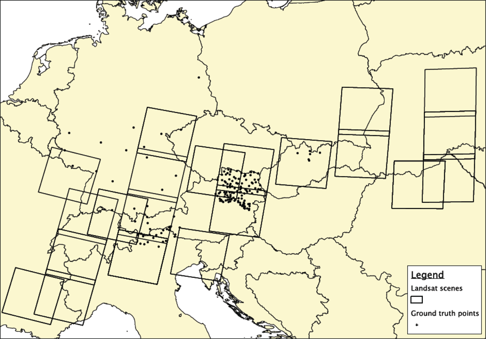
Figure 1 illustrates the location of the analyzed Landsat scenes and the ground truth points. The NASA SCA products were selected over the Landsat acquisitions.
To assess the quality of the EURAC SCA product, the confusion matrix between the EURAC SCA maps and the reference data (Landsat SCA maps, NASA SCA or ground station data) was calculated. The confusion matrix has the form indicated in
Table 1:
Table 1.
Example of confusion matrix used in the validation activities
Table 1.
Example of confusion matrix used in the validation activities
| Date | Reference SCA | |
|---|
|
|---|
| EURAC SCA | Snow | Snow-Free | |
|---|
| snow | a | b | OA (%) |
| Snow-free | c | d |
The commission error for the snow class is calculated as the ratio, b/(a + b), and corresponds to the 1−User Accuracy (UA), where UA = a/(a + b). The omission error for the snow class is calculated as the ratio, c/(a + c), and corresponds to the 1-Producer Accuracy (PA), where PA = a/(a + c).
When one category is dominating (and for most of Europe, this is the case of the “snow-free/snow-free” events in the summer period), the agreement score is not sufficient. To complete the analysis, the Heidke Skill Score (HSS) is then calculated to complete the analysis. The HSS calculates the skill of the compared dataset with regards to a random dataset [
19]. The HSS can be expressed as:
The HSS ranges from −∞ to 1, where the negative values indicate a negative skill, 0 no skill and 1 is the skill of a perfect dataset. When one class is dominating, such as snow-free areas, it is proven that [
18]:
which shows that this score gives more importance to correct classification of snow-covered pixels in the case that “snow-free/snow-free” events are dominating.
In this work, it was decided to compute the scores over the complete data sets, not excluding the so-called summer months (i.e., months when snow presence is reduced). The proposed study area being so large and variable, the duration of the snow-free period is highly dependent on the area location. High mountains obviously contain snow during the entire year, but concerning mid-altitude mountains or continental, snow cover can be also present in different periods. Moreover, as one of the possible applications of the derived SCA maps is related to hydrological purposes, many river basins contain both high mountain areas and low altitude areas, and for this reason, the whole year has been considered.
3.1. Comparison with SCA Maps Derived from Landsat 7 ETM+ Images
A first approach to assess the accuracy of the EURAC SCA algorithm is a comparison with SCA maps derived from Landsat scenes at 30 m resolution. The Landsat SCA maps were derived by using an adapted Landsat snow cover detection algorithm originally developed for MODIS. The algorithm is known to produce highly accurate snow maps even for mountainous areas, which is apart from the spectral characteristics of the sensor, mostly attributable to its high spatial resolution [
21]. It basically follows the standard algorithm using the Normalized Difference Snow Index (NDSI) [
22], including regionally adapted thresholds and an improved cloud mask, with thresholds tuned especially for mountain areas.
For the season, 2005/06, 16 Landsat scenes well distributed over Central Europe (
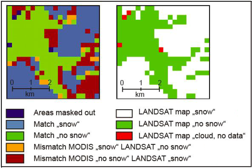
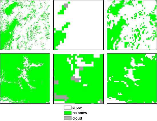
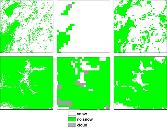
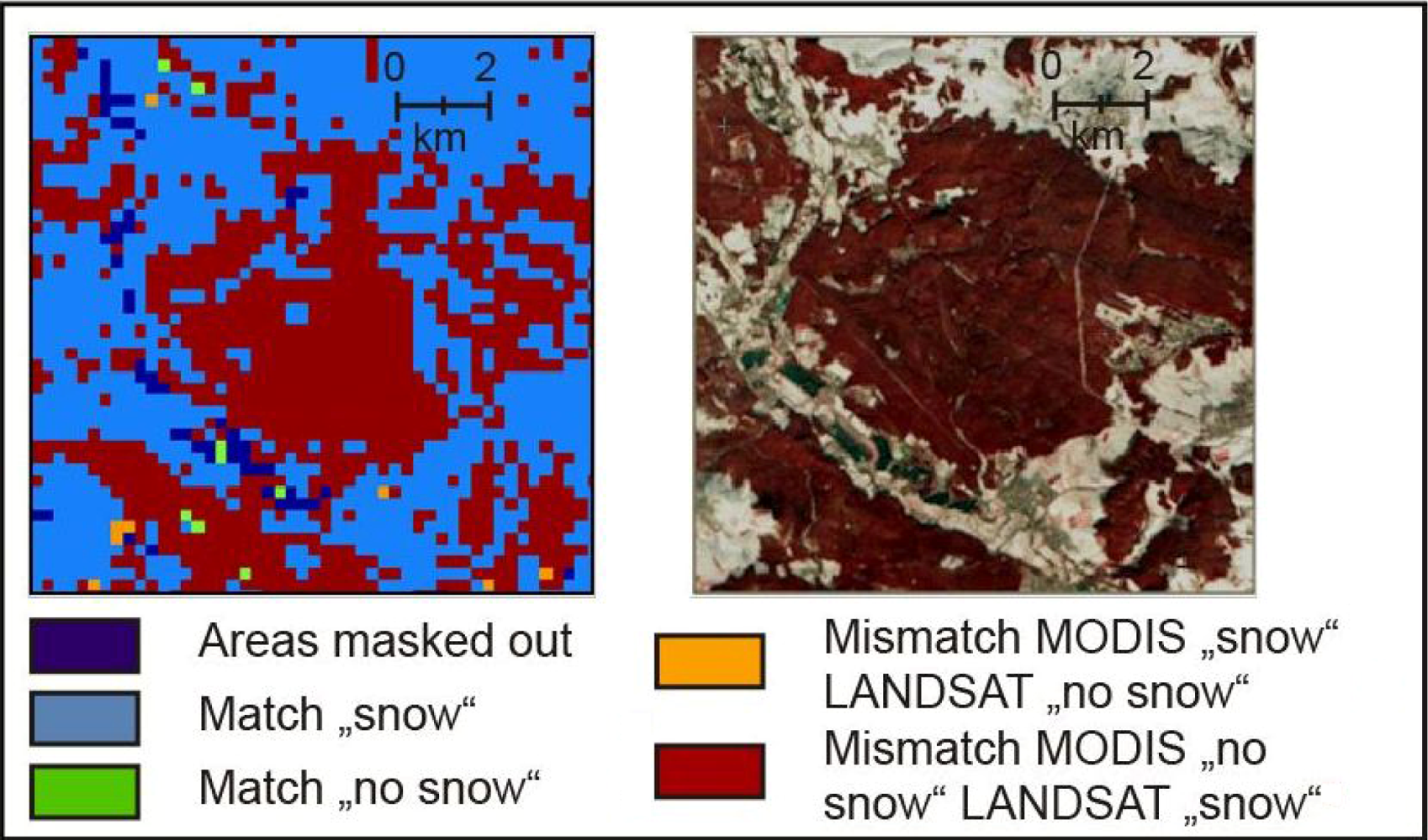
Figure 1) were downloaded, and the SCA maps were generated with the above mentioned algorithm. The choice of the scenes was driven by the intention to cover topographically different landscapes, as well as by the availability of scenes inside the area of interest (AOI) during the investigation period. The selected scenes included images from different areas, such as lowlands, the Carpathians and the Alps, north and south of the Alpine Divide. Since the objective was to estimate the detection accuracy for snow-covered and snow-free area, only the two respective classes were considered, while masking out in both maps the classes without information on the surface conditions, such as “clouds” and “no data”. Concerning the water bodies, there was a difference in the way they are treated in the algorithms; these areas were therefore masked out as well. The Landsat ETM+ sensor has a data acquisition problem since 2003, leading to a striped pattern of unusable data in the images in certain distances east and west of the satellites’ nadir. With the help of masks provided by NASA, these areas were also excluded from the comparison. In a next step, the high resolution Landsat SCA maps were resampled from 30 m to 250 m using the condition that the majority of these almost 70 cells constitute the class of the new resampled cells. These pixels shall contain only the information about the classes of “snow” and “snow-free”. The resampled Landsat SCA map was overlaid with the EURAC SCA map, and an algorithm calculated the share of the matching and non-matching classes, respectively, as indicated in
Figure 2.
The results of sixteen comparisons showed a mean agreement of 88.1% (
Table 2). A closer investigation of the mismatching areas followed to understand origins and locations of problems. The main reasons for mismatching were found to be linked with the following issues (listed from the least probable to the most probable):
Different acquisition times of the two satellites
Problems in detecting snow in shadowed areas
Data inconsistencies on the edge of the Landsat images
Misclassification errors at the cloud borders
Difficulties in detecting snow in forest.
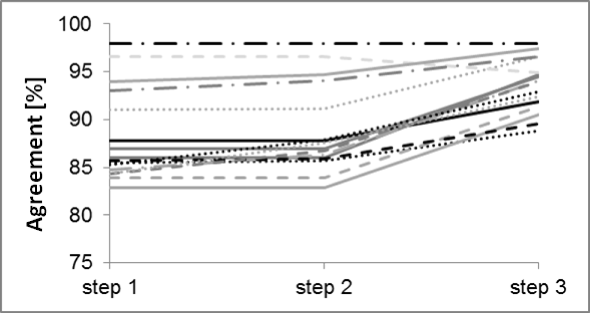
The mentioned problems affect both the MODIS and the Landsat SCA maps, suggesting careful judging of the agreement results. In the comparison, three main steps were considered: step 1, applying masks for clouds, water and Landsat stripes; step 2, additionally applying shadow and cloud edge masks; and step 3, additionally applying a forest mask. Applying these masks, in step 1 around 25% of the pixels are masked, in step 2 the shadow masks can vary between 0.5% and 60% according to the different areas and in step 3 the forest masks can vary between few percentages to 60% according to the different areas. Steps 1 and 3 are reported in
Table 2. The second step constitutes a more objective comparison by masking out shadowed areas, as well as problems at the edge of the Landsat scenes, due to inconsistent swath coverage of the various ETM+ bands. During winter, shadows cover parts of the Landsat scenes, especially in hilly and mountainous terrain, due to the low sun elevation angle at the time of image acquisition. These scarcely or only diffusely illuminated slopes did not allow an easy land cover classification and were one potential source of errors. Since the MODIS sensor experiences different illumination conditions during its acquisition, the shadowed areas could not be compared and were therefore masked out in both maps. Applying these operations on the comparison process the agreement increases by 0.77%. These results indicate a relatively low impact of the shadowed areas, even though there were slight differences according to topographic conditions.
The general agreement areas reveal similar spatial patterns, while there are still residual mismatching areas. These areas are mainly linked to the problem of detecting snow in forest. This motivates the third step in the comparison procedure. To confirm this assumption, additional comparisons considered only the non-forested land. The results show that outside of forested areas, the agreement is, on average, 4.8% higher and reaches an overall agreement of 93.6% (
Table 2). The residual mismatch area of ∼6% may be considered as the result of the interplay of a complex set of factors. These may range from the fact that two remotely sensed sets of data are being compared (different sensors, acquisition times
etc.), to small-scale weather phenomena, like near-ground fog or ground frost, to changing forested areas (differences between the forest maps used in the algorithm and forest stands in reality), the unavoidable presence of mixed pixels, the geocoding accuracy and others. Apart from forest, there is no clear correlation with other types of land cover.
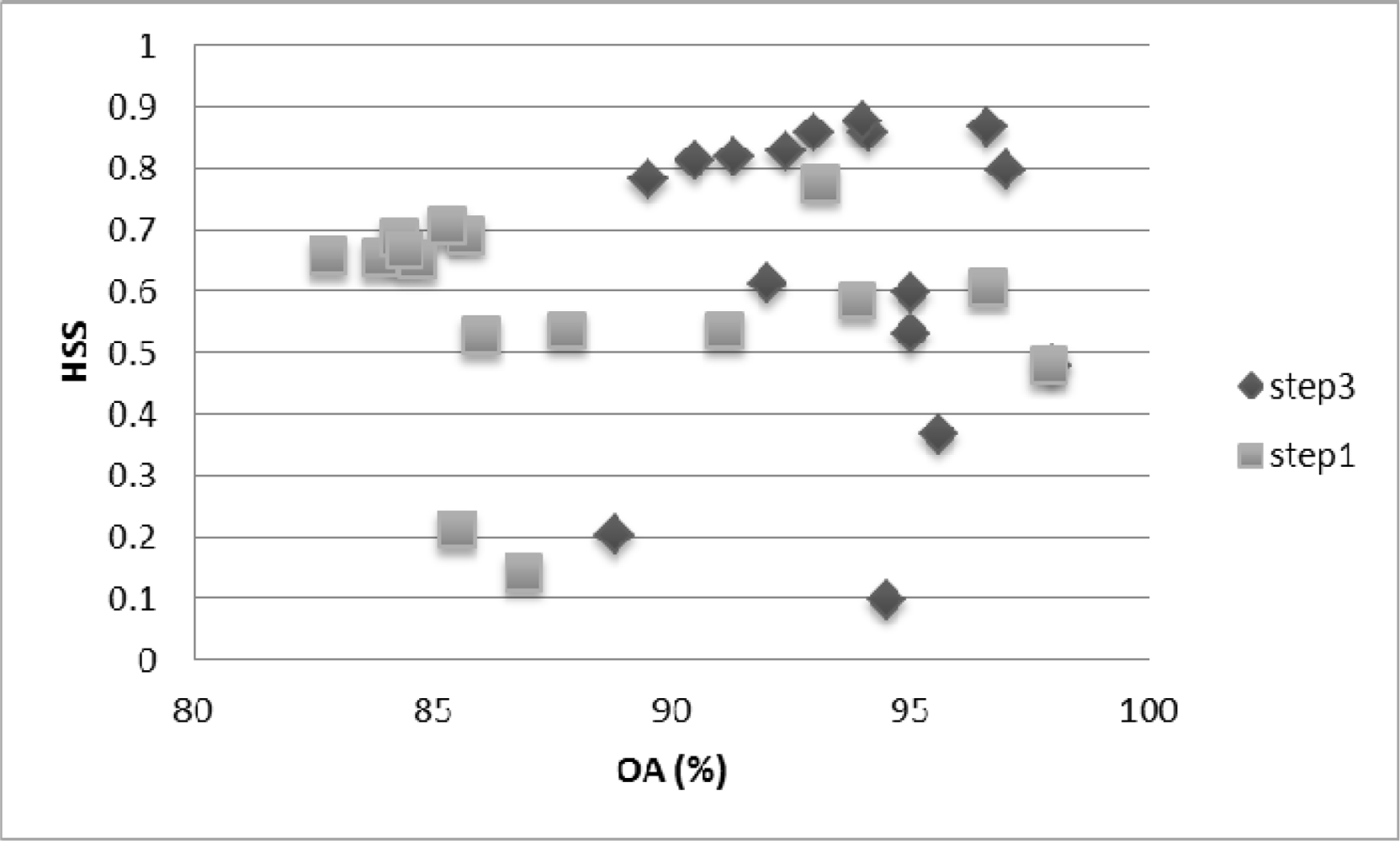
Figure 3 summarizes the three evaluation steps in the comparison between EURAC and Landsat SCA maps.
The HSS score was applied for steps 1 and 3, and the results are illustrated in
Figure 4. The graph indicates that the increasing of the OA from step 1 to step 3 is found also in an increase of the HSS index. The lowest values of HSS are found in both cases for two dates, 20060206_191026 and 20060309_184027.
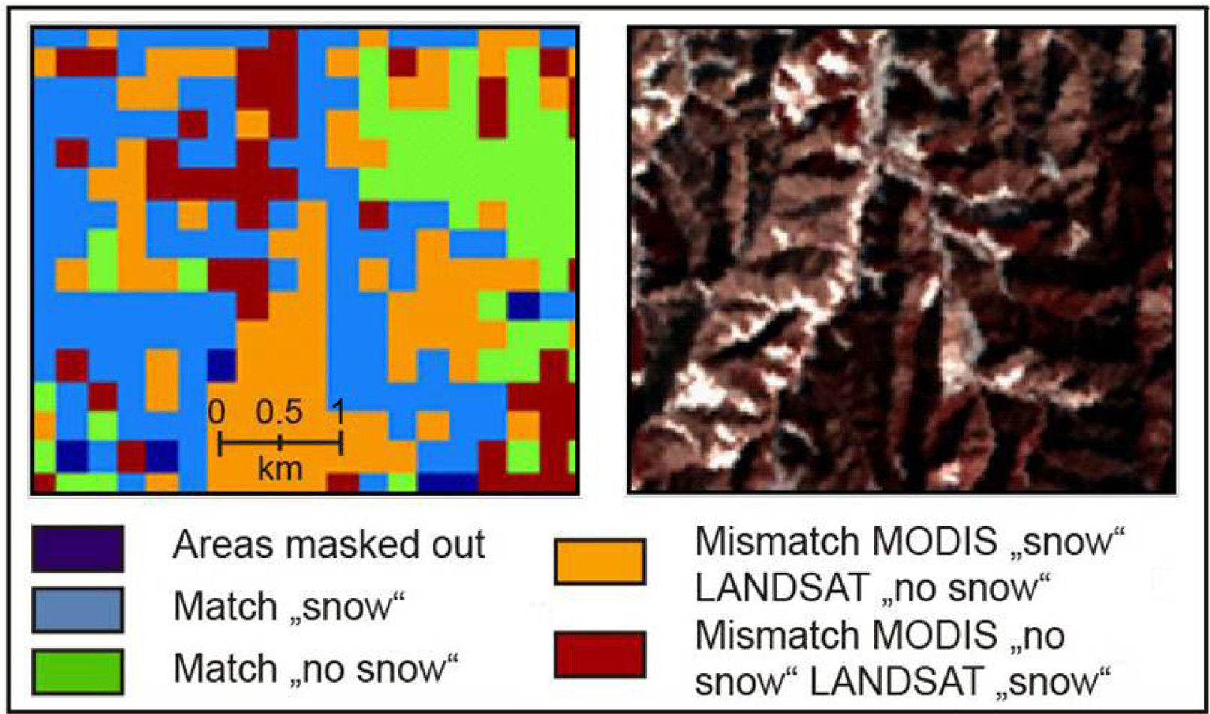
The detection of snow in forest as the major constraint deserves a closer look. Naturally, most problematic are coniferous forest stands. The denser the forest and the less snow remaining on crowns and branches, the harder it gets to detect it. The problem of detecting snow in forest is highlighted in
Figure 5, which is a comparison of the mismatch map of 2 December in 2005 in the Landsat path/row 184/027. The Landsat algorithm correctly classifies all the area as snow covered; on the contrary, the EURAC algorithm classifies data well at the edge of forests and in less dense forest stands, but does not receive enough radiometric contribution of snow in denser forest parts. Difficulties in the validation of MODIS SCA maps in forested sites are also illustrated in other works, as [
23].
One of the main differences between the EURAC and NASA algorithms in the detection of snow under forest is the use of NDSI index (bands for this index are at 500 m). The NASA algorithm adopts a combined use of NDVI and NDSI, which improved the detection of snow in forested areas based on the approach of Klein
et al.[
24]. On the other hand, to preserve the resolution at 250 m, the EURAC algorithm performs the analysis only on NDVI and B1 (blue band). In particular for the B1 band, a multi-temporal approach is proposed comparing B1 in the snow covered images with B1 reference images snow-free, and the changes in reflectances are found to be well correlated to the presence of snow in forest. In any case, they are not the best tool to detect snow in forest, because the NDSI provides a further constrain on NDVI and B1 values, as indicated in [
24]. This results in the discrepancies of the forested areas, which are also found when comparing EURAC SCA maps with NASA SCA maps.
Several scenes show a less strong increase in accuracy after the step 3 operation, suggesting that there are other sources of misclassifications apart from the detection of snow in forest. However, these mismatching areas are not necessarily linked with errors in the EURAC SCA maps, but can also be due to problems of the Landsat algorithm, as shown in
Figure 6, where the Landsat scene is wrongly classified, especially on low illuminated slopes. Similar observations have been made also in well-illuminated areas, where the EURAC results under certain circumstances were found to be correct.
3.2. Comparison EURAC Snow Product—NASA Snow Product
We compared the SCA maps derived from the EURAC algorithm with the NASA SCA maps of MOD10 products. In
Table 3, to indicate the comparison, the date, track and frame from Landsat images are used (e.g., 20060202-195027 indicating an acquisition on 2 February 2006, with the area identified by path 195 and row 27).
The overall accuracy varies between 78% and 98.3%, with an average of 85.4%, where the commission error from the EURAC SCA maps is 4.9% and the omission error 16.2%. When a forest mask is applied, the overall accuracy is increased to 90.2%, where most of the improvement originates from the reduction of the omission error. The use of a forest mask clearly shows that the differences in the two products are due to the treatment of the forested areas and, more precisely, due to the underestimation of snow detection by the EURAC SCA algorithm. As already mentioned in the description of the results, one major difference is that EURAC algorithm to maintain the resolution of 250 m does not include NDSI (500 m), which better constrains, along with NDVI, the detection of snow in forest [
20].
The study of the distribution of omission and commission within forested areas clearly shows that omission is the biggest factor of discrepancy between both EURAC and NASA products, with in average 22.3% of omission error versus 4.9% of commission error. This is also evident when considering the HSS values. For most cases, the HSS ranges between 0.6 and 0.9, while for those images where the discrepancy due to forest is high (e.g., 20060206_191026), the HSS values are found very low between 0.1 and 0.2.
Table 4 summarizes the overall accuracy (OA in %) of the EURAC SCA maps with respect to the Landsat and NASA SCA maps.
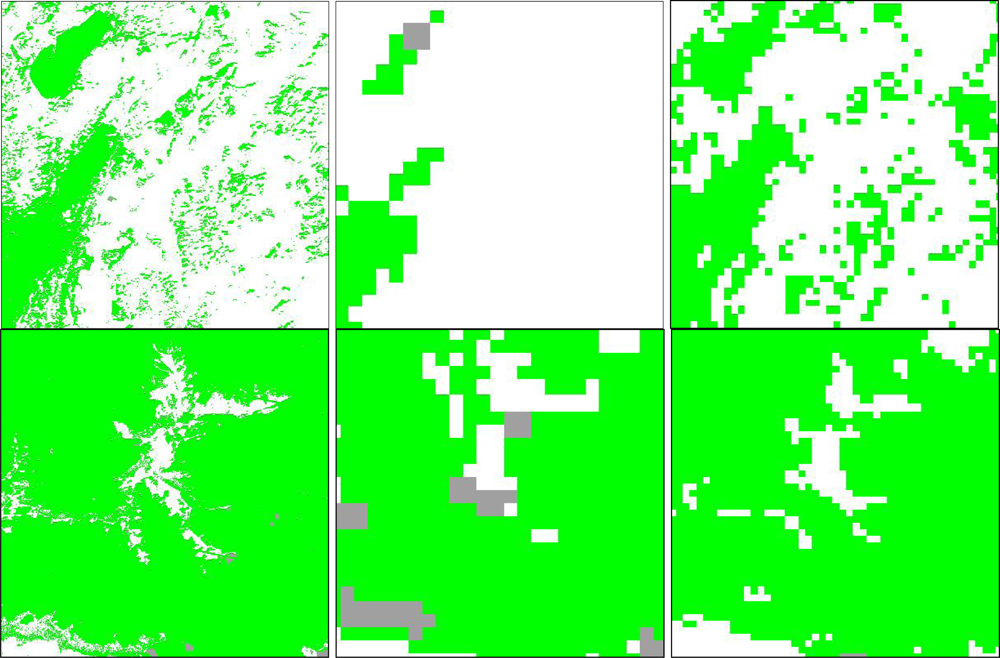
In order to better highlight the advantages derived from the 250 resolution, the Landsat, NASA and EURAC SCA have been compared over areas with the presence of patchy snow. As already indicated in [
25], the 500 resolution of NASA SCA may be ascribed as one of the major sources of snow misclassification. In this preliminary analysis, several windows with size varying from 1,000 to 3,000 Landsat pixels have been localized over patchy snow areas, and the percentages of snow and snow-free areas have been calculated for Landsat, NASA and EURAC SCA maps. Considering then the Landsat SCA as a reference, the root mean square error (RMSE) between Landsat and NASA snow percentages and between Landsat and EURAC snow percentages have been calculated. The RMSE for the NASA SCA is found around 25%, while for EURAC SCA the RMSE decreases up to 16%. From the comparison of RMSE values, as well as from visual inspection (
Figure 7), the EURAC SCA maps seem to better reproduce the snow patterns, mainly due to the improved resolution, thus reducing the likelihood of misclassified pixels.
4. Validation with Snow Depth Data from Meteorological Stations
The EURAC SCA maps were compared to
in situ snow measurements from 148 ground stations in Austria, Germany, Slovakia and Italy in the period from August 2005 to July 2006. The aim of this comparison was:
- (a)
To assess and discuss the overall accuracy of the EURAC SCA maps for the selected regions;
- (b)
To analyze temporal variations of the quality of the EURAC SCA maps;
- (c)
To understand possible error sources.
The available
in situ data from Germany cover Central and Southern Germany (Deutscher Wetterdienst) [
26], the data from Austria are from the Austrian Province of Lower Austria (Lawinenwarndienst Niederösterreich) [
27], the Italian data are from South Tyrol region (Autonomous Provinz Bozen Südtirol/Provincia Autonoma di Bolzano Alto Adige) [
28] and the Slovakian data cover only a part of the entire country (Slovakian Avalanche Centre) [
29]. The whole data set is from 2005 and 2006. It is worthwhile mentioning that continuous data sets are only available for Germany, Lower Austria and Slovakia and for two stations in South Tyrol. Most stations in South Tyrol measure snow only during the winter season. All snow measurements were performed at meteorological
in situ stations, and daily snow depth values are provided with a vertical resolution of ∼1 cm.
The in situ data cover a wide range of different surface types, snow cover conditions and elevation levels, ranging from frequently snow covered mountain areas in South Tyrol to flat regions in Southern Germany and can hence be considered as representative for European conditions.
For each investigated region, the available in situ data are compared to EURAC SCA maps from the Terra satellite acquisition. Snow measurements are usually performed early in the morning, and thus, the late morning acquisition of the Terra satellite better corresponds in time to the in situ snow measurement with respect to the afternoon Aqua acquisition. We have compared snow retrievals from single SCA pixel to the corresponding in situ measurements. Ground data with a snow depth of 2 cm and less are considered as snow-free in the comparison, as light snow coverage can rapidly melt during the day and might thus not reveal the actual snow status at the time of the satellite acquisition.
Overall accuracies for the different regions between the EURAC SCA product and
in situ snow measurements range between 82.4% and 93.7% (
Table 5). For NASA SCA, Parajka and Blösch [
25] reported an accuracy between 88% and 99% under clear sky conditions. It is important to note that in
Table 5, the overall accuracy strongly depends on the relative number of
in situ snow observations compared to snow-free observations included in the analysis. A higher number of
in situ snow observations compared to snow-free observations results in a lower overall accuracy. This is due to lower commission errors compared to omission errors in all selected regions. For these reason, in
Table 5, for both classes (snow and snow-free), the hit rate is reported that is the number of pixels correctly classified over the total number, while the overall accuracy (OA) is an average of the hit rates weighted over the respective number of points.
Mismatches between the EURAC SCA map and
in situ data are lower for snow pixels (from 5% to 10%) as for snow-free pixels (15% to 28%) in all regions. This behavior can be ascribed on one side to the amount of points in snow and snow-free classes, which consequently affects the evaluation of the error classes,
i.e., snow detected as snow-free and snow-free detected as snow. On the other side, the choice of the snow depth to 2 or 5 cm may influence these errors, as well as the OA. In any case, a sensitivity analysis indicates that the changes in the OA when considering 2 cm or 5 cm for snow depth are not found to be significant [
30].
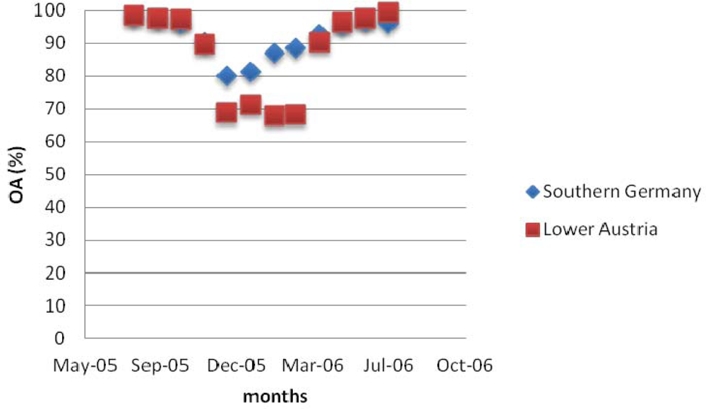
Considering the comparison results for Southern Germany out of 460 stations detecting snow presence, 85.4% were correctly classified as snow and 14.6% were wrongly classified as snow-free by EURAC MODIS. On the other hand, of 2,735 snow-free stations, 95.1% were correctly classified as snow-free and only 4.9% were wrongly classified. For Lower Austria, out of 2,567 stations detecting snow presence, 85.0% were correctly classified as snow and 15.0% were wrongly classified as snow-free. For the 13,607 snow-free stations, 90.3% were correctly classified as snow-free and 9.7% were wrongly classified. These values are on the same order of magnitude as the errors reported for the MODIS NASA standard product in Austria, that is, 3.5% of snow-free stations wrongly classified as snow and 15.8 % of stations detecting snow wrongly classified as snow-free by Parajka and Böschl (2006) [
14]. Stations detecting snow and found as snow-free on the snow maps are about 6% to 10% higher in Slovakia and South Tyrol compared to Germany (
Table 5). This problem will be addressed in the error analysis. We have investigated the temporal variability of the overall agreement of the SCA maps by computing overall accuracies for Southern Germany and Lower Austria on a monthly basis. Both regions measure snow year-round and have a significant amount of monitoring stations. This study was carried out because the accuracy of MODIS-based snow products generally shows a significant seasonal variability [
13,
14]. The accuracies of the NASA standard snow MOD10 and MYD10 products are usually lower at the beginning and end of the snow season [
13,
14]. As an example, the temporal trends for Southern Germany and Lower Austria are reported in
Figure 8. The agreement between the EURAC SCA maps and the snow stations follows a clear seasonal pattern, with the lowest accuracies during the winter months (
Figure 8).
The lowest agreements between the SCA map and
in situ data can be observed in December and January in Southern Germany and from December to March in Lower Austria. In Lower Austria, we can observe a clear decrease of the accuracy in the SCA maps during the beginning and the end of the snow season. This behavior of the SCA maps is in line with temporal accuracy variation reported for the MODIS NASA standard SCA product [
13,
14].
Mismatches between in situ point measurements and spatially averaged satellite data can result from errors of the in situ measurements, due, for example, to a missing quality check on the data, inaccurate satellite products, especially in terms of geocoding accuracy, or from the fact that the physical unit measured at the in situ station is not representative for the entire pixel area. In this study, we investigated whether low overall accuracies for selected stations are due to non-representative in situ stations or if they, rather, indicate detection problems of the proposed SCA algorithm. We therefore computed the overall accuracy for each in situ station in a rather flat region (Germany) and in a mountainous area (South Tyrol). All stations with low overall accuracies were then visually inspected on high-resolution satellite data in order to check if the selected station can be considered as representative for the entire MODIS pixel area (250 m × 250 m).
In South Tyrol, very low accuracies of the SCA maps can be observed for the stations, Ausserrojen, Klausberg, Pens, Rein in Taufers and Stausee Zoggl (
Table 6). All those stations have a common characteristic: they are located along northeastern, northern or northwestern steep mountain flanks and are, therefore, poorly illuminated during the early acquisition time of Terra in the winter season. In the EURAC SCA algorithm, complete shadowed areas are assigned as “unclassified”. This study probably indicates that the shadow masking of the SCA algorithm needs to be more restrictive. In fact, the previously described high omission error (
in situ snow detected as snow-free; see results related to the overall accuracy) of the SCA map in South Tyrol is likely due to snow underestimations in shadowed areas. In Southern Germany, only two stations (Frankfurt Airport and Zugspitze) have lower accuracies compared to other stations in the same region (
Table 6). The station, Frankfurt, is situated close to a major landing strip of the Frankfurt Airport, which is regularly snow-ploughed in winter. The
in situ snow measurements might thus not always be representative for the entire pixel area. The same is valid for the
in situ station, Zugspitze. Here, snow measurements are performed on top of the highest peak of Germany, which is surrounded by steep mountain flanks. The snow measurements on top of the mountain, hence, do not reflect the snow situation of a larger area (250 m × 250 m).
Considering the results of the ground truth validation study, the following considerations emerge: The 250 m EURAC SCA map appears to be very accurate in Lower Austria and Southern Germany, with an overall accuracy of 90% and 94% compared to in situ snow measurements. Similar high accuracies are only reported for the NASA standard 500 m snow product in Austria.
The error class (in situ snow detected as snow-free) ranges from 6% to 10%, with higher values in South Tyrol and Slovakia than in Southern Germany and Austria. We have observed low overall accuracies for those ground stations in South Tyrol, which are located in mountain shadows during the early Terra acquisition in winter. This behavior points to problems detecting snow in shadow areas in the EURAC SCA algorithm and could explain the observed omission errors. Single measurement stations outside potential shadowing errors in South Tyrol have overall accuracies between 75% and 99%, which is nevertheless a promising result for the performance of the SCA algorithm in very rough terrain.
5. Conclusions
A new algorithm for derivation of snow maps from MODIS images at 250 m resolution was validated by using 16 high resolution Landsat 7 ETM+ images and ground measurements from 148 snow stations.
The results of the comparison with Landsat/ETM+ images indicate a mean overall accuracy of around 88.1%. The accuracy depends strongly on forest coverage, while in open areas, the accuracy is the highest with 93.6%.
The detection of snow in forest is more reliable when also the NDSI is used as indicated in Klein
et al.[
24]. This index has not been considered in this analysis, because it is based on 500 m resolution MODIS bands. The same behavior was found in the comparison with NASA MODIS SCA, where the accuracy is 90.2% and drops to 85.4% in forested areas.
In the comparison with ground measurements, the EURAC snow cover maps (SCA) maps have reached an accuracy of around 93.7%. In some cases, in very rugged terrain with northern exposition, the accuracy decreases to around 82.4%, mainly due to the low values of reflectances, which make the snow detection very difficult based only on the 250 m bands.
Further validation activities will include the analysis of longer time series of EURAC SCA maps with ground measurements, as well as closer investigation of other important factors, such as geolocation accuracy.
To use a 250 m resolution map is important for two main reasons, because it is really based on the data at 250 m and not on methodologies and calibration with other data as, for example, the ones used to derive the fractional snow covers. This means that the algorithm is quite fast, being based on hard thresholds (decision trees), and can be easily adapted to different regions. The problem of forest is a known problem. Improvement, as demonstrated [
30], can be obtained by using the NDSI, which is contained in the quality layer. In summary, this means that you have a very flexible algorithm, where you can have a “real” 250 m map, and additionally, for the areas where there could be a problem, you can used the quality flag, which is based on NDSI.
Actually, the data have been delivered to the Joint Research Centre in the framework of a pilot project “Provision of Daily Snow-Cover Map Products in Near Real-Time as Input for the European Flood Alert System (EFAS)” for improving flooding forecasting in Central European catchments [
30]. The SCA maps are also provided on a daily basis and in near real-time, based to the Autonomous Province of Bolzano-Civil Protection office, mainly used in alerting systems for avalanches and for touristic information.
MODIS sensors are already working, since five years after the expected lifecycle. Even though a fixed end-of-life is not yet defined, as a successor of MODIS, the EURAC receiving station is already receiving and processing datasets from a Visible/Infrared Imager Radiometer Suite (VIIRS) sensor on board the NASA Suomi National Polar-orbiting Partnership (NPP) satellite. This sensor will substitute MODIS in the next 20–30 years [
31]. Among VIIRS products, SCA maps are also foreseen at 400 m resolution. In the period of contemporary acquisitions of MODIS and VIIRS, the EURAC SCA maps can be used as a support to validate and to downscale the NPP SCA maps.

 ,
, 
