The Temporal-Spatial Distribution of Shule River Alluvial Fan Units in China Based on SAR Data and OSL Dating

Abstract

Alluvial fans in arid and semi-arid regions can provide important evidence of geomorphic and climatic changes, which reveal the evolution of the regional tectonic activity and environment. Synthetic aperture radar (SAR) remote sensing technology, which is sensitive to geomorphic features, plays an important role in quickly mapping alluvial fan units of different ages. In this paper, RADARSAT-2 (Canada’s C-band new-generation radar satellite) and ALOS-PALSAR (Japan’s advanced land observing satellite, phased array type L-band SAR sensor) data, acquired over the Shule River Alluvial Fan (SRAF), are used to extract backscattering coefficients, scattering mechanism-related information, and polarimetric characteristic parameters. The correlation between these SAR characteristic parameters and fan units of the SRAF of different ages was studied, and the spatial distribution of fan units, since the Late Pleistocene, was extracted based on the Maximum Likelihood classification method. The results prove that (1) some C-band SAR parameters can describe the geomorphic characteristics of alluvial fan units of different ages in the SRAF; (2) SAR data can be used to map the SRAF’s surface between the Late Pleistocene and the Holocene and to extract the spatial distribution of fan units; and (3) the time-spatial distribution of the SRAF can provide valuable information for tectonic and paleoenvironmental research of the study area.

1. Introduction

Alluvial fans in arid and semi-arid areas are important recorders of both tectonic and climatic signals [1–8]. Fan units of varying ages, with different geomorphic features, can contain vast amounts of information for the study of paleoclimatic and paleoenvironmental changes [2,8–10]. Some of the most important pieces of such information are the temporal-spatial distribution characteristics of alluvial fan geological units.

Remote sensing has become a significant tool for the study of alluvial fans [11–14]. Due to its capability to record multi-polarization, multi-band, and high-resolution microwave backscattering returns, and due to its sensitivity to most geomorphic features (gravel size, surface roughness, surface desert pavement development, and bar-and-swale structure) of alluvial fans in arid and semi-arid areas, synthetic aperture radar (SAR) has played an important role in mapping the surface of alluvial fans [15–22].

In earlier studies, Farr et al. analyzed the backscattering coefficient characteristics of the alluvial fans located on Kunlun Mountain, China, based on Spaceborne Imaging Radar-C (SIR-C) SAR data and concluded that alluvial fan units of relatively different ages can be effectively segmented by utilizing SAR backscattering coefficients [15]. Since that study, many studies of alluvial fans have been conducted using SAR data. An increasing amount of SAR parameters that are sensitive to the geomorphic features of alluvial fans’ surfaces, such as surface roughness and gravel size, have been analyzed, and many models and inversion methods have been proposed to extract these features. Furthermore, the characteristics of these geomorphic features within different fan units in the study areas have also been discussed [16–20,23–25].

Recently, SAR has entered into a “golden age” of study. More than 15 space-borne SAR sensors are in operation today [26]. An increasing amount of SAR data with diverse modes can be collected from space-borne SAR sensors, including TERRASAR-X (Germany’s X-band high-resolution radar satellite) [27], RADARSAT-2 [28], and ALOS-PALSAR [29]. Furthermore, as SAR theories and techniques have rapidly developed [30], many information extraction methods have been proposed. Detailed information concerning the ground surface’s sensitivity to geomorphic features can be obtained, particularly information concerning the scattering mechanism [31–33]. Consequently, it is necessary to conduct further analyses of the expression of SAR parameters on alluvial fan units of varying ages and to exploit the application potential of SAR on the study of alluvial fans, particularly on the study of paleoenvironmental change, based on alluvial fans.

In this paper, the relationship between these SAR parameters and the Shule River Alluvial Fan (SRAF) units of different ages was studied. Moreover, the temporal-spatial distribution of fan units was extracted and analyzed. Based on this geological information, we try to better understand the following questions: (1) Which parameters extracted from SAR data are associated with the geomorphic features of alluvial fan units and can be used to map them? (2) What is the characteristic of the SRAF units’ temporal-spatial distribution, and what is the correlation of that distribution to tectonic activities and paleoenvironmental changes?

2. Study Area (SRAF) and Data

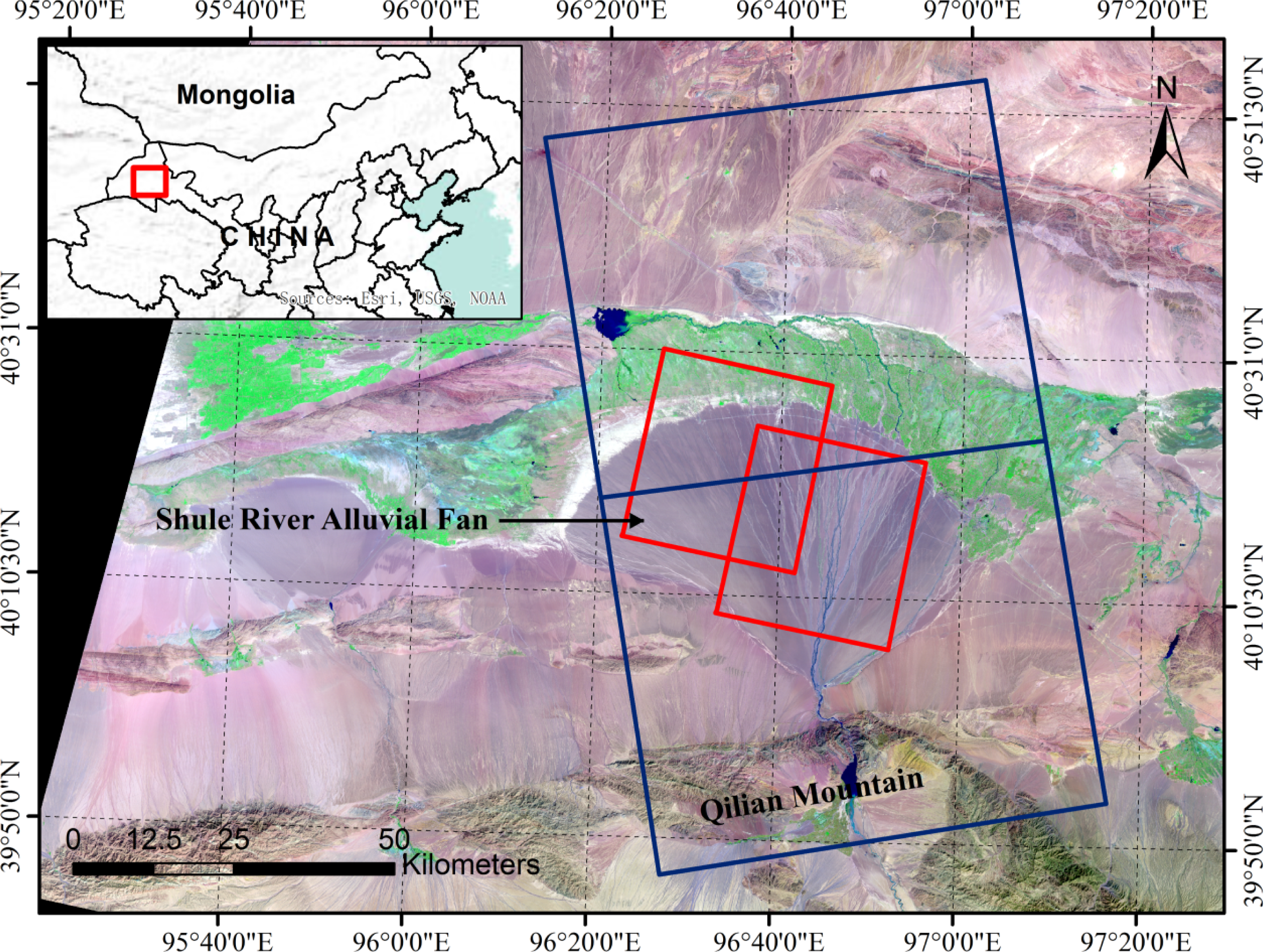
2.1. Location and Geologic Setting of the SRAF

Located in Northwest China, the SRAF, with an area of approximately 2,400 km², was chosen as the study area in this study. This large alluvial fan lies in the range front of the north Qilian Mountains and in the east end of the Alty Tagh Fault zone. Figure 1 shows the location of the SRAF (E: 96°10′–97°10′/N: 40°00′–40°30′). The SRAF developed in a left-lateral strike-slip domain setting provided by the Sanwei Mountain Fault and the Dongbatu Mountain Fault, which are associated with the general Altun Tagh Fault structure and the uplift of the Qilian Mountains [34,35]. This area is primarily composed of the Middle-Late Pleistocene Jiuquan Gravel and Gobi Gravel formations. Late Pleistocene and Holocene sedimentary rocks are exposed widely.

The surface of the SRAF is flat and integrated, tilting gradually from south to north, with a slope of 11.5°. Originating from west of the Qilian Mountain, the Shule River flows northward through the study area. The study area is very arid, with an average annual precipitation of 39.6–63.4 mm/a and an average annual evaporation of 2,469–2,869 mm/a [36]. Overall, the scale and position make this particular alluvial fan an ideal study area for remote sensing alluvial fan research.

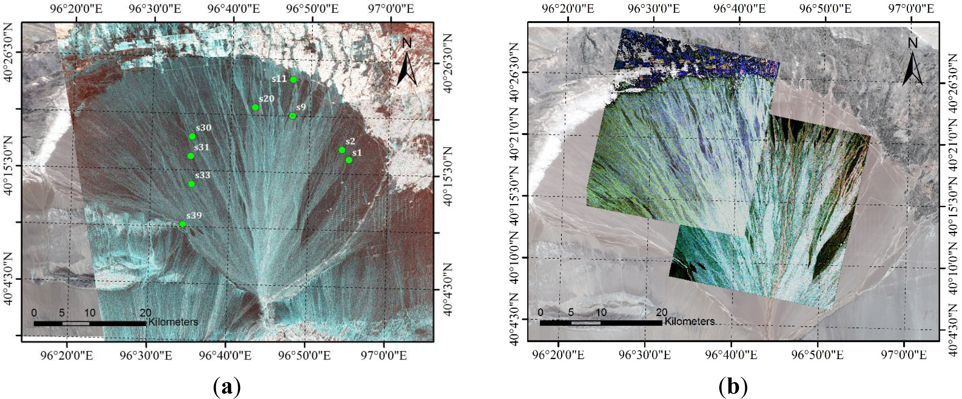
2.2. SAR Dataset of the SRAF

The SAR dataset used in the SRAF study area was composed of two L-band dual-polarization ALOS-PALSAR images acquired on 10 October 2009, and two C-band full-polarization RADARSAT-2 images acquired on 8 June 2010, and 18 November 2011. The footprints of the RADARSAT-2 and ALOS-PALSAR SAR dataset are shown as red and blue rectangles, respectively in Figure 1. The incidence angles of the ALOS-PALSAR and RADARSAT-2 images are 39° and 37°, respectively, and the resolutions are 15 m and 8 m, respectively.

Table 1. The parameters of the synthetic aperture radar (SAR) dataset of the Shule River Alluvial Fan (SRAF).

SAR Sensor	Time	Band	Polarization	Resolution (m)	Incidence Angle (degree)
ALOS-PALSAR	10 October 2009	L	HH/HV	15	39
ALOS-PALSAR	10 October 2009	L	HH/HV	15	39
RADARSAT-2	8 July 2010	C	HH/HV/VH/VV	8	38
RADARSAT-2	18 November 2011	C	HH/HV/VH/VV	8	37

lists the detailed parameters of the collected SAR data. Although the acquisition dates are different, the influences on the arid geomorphic features caused by a temporal difference of two years can be ignored when considering the very long time period during which geomorphic change occurs.

Figure 2a,b is the red-green-blue (RGB) pseudo-color composite images of the ALOS-PALSAR and RADARSAT-2 data in the SRAF, respectively. The red, green, and blue colors in Figure 2a represent the backscattering coefficient combinations of the HV, HH − HV, and HH channels of the ALOS-PALSAR data, respectively, and the red, green, and blue colors in Figure 2b represent the backscattering coefficient combinations of the HH-VV, 2HV, and HH + VV channels of the RADARSAT-2 data, respectively, based on Pauli decomposition.

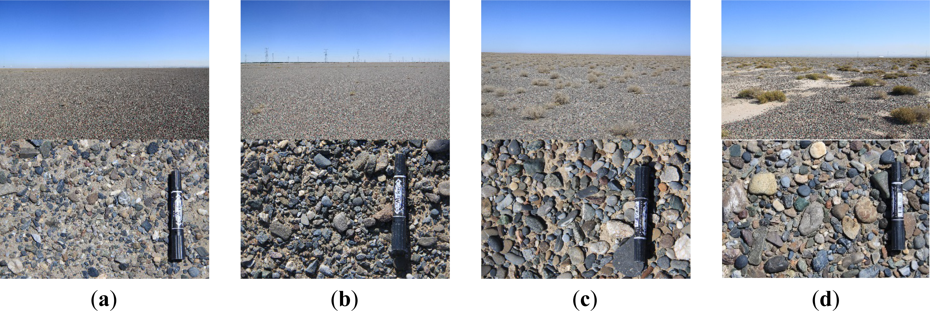
2.3. Geological Survey Data of the SRAF

Two field investigations of the SRAF were conducted in July 2011 and May 2012. The geomorphic parameters, chemical element, and mineral compositions of approximately 130 samples are analyzed. In addition, the age of some of these samples, determined using the optically simulated luminescence (OSL) dating method [37], was also obtained.

OSL method, proposed by Huntley, is a method used to determine the length of time since the sediment was last exposed to sunlight. The principle of OSL dating is that the length of time sediments have been buried can be determined from the quantity of light emitted. In other words, the older a deposit is, the more photons it will release when exposed to light in a laboratory. The equation is as follows:

$$A_{\mathit{age}}=D_E/D$$

(1)

Where A_age is the age of sample, D_E is the radiation dose needed by the natural accumulation of stimulated luminescence, D the radiation dose of α, β, and γ released by ²³⁸U, ²³²Th along with their degenerations in unit time, the radiation dose of β and γ released by ⁴⁰K and little radiation dose released by a small amount of cosmic rays. As the alluvium exposed to the surface of the SRAF is the object of this study, the samples for OSL dating were collected at approximately 10–15 cm below the surface. The positions with obvious difference in the remote sensing images are often selected as the locations of the samples for OSL dating, combined the geological data and field observation results. They are designated as green points in Figure 2a. This dating information indicates the time of the last alluvial event at the sample location and can, therefore, be used to estimate the formation period of the corresponding alluvial fan units.

Based on the results of the OSL dating, the sediments exposed on the SRAF’s surface primarily formed during the later portion of the Late Pleistocene (Q3) and during the Holocene (Q4). By combining the dating information and the covering and cutting features of the alluvial fan surface based on the SAR data, it can be concluded that the SRAF’s surface can be mapped into four fan units. The oldest of these units formed during the Late Pleistocene and is denoted as Unit-1, whereas the other three alluvial fan units formed during the Holocene and are denoted as Unit-2 to Unit-4. The geomorphic characteristics of the fan units’ surfaces are each unique and are listed below. Photographs of these fan units are shown in Figure 3, and brief descriptions of their surface appearances and geological ages are listed in

Table 2. The geomorphic features of fan units of the SRAF.

Fan Unit	Age	Surface Appearance	Desert Pavement Development	Gravel Characteristics	Relative Coverage *
Unit-1	∼11.3 ka Late Pleistocene	Smooth surface; nonexistent bar-and-swale morphology	Well developed	Very small size and poorly rounded gravel	100%
Unit-2	∼5.6 ka Middle Holocene	Smooth surface; nonexistent bar-and-swale morphology	Well developed	Small size and poorly rounded gravel	90%
Unit-3	0.8∼1.2 ka Late Holocene	Nearly smooth surface, with remnants of bar-and-swale pattern	Well developed	Medium size and medium-rounded gravel	50%
Unit-4	0.3∼0.6 ka Nearly present	Remnants of the abandoned gulch structure, with channels with finer-grained sand	Medium	Large size and well-rounded gravel	25%

^*Retative coverage is defined as a percentage of the covering area of a geological unit estimated form the spatial distribution to the entire study area. The estimated areas of each unit include both the region exposed to the surface and the region covered by the younger fan units.

.

Unit-1

Unit-1 (Figure 3a) formed approximately 11.3 ka ago according to the OSL dating results, indicating that it formed at the end of the Late Pleistocene. The sample measured in Unit-1 is S11 (11.29 ± 0.17 ka) in Figure 2a. In this sample, gravel with poor roundness is tightly packed and forms a mature desert pavement (high gravel coverage). The gravel in this unit is the smallest gravel in size among the four units. The surface is smooth and characterized by nonexistent bar-and-swale morphology.

Unit-2

Unit-2 (Figure 3b) formed at approximately 5.6 ka, during the Middle Holocene, and the sample analyzed from this unit is S1 (5.60 ± 0.13 ka). The geomorphic features in this sample are similar to those of Unit-1, with geomorphic features of poor rounded gravel, mature desert pavement and nonexistent bar-and-swale. The gravel size at the surface is larger than that in Unit-1.

Unit-3

Unit-3 (Figure 3c) formed approximately 1.0 ka ago. The OSL dated samples in this unit are S9, S30, S31, S33, and S39 (from 0.82 ± 0.03 ka to 1.20 ± 0.08 ka). As opposed to Unit-1 and Unit-2, Unit-3 and the subsequent Unit-4 are represented by many gullies with a radiating shape. The surface is slightly uneven, with remnants of a bar-and swale pattern, and the degree of gravel coverage is high. The gravel exposed at the surface is of medium roundness and is larger than that of Unit-1 and Unit-2. In addition, the surfaces of Unit-3 and the subsequent Unit-4 are sparely covered with dry and low shrubs, most of them are Alhagi sparsifolia (camelthorns), one of the typical drought-avoiding plants.

Unit-4

Unit-4 (Figure 3d) is the youngest unit analyzed in this study and is also represented by many radiating gullies. The OSL dating results of the samples in this unit (S2, S20) indicate that it formed approximately 0.5 ka ago (from 0.31 ± 0.04 ka to 0.59 ± 0.02 ka). The alluvium in this deposit is generally distributed as remnants of a gulch structure, with bars of well-rounded and large gravel and with swales (channels) consisting of finer-grained sand. The degree of desert pavement development is medium.

3. SAR Parameter Characteristics of the SRAF Units

Geomorphic features, such as gravel size, desert pavement development (gravel coverage), and bar and swale structure, vary among the different fan units of the SRAF. Generally, the gravel size reflect the stream gradient and flow velocities. The larger the gravel size indicate the higher stream gradient and higher flow velocities.

Many parameters derived from SAR data can be used to describe these features of alluvial fan surfaces because of the sensitivity of SAR data to geomorphic features, including the backscattering coefficient, the degree of polarization, the polarimetric correlation coefficient, and the scattering mechanism-related parameters. In this section, we will discuss how these parameters describe the surfaces of alluvial fans in arid and semi-arid areas, and we will analyze the relationship of these parameters with the SRAF units of varying ages.

3.1. SAR Data Preprocessing and Parameter Extraction Methods

3.1.1. SAR Data Preprocessing

Before obtaining the parameters sensitive to geomorphic features from the SAR data, SAR data preprocessing, such as absolute radiometric calibration, filtering, geocoding, and mosaic was necessary. The absolute radiometry-calibrated backscattering returns can be derived by using the sigma lookup table (LUT) files. For suppressing the speckle noise of SAR images, a box car filter with a window of 7 × 7 was applied to the RADARSAT-2 and ALOS-PALSAR data in this study. In addition, these SAR data were coarsely geocoded using the geocoding information provided by the data products, therefore were finely geocoded based on a fine-geocoding base map. Finally, based on the geocoding SAR images, a mosaic operation was applied for the generation of large-area and seamless SAR images of the SRAF.

3.1.2. Backscattering Coefficients of Typical Polarization States

The backscattering coefficients of different polarization states contain rich information concerning the observed targets. Several parameters of linear polarization states (HH, HV, VH, and VV) can be obtained directly from the SAR data. For polarimetric SAR data, backscattering coefficients with any type of polarization state can be obtained by utilizing the polarization basis transformation [38]. The polarization basis transformation is shown in Equation (2):

$$[S_{(p,q)}]={[U_{(p,q)\to (h,v)}]}^T\hspace{0.17em}[S_{(h,v)}]\hspace{0.17em}[U_{(p,q)\to (h,v)}]$$

(2)

where [S_(h,v)] is the scattering matrix with a horizontal-vertical (h,v) linear polarization orthogonal basis, [S_(p,q)] is the scattering matrix expressed by the (p,q) polarization orthogonal basis, and [U_{(h,v)→(h,v)}] is the basis transformation matrix shown in Equation (3):

$$[U_{(p,q)\to (h,v)}]=\left[\begin{array}{cc}\text{cos}\hspace{0.17em}\varphi & -\text{sin}\hspace{0.17em}\varphi \\ \text{sin}\hspace{0.17em}\varphi & \text{cos}\hspace{0.17em}\varphi \end{array}\right]\hspace{0.17em}\left[\begin{array}{cc}\text{cos}\hspace{0.17em}\tau & i\hspace{0.17em}\text{sin}\hspace{0.17em}\tau \\ i\hspace{0.17em}\text{sin}\hspace{0.17em}\tau & \text{cos}\hspace{0.17em}\tau \end{array}\right]$$

(3)

where $\varphi \in [-\frac{\pi }{2},\hspace{0.17em}\frac{\pi }{2}]$ is the orientation angle and $\tau \in [-\frac{\pi }{4},\hspace{0.17em}\frac{\pi }{4}]$ is the ellipticity. The typical polarization states are linear polarization states and circular polarizations, described by τ = 0 and $\tau =\pm \frac{\pi }{4}$ respectively.

3.1.3. Scattering Mechanism-Related Parameters

The advantage of polarimetric SAR data is its capability to obtain scattering mechanism-related information concerning observed targets by using polarimetric target decomposition methods. The H/A/α model [31,32,38] is commonly used and was adopted in this study to extract scattering mechanism-related parameters and a brief description of this model is given as follows.

The H/A/α model is based on the Hermitian coherency matrix T₃, which is formed by k·k^*T, where k is the target scattering vector $k={[S_{\mathit{hh}}\hspace{0.17em}\sqrt{2}{S}_{\mathit{hv}}\hspace{0.17em}{S}_{\mathit{vv}}]}^T$, the operation *T means conjugate transpose. The coherency T₃ matrix can be written as follows based on the eigenvalue decomposition:

$$T_3=\sum _{i=1}^3{\lambda }_i\hspace{0.17em}{u}_i\cdot u_i^{*T}$$

(4)

where the real numbers λ_i are the eigenvalues, u_i are the unit target vector and can be written as the following form:

$$u_i={[\begin{array}{ccc}\text{cos}\hspace{0.17em}{\alpha }_i{e}^{j{\varphi }_1}& \text{sin}\hspace{0.17em}{\alpha }_i\hspace{0.17em}\text{cos}\hspace{0.17em}{\beta }_i{e}^{j{\varphi }_2}& \text{sin}\hspace{0.17em}{\alpha }_i\hspace{0.17em}\text{cos}\hspace{0.17em}{\beta }_i{e}^{j{\varphi }_3}\end{array}]}^T$$

(5)

Some key parameters, such as the scattering-type angle (α), coherency entropy (H), anisotropy (A), target orientation angle (β) and target phase angle (Φ_i,i = 1,2,3) can been introduced based on the parameters of eigenvalues and eigenvectors. Entropy (H) and anisotropy (A) are obtained from eigenvalues λ_i and given by:

$$H=-\sum _{k=1}^3{P}_k\hspace{0.17em}{\text{log}}_3\hspace{0.17em}{P}_i\hspace{0.17em}\hspace{0.17em}\hspace{0.17em}\hspace{0.17em}\hspace{0.17em}\hspace{0.17em}\hspace{0.17em}{P}_i=\frac{{\lambda }_i}{\sum _{i=1}^3{\lambda }_i}\hspace{0.17em}\hspace{0.17em}\hspace{0.17em}\hspace{0.17em}\hspace{0.17em}\hspace{0.17em}\hspace{0.17em}\hspace{0.17em}\hspace{0.17em}\hspace{0.17em}\hspace{0.17em}\hspace{0.17em}\hspace{0.17em}A=\frac{{\lambda }_2-{\lambda }_3}{{\lambda }_2+{\lambda }_3}$$

(6)

Entropy (H) is a global measure of the distribution of the components of the scattering process and can be used to indicate the complexity and randomness of the scattering types. A high value of anisotropy (A) in the intact region indicates that only one dominant scattering type occurs in that region. The variables (α) and (β) indicate the scattering type angle and orientation angle of the observed targets, respectively. They are given by:

$$\alpha =\sum _{k=1}^3{P}_k\hspace{0.17em}{\alpha }_k;\hspace{0.17em}\hspace{0.17em}\hspace{0.17em}\hspace{0.17em}\hspace{0.17em}\hspace{0.17em}\hspace{0.17em}\hspace{0.17em}\hspace{0.17em}\hspace{0.17em}\hspace{0.17em}\hspace{0.17em}\hspace{0.17em}\hspace{0.17em}\beta =\sum _{k=1}^3{P}_k\hspace{0.17em}{\beta }_k$$

(7)

3.1.4. Polarimetric Parameters of the SAR Data

In addition to the backscattering coefficients and scattering mechanism-related information, some polarimetric parameters can also be extracted from the full-polarization SAR data, including the degree of polarization and the polarimetric correlation coefficient [38].

After an electromagnetic wave is scattered by the observed objects, a depolarization effect is often produced. This effect is expressed as the ratio of the polarized power to the total power. The degree of polarization ranges from 0 to 1, where 1 designates a completely polarized wave, 0 designates an un-polarized wave, and values between 0 and 1 designate partially polarized waves. In terms of the Stokes parameters, the degree of polarization is given by:

$$p=\frac{\sqrt{\sum _{i=1}^3{g}_i^2}}{g_0}$$

(8)

where g₀, g₁, g₂, and g₃ represent the four components of the Stokes vector of electromagnetic echoes.

The polarimetric correlation coefficients describe the relationship between two polarization states and are also important pieces of information that reflect the features of observed targets. Generally, co-polarization correlation coefficients are used and defined as follows:

$${\rho }_{\mathit{ppqq}}=\frac{\langle S_{\mathit{pp}}{S}_{\mathit{qq}}^{*}\rangle }{\sqrt{\langle {\left|S_{\mathit{pp}}\right|}^2\rangle \langle {\left|S_{\mathit{qq}}\right|}^2\rangle }}$$

(9)

where p and q are two orthogonal polarization states. The linear polarimetric correlation coefficient between HH and VV polarization states and the circular polarimetric correlation coefficient between RR and LL polarization states are analyzed in this study, where R and L designate right-hand and left-hand polarizations, respectively.

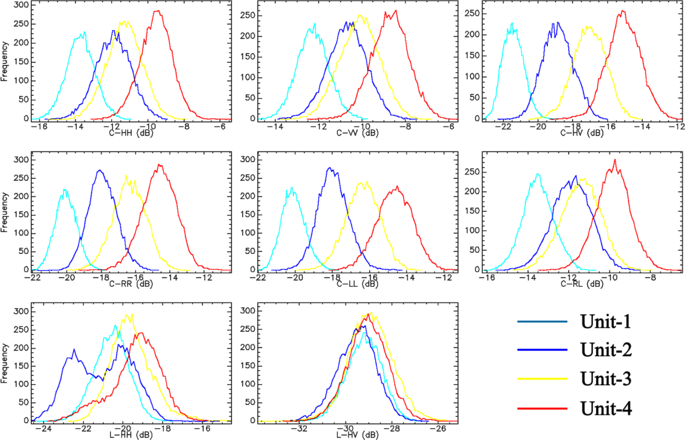
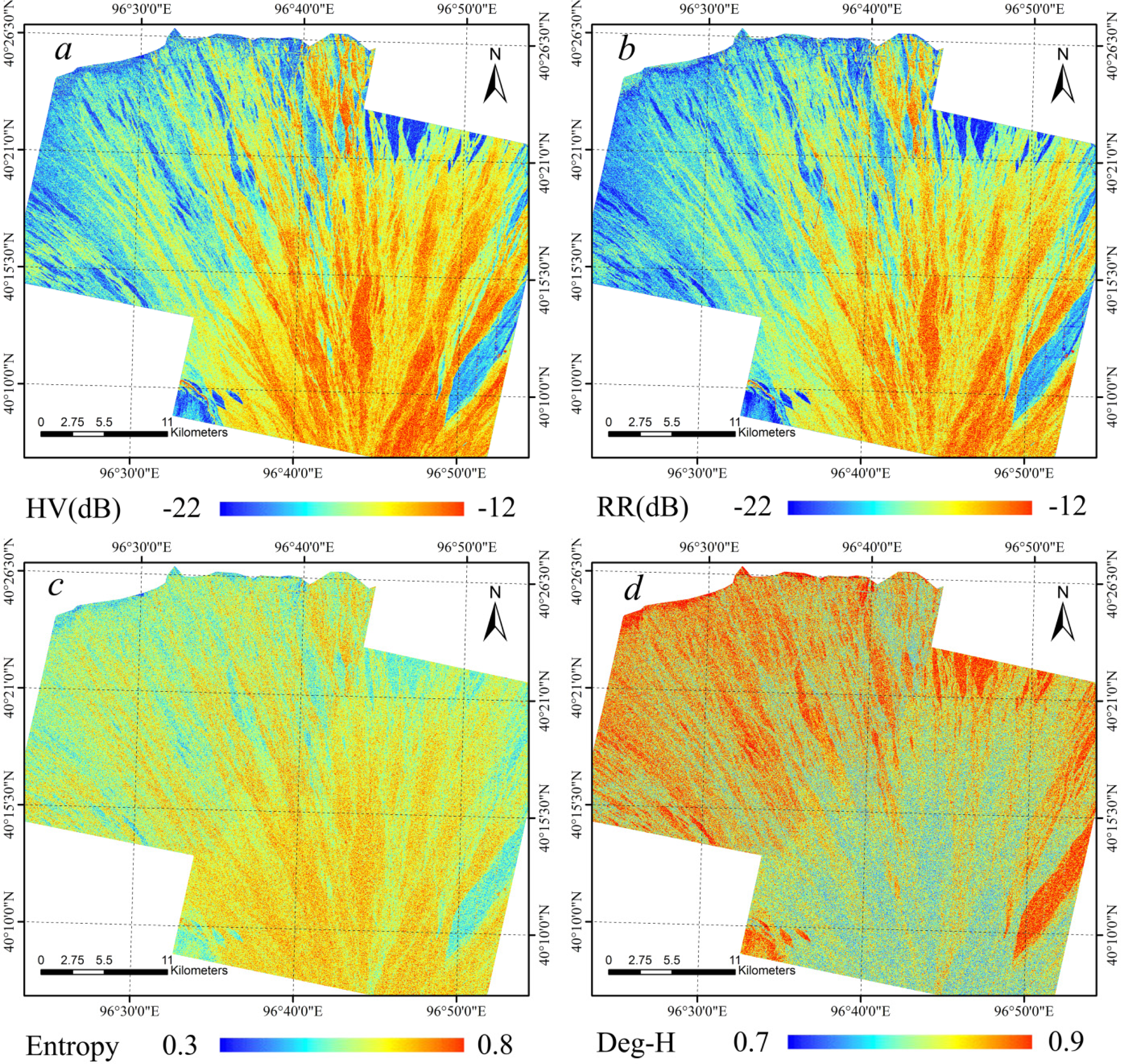
3.2. Backscattering Coefficients of the SRAF Units

Backscattering coefficients for bare ground are sensitive to two factors: surface structure and moisture. Because the SRAF is located in an arid area, the surface is quite dry, the backscattering coefficients in this area are therefore most likely sensitive to surface roughness and gravel size. The backscattering coefficients of the SRAF units are extracted from RADARSAT-2 and ALOS-PALSAR SAR data, including C-band HH, HV, and VV linear polarization states. RR, RL, and LL circular polarization states; and L-band HH and HV linear polarization states, The pixel samples of the four units were collected from SAR images based on field survey information, and approximately 20,000 pixels near the field survey samples were chosen for each fan unit. The distributions of the backscattering coefficients of the SRAF’s four units after statistical analysis are shown in Figure 4, and the mean values and standard deviation values are listed in

Table 3. The mean values and standard deviation values of the backscattering coefficients of the SRAF’s units (C- and L- designate the C-band and L-band, respectively).

Fan Unit	Backscattering Coefficients (dB)/Mean (std)
	C-HH	C-HV	C-VV	C-RR	C-RL	C-LL	L-HH	L-HV
Unit-1	−13.7 (0.8)	−21.4 (0.6)	−12.3 (0.7)	−20.0 (0.6)	−13.5 (0.8)	−20.1 (0.6)	−20.6 (0.9)	−29.2 (0.8)
Unit-2	−11.9 (0.9)	−18.8 (0.9)	−10.7 (0.9)	−17.9 (0.8)	−11.8 (1.0)	−17.9 (0.8)	−21.1 (1.5)	−29.5 (0.9)
Unit-3	−11.3 (1.0)	−17.0 (0.9)	−10.1 (0.9)	−16.3 (1.0)	−11.4 (1.0)	−16.4 (0.9)	−19.6 (1.1)	−28.9 (1.0)
Unit-4	−9.5 (0.9)	−15.1 (1.0)	−8.7 (0.9)	−14.6 (1.0)	−9.8 (0.9)	−14.6 (1.0)	−19.3 (1.3)	−29.0 (0.9)

.

The results indicate that the backscattering coefficients are generally sensitive to alluvial units of different ages. In regard to the C-band SAR data, the backscattering coefficients of both linear polarization states and circular polarization states of the SRAF’s units generally follow a decreasing trend with increasing age. A difference among the backscattering coefficients occurs chiefly in Unit-2 and Unit-3. It is difficult to differentiate Unit-2 and Unit-3 from the backscattering coefficients with linear co-polarization states (C-HH and C-VV in Figure 4). However, the two units can be clearly distinguished from the backscattering coefficient linear cross-polarization state (C-HV in Figure 4). In contrast to the linear polarization states, the backscattering coefficients of the circular co-polarization states (C-RR and C-LL in Figure 4), as opposed to the circular cross-polarization states, can be differentiated in Unit-2 and Unit-3. The distribution images of HH and RR polarization states are shown in Figure 5a,b as examples. The most likely explanation for this phenomenon is that the backscattering coefficient of the linear cross-polarization state is more sensitive to surface roughness in arid regions, which is represented by the gravel size in the vertical direction [24,25], whereas the backscattering coefficients of the linear co-polarization states are more sensitive to the gravel size on the ground’s plane. The gravel in Unit-2 has undergone a longer period of erosion; therefore, the shape of gravel in Unit-2 is thinner than that in Unit-3. Although the gravel sizes on the horizontal plane in Unit-2 and Unit-3 are similar, the gravel sizes differ on the vertical planes of the two units. Moreover, the dry and low shrubs distributed in Unit 3 can increase the backscattering intensity of the HV polarization state to a certain extent, due to its sensitivity to the volume scattering type usually caused by vegetation.

In regard to the L-band SAR data, the pattern of the backscattering coefficients of the SRAF’s four units is entirely different compared with that of the C-band SAR data. There is no decreasing trend with increasing age, particularly for the L-HV polarization states, and the backscattering coefficients of the four units are quite similar. The explanation for this clear difference in the SRAF units’ backscattering coefficients between the C-band and L-band SAR data is related to the wavelengths of the data. The wavelengths of C-band and L-band SAR data are 5.4 cm and 23.6 cm, respectively. Therefore, the sensitivity ranges of the C-band and L-band data to gravel size are different, with the sensitivity range of C-band data correlating to smaller gravel sizes than that of L-band data. Consequently, as the gravel size of the SRAF’s surface is small according to the field survey, C-band SAR data are more sensitive to this type of surface and are therefore suitable for the study of the temporal-spatial distribution of the fan units in this area.

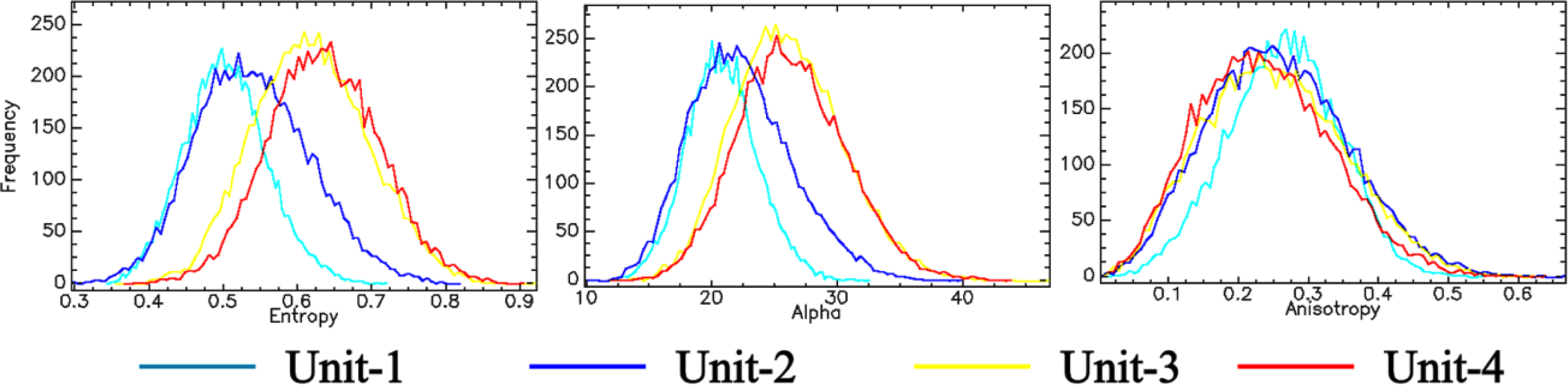
3.3. Scattering Mechanism-Related Parameters of the SRAF

The H/A/α model [31,32] was applied to the RADARSAT-2 full-polarization SAR data collected in the SRAF. Some parameters related to the scattering mechanism were extracted, including the scattering-type angle (α), coherency entropy (H), and anisotropy (A). The distributions of these parameters of the SRAF units of different ages are shown in Figure 6, and the mean values and standard deviation values are listed in

Table 4. The mean values and standard deviation values of the polarimetric parameters and the scattering mechanism-related parameters of the SRAF units (C- and L- designate the C-band and L-band, respectively).

Fan Unit	Scattering Mechanism-Related Parameter			Degree of Polarization				Correlation Coefficient
	Entropy	Alpha	Anisotropy	C-H	C-V	C-R	C-L	HH-VV	RR-LL
Unit-1	0.51 (0.06)	20.9 (2.8)	0.27 (0.08)	0.85 (0.03)	0.89 (0.02)	0.67 (0.06)	0.68 (0.06)	0.77 (0.04)	0.29 (0.08)
Unit-2	0.54 (0.08)	22.4 (4.0)	0.26 (0.10)	0.82 (0.05)	0.86 (0.04)	0.63 (0.09)	0.64 (0.09)	0.76 (0.06)	0.24 (0.10)
Unit-3	0.62 (0.08)	26.2 (4.3)	0.25 (0.10)	0.77 (0.06)	0.82 (0.05)	0.55 (0.10)	0.55 (0.10)	0.7 (0.07)	0.22 (0.10)
Unit-4	0.64 (0.07)	26.5 (4.3)	0.24 (0.09)	0.76 (0.06)	0.8 (0.05)	0.53 (0.10)	0.54 (0.10)	0.7 (0.07)	0.2 (0.10)

.

Based on these results, we can reach the following conclusions: (1) The entropy (H) and scattering-type angle (α) of the SRAF’s units generally follow a decreasing trend with increasing age, which are similar characteristics to those of the backscattering coefficients, and (2) the maximum values occur in the youngest fan unit (Unit-4), whereas the minimum values occur in the oldest fan unit (Unit-1). However, there are some differences found in a comparison between the parameters entropy (H) and scattering-type angle (α) and the backscattering coefficients. The entropy (H) and scattering-type angle (α) of Unit-2 and Unit-3 show relatively clear differences between the two units, whereas the distributions of these parameters are similar in the two younger units (Unit-3 and Unit-4) and in the two older units (Unit-1 and Unit-2). The most plausible explanation for these phenomena includes two principal reasons. One is the obvious bar-and-swale structure on the surfaces of Unit-3 and Unit-4, whereas the surfaces of Unit-1 and Unit-2 are flat and have almost no bar-and-swale structure. Bar-and-swale structures can add complexity to the backscattering return, thus increasing the value of entropy (H) and scattering-type angle (α) parameters. Another reason is that the surfaces of Unit-3 and Unit-4 are sparely covered with dry and low shrubs. The vegetation on the ground also can add the complexity of backscattering return, therefore increasing the value of entropy (H) and scattering-type angle (α) based on Cloude and Pottier’s analyses on these parameters [31,32]. Overall, this surface differences caused by bar-and-swale structure and vegetation may help to explain the differences observed between Units-1, 2 and Units-3, 4. The distribution image of the entropy (H) is shown in Figure 5c as an example, and a blue-red color bar was used to reflect the difference in H. From this figure, the regions with high H, shown as many radiating alluvial channels, cover the regions with low H, indicating the spatial extension characteristics of different geological units.

In contrast with the distributions of entropy (H) and scattering-type angle (α), the distributions of the anisotropy (A) of the four fan units are almost identical and follow a slightly increasing trend with increasing age. Therefore, the anisotropy (A) is not an effective parameter to differentiate the four units of the SRAF.

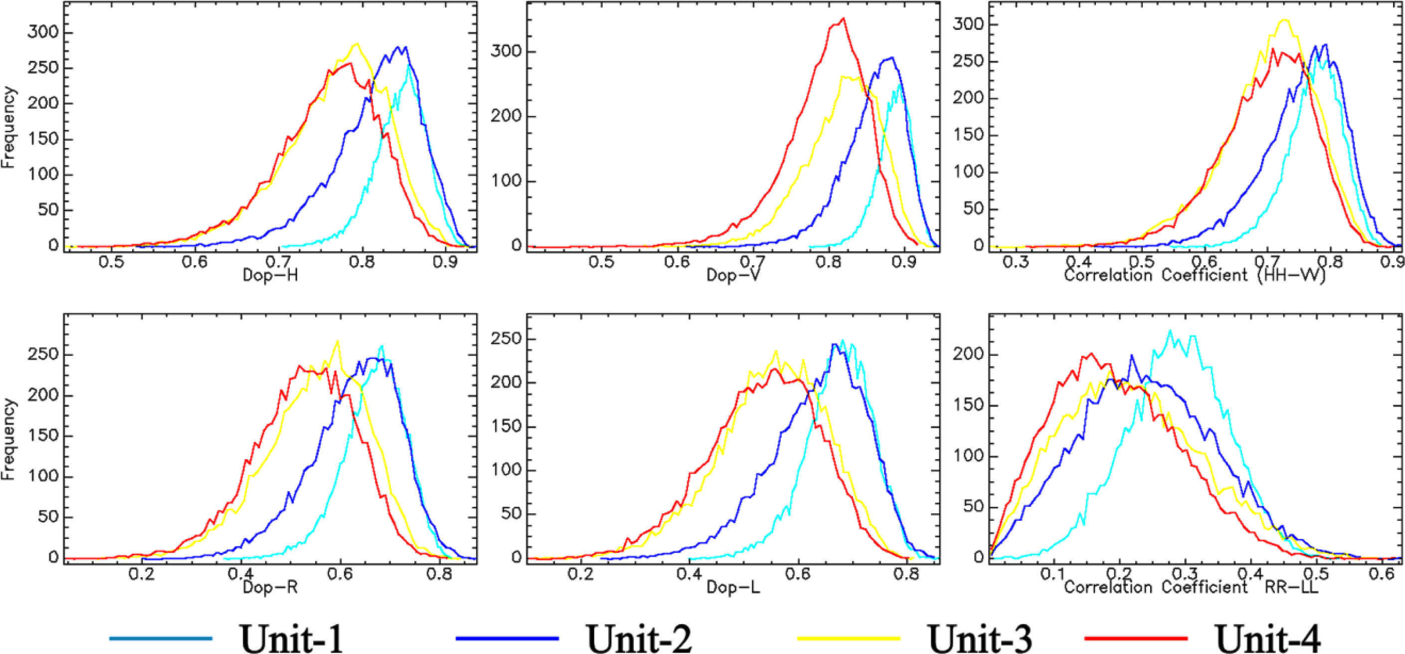
3.4. Polarimetric Parameters of the SRAF

The degree of polarization and the polarimetric correlation coefficient are correlative with the characteristics of the observed targets. The surface of this study area belongs to the distributed target type, or incoherently scattering target type, which usually represent the natural targets. Therefore the polarimetric parameters can be used to describe this surface and they are more sensitive to the geomorphic features in the arid area. The degree of polarization and the correlation coefficient with several typical polarizations of the SRAF were extracted from the RADARSAT-2 C-band polarimetric SAR data. The extracted degrees of polarization include H and V linear polarizations and R and L circular polarizations, and extracted correlation coefficients include the correlation coefficients of the HH-VV and RR-LL polarization states. The results are shown in Figure 7, and the mean values and standard deviation values are listed in Table 4.

Based on these results, the distributions of the degree of polarization and the correlation coefficients in different fan units are similar. Furthermore, with increasing age, the values of these polarimetric parameters generally follow an increasing trend. However, the distribution curves of these parameters are similar, particularly the distributions of the two younger fan units (Unit-3 and Unit-4). Using the degree of polarization of linear H polarization as an example, the curves of the two younger fan units are nearly identical. The values of these curves are lower than those of Unit-1 and Unit-2, indicating a high depolarization effect caused by the clear bar-and-swale structures, the larger gravel size on the surface, and the sparsely distributed vegetation. The distribution images of the degree of polarization of H linear polarization are shown in Figure 5d. Polarimetric parameters can therefore provide additional information to aid in the understanding of the geomorphic features of different fan units and in the mapping of the alluvial fan.

In summary, the backscattering coefficients, scattering mechanism-related parameters, and polarimetric coefficients obtained from SAR data can describe the geomorphic characteristics of an alluvial fan and have the capability to differentiate individual units of an alluvial fan that have different relative ages.

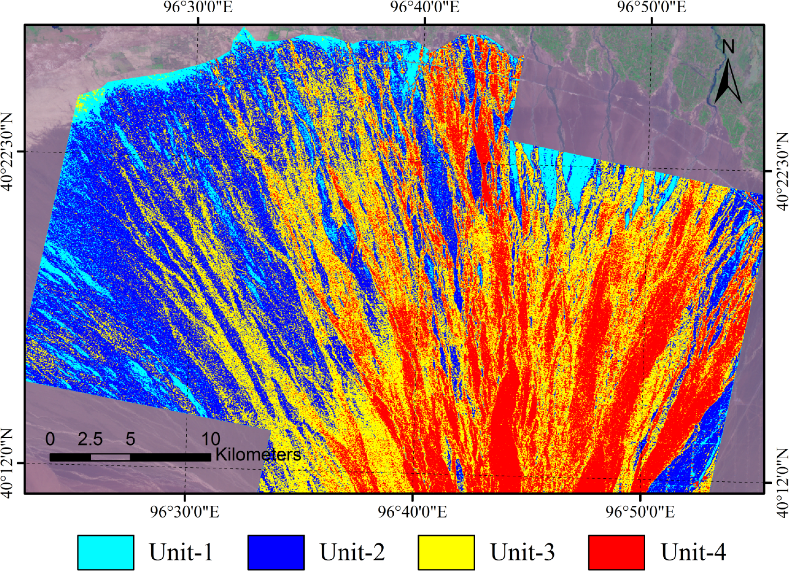
4. Classification of the SRAF Units

The SAR parameters mentioned above can be used to describe the geomorphic features of the surface of an alluvial fan. Using the SRAF as a study area, the SAR parameters that are better adapted to map the fan units of varying ages were selected to carry out the surface classification. These parameters included the C-band backscattering coefficients with HH, HV, VV, RR and LL polarization states, the scattering entropy (H) and scattering-type angle (α).

As seen in Figures 4 and 6, the distributions of these parameters follow an approximately normal distribution. Therefore, the Maximum Likelihood classification method [39,40] can be used to classify the fan units in the SRAF. The Maximum Likelihood classification is a supervised classification based on Bayesian probability and assumes that the statistics for each class in each band are normally distributed. The probability of a given pixel belonging to each of a predefined set of classes is calculated, and the pixel is then assigned to the class for which the probability is the highest.

In this study, the C-band backscattering coefficients with HH, HV, VV, RR, and LL polarization states and the mechanism-related parameters H and α derived from SAR data were selected as an input multiband image for the Maximum Likelihood classifier. Four classes were predefined and they represent the four major fan units of the SRAF (Unit-1, 2, 3, and 4), respectively. Approximately 20,000 pixels near the field survey samples were chosen for each class were chosen as training samples for this classification.

The classification results are shown in Figure 8, indicating the spatial distribution of the four major fan units exposed to the surface. Units 1, 2, 3, and 4 are designated as the colors cyan, blue, yellow, and red, respectively. The gravel size in the heart of the fan is often notably larger than that in other areas because of the powerful transport capacity of the alluvial flows in that region. Therefore, some classification errors can occur in the heart of the fan. As a result, this study concentrates on areas on the fan’s edges.

5. Discussion

Based on the results mentioned above, the temporal-spatial distribution characteristics of the SRAF and the relationship between those characteristics and regional tectonic activities and paleoenvironmental changes are preliminarily discussed in this section. The study surface of the SRAF was covered by four fan units that formed during a time period spanning the later portion of the Late Pleistocene to the Holocene. The spatial distribution of these four units in the SRAF was extracted and is shown in Figure 8, and the temporal information was obtained using the OSL dating technique. A parameter of relative coverage was introduced for a better description of the covering area of a geological unit when it formed in this study, which is defined as a percentage of the covering area of a geological unit estimated form the spatial distribution to the entire study area. The estimated areas of each unit include both the region exposed to the surface and the region covered by the younger fan units. The values of relative coverage of the four units are listed in Table 2.

From Figure 8, most areas of Unit-1, formed at the end of the Late Pleistocene, are covered by the younger fan units, and the rest regions exposed to the surface are located mostly near the edges of the alluvial fan. This pattern indicates that Unit-1 almost covers the entire study area, underlying fan units that formed at an earlier age. Therefore, the relative coverage of Unit-1 was nearly 100%, reflecting an abundant water and sediment supply in this alluvial event. Moreover, the deposit features, such as very small and poorly rounded gravel, nonexistent bar-and-swale morphology, indicate more evenly-distributed, lower energy flow dynamics. The geomorphic features in Unit-2, formed at Middle Holocene, are similar to those of Unit-1. The main differences are that the relative coverage of Unit-2 is 90%, smaller than that of underlying Unit-1, and the gravel size at the surface is larger than that in Unit-1, indicating that the flow is stronger than that in Unit-1.

The OSL dating results indicate that the two younger units (Unit-3 and Unit-4) formed at Late Holocene. The spatial shape of these units is that of many radiating alluvial channels, and the values of relative coverage of Unit-3 and Unit-4 are approximately 50% and 25%, much smaller than those of the older units (Unit-1 and Unit-2), indicating a decrease in water and sediment supply. The deposit features of large size and rounded gravel and developed bar-and-swale pattern reflect increases in stream gradient or stream-energy.

In summary, the main changes in geomorphic features from Unit-1 to Unit-4 include increases in gravel size and roundness, a decrease in spatial extension, and more developed bar-and-swale micro-topography. These changes are attributable to a mechanism of increasing stream-energy and decreasing water and sediment supply. This could be linked to both regional tectonic activities and climate changes. From a tectonics standpoint, the uplift of the Qilian Mountains [34,35] could increase stream gradients and flow velocities. From Figure 8, there appears to be a NW–SE trending offset from Unit-2 to Unit-4. This offset is also a reflection of the uplift of the NanJie Mountain located in the southwest portion of the SRAF. From a climate standpoint, the climate became more arid in Late Holocene, particularly in the Northwest China [36,41,42]. More sporadic and violent rainfall events in this arid period, could contribute to difference between the older units and younger units.

6. Conclusions

Alluvial fans in arid and semi-arid regions can record tectonic and climatic change information. SAR technology, which is sensitive to geomorphic features, plays an important role in quickly mapping alluvial fan units of different ages. The SRAF, the vast alluvial fan located in northwest China, was used as a study area. The application potential of SAR data to the study of alluvial fans is discussed in this paper. Geomorphic features (gravel size, surface roughness, surface desert pavement development, and bar-and-swale structure) and dating samples of four alluvial fan units exposed to the surface were obtained from two field surveys. These units included one unit from the Late Pleistocene, designated as Unit-1, and another three fan units from the Holocene, designated Unit-2, Unit-3, and Unit-4. The dating information was determined by the OSL method.

The RADARSAT-2 C-band full-polarization SAR data and the ALOS-PALSAR L-band dual-polarization SAR data were acquired and used to extract SAR characteristic parameters, including backscattering coefficients, scattering mechanism-related parameters, and several typical polarimetric parameters. In addition, the changes in the characteristics of these SAR parameters in different fan units in the SRAF and the correlation between these SAR parameters and fan units of different ages were studied. Moreover, utilizing these SAR parameters, which are sensitive to differences among the fan units, the spatial distribution of the four alluvial fan units was obtained in the study area by using the Maximum Likelihood classification method. Finally, based on the temporal-spatial distribution characteristics of the SRAF, the changes of these four geological units and their possible links to the regional tectonic activities and climatic changes, combined with the geological survey data, are discussed. Based on our results, we can draw the following conclusions.

(1)

C-band SAR data are more suitable for distinguishing the alluvial fan units of different ages in the SRAF because of the shorter wavelength (5.4 cm) of C-band SAR data compared to that of L-band SAR data (23.6 cm). The most sensitive parameters in this study include the backscattering coefficients with a H-V linear polarization basis and with a R-L circular polarization basis and the scattering mechanism-related parameters entropy (H) and scattering-type angle (α).

(2)

Generally, the backscattering coefficients entropy (H) and scattering-type angle (α) follow a decreasing trend with increasing age. However, there are some differences in this pattern that are caused by differences in surface features, particularly by the existence of a bar-and-swale structure and sparsely distributed vegetation, which is capable of adding to the complexity of the backscattering return.

(3)

SAR data can be used to map the SRAF’s surface during a time period spanning the later portion of the Late Pleistocene to the Holocene, and obtain the temporal-spatial distribution of four alluvial unit (Unit-1,2,3,4), combined with the OSL dating results.

(4)

The main changes in geomorphic features from Unit-1 to Unit-4 include increases in gravel size and roundness, a decrease in spatial extension, and more developed bar-and-swale micro-topography. These changes are attributable to a mechanism of increasing stream-energy and decreasing water and sediment supply. This could be linked to both regional tectonic activities and paleoenvironmental changes. As a result, SAR data can provide valuable information for tectonic and paleoenvironmental research of the SRAF area.

References and Notes

1. Dorn, R.I. The Role of Climatic Change in Alluvial Fan Development. In Geomorphology of Desert Environments, 2nd ed; Parsons, A.J., Abrahams, A.D., Eds.; Springer: Dordrecht, The Netherlands, 2009; pp. 723–742. [Google Scholar]
2. Nichols, K.K.; Bierman, P.R.; Foniri, W.R.; Gillespie, A.R.; Caffee, M.; Finkel, R. Dates and rates of arid region geomorphic processes. GSA Today 2006, 16, 4–11. [Google Scholar]
3. Bull, W.B. Geomorphic Responses to Climatic Change; Oxford University Press: New York, NY, USA, 1991. [Google Scholar]
4. Birkeland, P.W. Soils and Geomorphology; Oxford University Press: New York, NY, USA, 1984. [Google Scholar]
5. Bull, W.B. The alluvial-fan environment. Prog. Phys. Geog 1977, 1, 222–270. [Google Scholar]
6. Kiss, T.; Sümeghy, B.; Sipos, G. Late Quaternary paleodrainage reconstruction of the Maros River alluvial fan. Geomorphology 2014, 204, 49–60. [Google Scholar]
7. Gómez-Paccard, M.; López-Blanco, M.; Costa, E.; Garcés, M.; Beamud, E.; Larrasoańa, J.C. Tectonic and climatic controls on the sequential arrangement of an alluvial fan/fan-delta complex (Montserrat, Eocene, Ebro Basin, NE Spain). Basin Res 2012, 24, 437–455. [Google Scholar]
8. Macklin, M.G.; Lewin, J.; Woodward, J.C. The fluvial record of climate change. Phil. Trans. R. Soc. A 2012, 370, 2143–2172. [Google Scholar]
9. Wells, S.G.; McFadden, L.D.; Dohrenwend, J.C. Influence of late Quaternary climatic changes on geomorphic and pedogenic processes on a desert piedmont, Eastern Mojave Desert, California. Quat. Res 1987, 27, 130–146. [Google Scholar]
10. McFadden, L.D.; Ritter, J.B.; Wells, S.G. Use of multiparameter relative-age methods for age estimation and correlation of alluvial fan surfaces on a desert piedmont, eastern Mojave Desert, California. Quat. Res 1989, 32, 276–290. [Google Scholar]
11. Guo, H. Radar Earth Observation Theory and Applications; (in Chinese); Science Press: Beijing, China, 2000. [Google Scholar]
12. Zani, H.; Assine, M.L.; McGlue, M.M. Remote sensing analysis of depositional landforms in alluvial settings: Method development and application to the Taquari megafan, Pantanal (Brazil). Geomorphology 2012, 161–162, 82–92. [Google Scholar]
13. Ferrier, G.; Pope, R.J.J. Quantitative mapping of alluvial fan evolution using ground-based reflectance spectroscopy. Geomorphology 2012, 175–176, 14–24. [Google Scholar]
14. Le Page, M.; Berjamy, B.; Fakir, Y.; Bourgin, F.; Jarlan, L.; Abourida, A.; Benrhanem, M.; Jacob, G.; Huber, M.; Sghrer, F.; et al. An integrated DSS for groundwater management based on remote sensing. The case of a semi-arid aquifer in Morocco. Water Resour. Manag 2012, 26, 3209–3230. [Google Scholar]
15. Farr, T.G.; Chadwick, O.A. Geomorphic processes and remote sensing signatures of alluvial fans in the Kun Lun mountains, China. J. Geophys. Res 1996, 101, 23091–23100. [Google Scholar]
16. Kierein-Young, K.S. The integration of optical and radar data to characterize mineralogy and morphology of surfaces in Death Valley, California, USA. Int. J. Remote Sens 1997, 18, 1517–1541. [Google Scholar]
17. Wang, C.; Guo, H. Estimation of surface parameters from polarimetric SIR-C data (in Chinese). J. Remote Sens 1998, 2, 107–111. [Google Scholar]
18. Liao, J.; Pang, Z. Surface Parameters Retrieval from Alluvial Fan in Ejina Area of Inner Mongolia Using Multi-polarization SAR Data. Proceedings of the IEEE International on Geoscience and Remote Sensing Symposium, IGARSS 2009, Cape Town, South Africa, 12–17 July 2009.
19. Duarte, M.R.; Wozniak, E.; Recondo, C.; Cabo, C.; Marquínez, J.; Fernández, S. Estimation of surface roughness and stone cover in burnt soils using SAR images. Catena 2008, 74, 264–272. [Google Scholar]
20. Zhang, L.; Guo, H.; Liao, J.; Han, C. Research on copolarized correlation characteristic from Bodunqi alluvial fan using full-polarized SAR data (in Chinese). Remote Sens. Technol. Appl 2008, 23, 385–388. [Google Scholar]
21. Hung, W.-C.; Hwang, C.; Chen, Y.-A.; Chang, C.-P.; Yen, J.-Y.; Hooper, A.; Yang, C.-Y. Surface deformation from persistent scatterers SAR interferometry and fusion with leveling data: A case study over the Choushui River Alluvial Fan, Taiwan. Remote Sens. Environ 2011, 115, 957–967. [Google Scholar]
22. Catalano, S.; Bonforte, A.; Guglielmino, F.; Romagnoli, G.; Tarsia, C.; Tortorici, G. The influence of erosional processes on the visibility of Permanent Scatterers Features from SAR remote sensing on Mount Etna (E Sicily). Geomorphology 2013, 198, 128–137. [Google Scholar]
23. Zhang, L.; Liao, J.J.; Guo, H.D.; Han, C.M. Retrieving surface characteristic of alluvial fan from shuttle imaging radar data based on genetic algorithm and backscattering model (in Chinese). Chin. High Technol. Letters 2008, 8, 851–856. [Google Scholar]
24. Oh, Y.; Sarabandi, K.; Ulaby, F.T. Semi-empirical model of the ensemble-averaged differential mueller matrix for microwave backscattering from bare soil surfaces. IEEE Trans. Geosci. Remote Sens 2002, 40, 1348–1355. [Google Scholar]
25. Oh, Y.; Sarabandi, K.; Ulaby, F.T. An empirical model and an inversion technique for radar scattering from bare soil surfaces. IEEE Trans. Geosci. Remote Sens 1992, 30, 370–381. [Google Scholar]
26. Moreira, A.; Prats-Iraola, P.; Younis, M.; Krieger, G.; Hajnsek, I.; Papathanassiou, K.P. A tutorial on synthetic aperture radar. IEEE Geosci. Remote Sens. Mag 2013, 1, 6–43. [Google Scholar]
27. Werninghaus, R.; Buckreuss, S. The TerraSAR-X mission and system design. IEEE Trans. Geosci. Remote Sens 2010, 48, 606–614. [Google Scholar]
28. Morena, L.C.; James, K.V.; Beck, J. An introduction to the RADARSAT-2 mission. Can. J. Remote Sens 2004, 30, 221–234. [Google Scholar]
29. Rosenqvist, A.; Shimada, M.; Ito, N.; Watanabe, M. ALOS PALSAR: A pathfinder mission for global-scale monitoring of the environment. IEEE Trans. Geosci. Remote Sens 2007, 45, 3307–3316. [Google Scholar]
30. Guo, H.; Li, X. Technical characteristics and potential application of the new generation SAR for earth observation (in Chinese). Chin. Sci. Bull 2011, 56, 1155–1168. [Google Scholar]
31. Cloude, S.R.; Pottier, E. An entropy based classification scheme for land applications of polarimetric SAR. IEEE Trans. Geosci. Remote Sens 1997, 35, 68–78. [Google Scholar]
32. Cloude, S.R.; Pottier, E. A review of target decomposition theorems in radar polarimetry. IEEE Trans. Geosci. Remote Sens 1996, 34, 498–518. [Google Scholar]
33. Freeman, A.; Durden, S.L. A three-component scattering model for polarimetric SAR data. IEEE Trans. Geosci. Remote Sens 1998, 36, 963–973. [Google Scholar]
34. Wang, P.; Lu, Y.; Ding, G.; Chen, J.; Karl, H.W. Response of the development of the Shule River alluvial fan to tectonic activity. Quat. Sci. 2004, 24, 74–81. [Google Scholar]
35. Wang, P. Development of the Shule Alluvial-Fan and its Response to Tectonic Activity in Gansu Province, China—Characteristics of Neotectonic Activity of the East End of the Altyn Tagh Fault (in Chinese). Institute of Geology, China Earthquake Administration, Beijing, China, 2003. [Google Scholar]
36. Mao, H.; Zhao, H.; Lu, Y.; Wang, C.; Zhang, K.; Yang, Z.; Liang, J. Pollen assemblages and environment evolution in shule river alluvial fan oasis of Gansu Province in Holocene. ACTA Geosci. Sin 2007, 28, 528–534. [Google Scholar]
37. Huntley, D.J.; Godfrey-Smith, D.I.; Thewalt, M.L.W. Optical dating of sediments. Nature 1985, 313, 105–107. [Google Scholar]
38. Jong-Sen, L.; Pottier, E. Polarimetric Radar Imaging: From Basics to Applications; CRC Press: Boca Raton, FL, USA, 2009. [Google Scholar]
39. Richard, J.A.; Jia, X. Remote Sensing Digital Image Analysis: An Introduction, 3rd ed; Springer: Berlin, Germany, 1999. [Google Scholar]
40. Mather, P.; Tso, B. Classification Methods for Remotely Sensed Data; CRC Press: Boca Raton, FL, USA, 2010. [Google Scholar]
41. Yao, T.; Thompson, L.G.; Shi, Y.; Qin, D.; Jiao, K.; Yang, Z.; Tian, L.; Thompson, E.M. Climate variation since the Last Interglaciation recorded in the Guliya ice core. Sci. China Ser. D: Earth Sci 1997, 40, 662–668. [Google Scholar]
42. Wu, Y.; Yang, T.; Yu, Y.; Liu, X.; An, C.; Li, Y.; Su, X. Holocene climate change and the ancient culture response in central Hexi corridor (in Chinese). Arid Zone Res 2006, 23, 650–653. [Google Scholar]
Figure 1. The location of the SRAF. The background is the RGB pseudo-color image from a LandSat TM image (Red: band-7, Green: band-4, Blue: band-1). The footprints of the RADARSAT-2 and ALOS-PALSAR SAR dataset collected in this area are shown as red and blue rectangles, respectively.
Remotesensing 05 06997f1
Figure 2. The (RGB) pseudo-color composite images of SAR data of the SRAF (a) ALOS-PALSAR dual-polarization SAR data (R: HV, G: HH − HV, B: HH). (b) RADARSAT-2 full-polarization SAR data (R: HH-VV, G: 2HV, B: HH + VV).
Remotesensing 05 06997f2
Figure 3. Photographs of the SRAF’s four surface units. (a) Unit-1 (∼11.3 ka). (b) Unit-2 (∼5.6 ka). (c) Unit-3 (∼1.0 ka). (d) Unit-4 (∼0.5 ka).
Remotesensing 05 06997f3
Figure 4. The distribution characteristics of the SRAF units’ backscattering coefficients with different channels, including the C-HH, C-VV, C-HV, C-RR, C-LL, C-RL, L-HH, and L-HV channels.
Remotesensing 05 06997f4
Figure 5. The distributions of parameters from the SAR image, including (a) the backscattering coefficient of HV; (b) the backscattering coefficient of RR; (c) the entropy; and (d) the degree of polarization of V polarization.
Remotesensing 05 06997f5
Figure 6. The distribution characteristics of the scattering mechanism-related parameters, including entropy (H), anisotropy (A) and scattering type angle (α), in the different SRAF units.
Remotesensing 05 06997f6
Figure 7. The distribution characteristics of the degree of polarization (C-H, C-V, C-R, C-L polarizations) and of the correlation coefficient (HH-VV, RR-LL).
Remotesensing 05 06997f7
Figure 8. The spatial distributions of fan units in the SRAF.
Remotesensing 05 06997f8