Long-Term Satellite Detection of Post-Fire Vegetation Trends in Boreal Forests of China


Abstract
:
1. Introduction
2. Data and Method
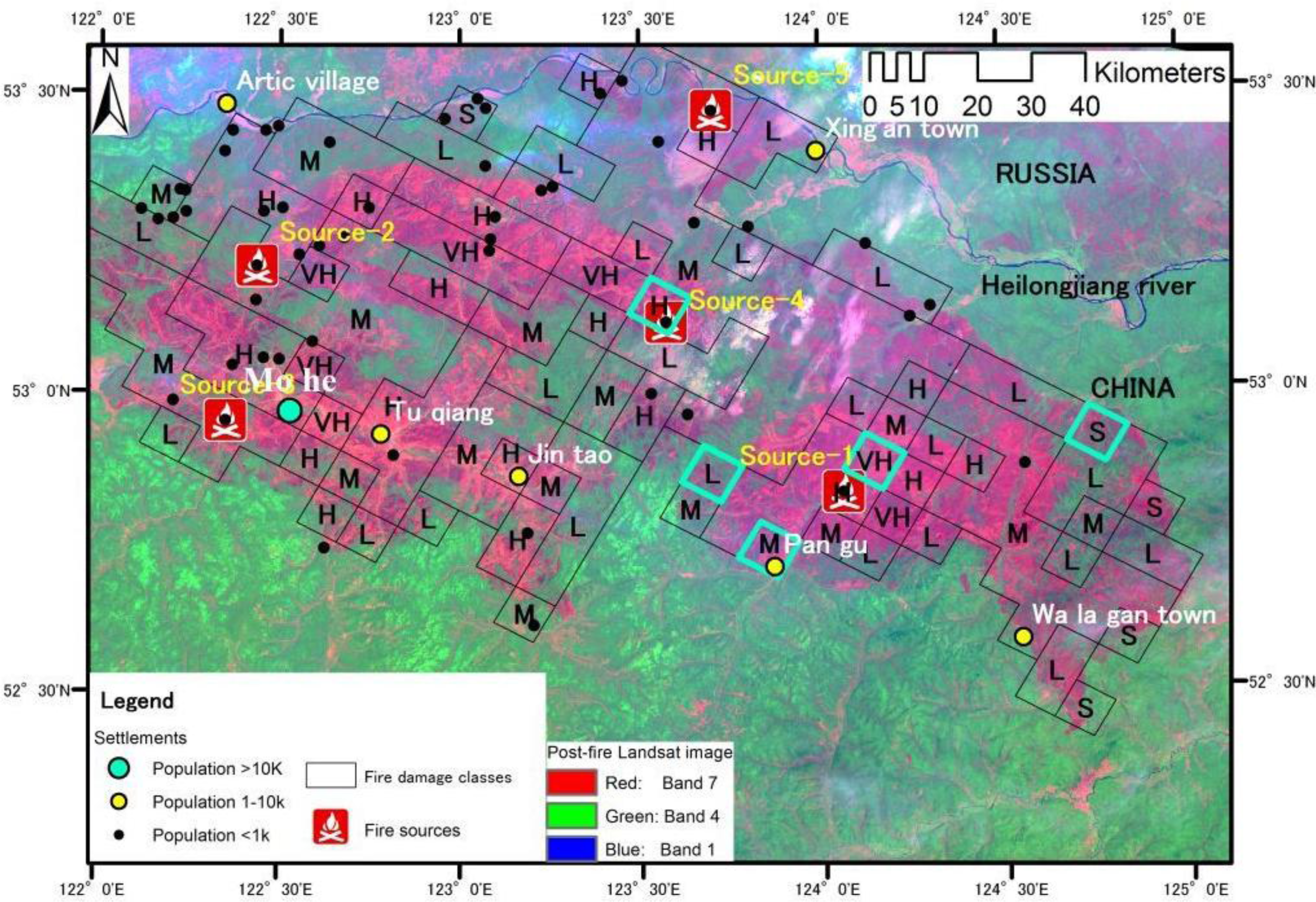
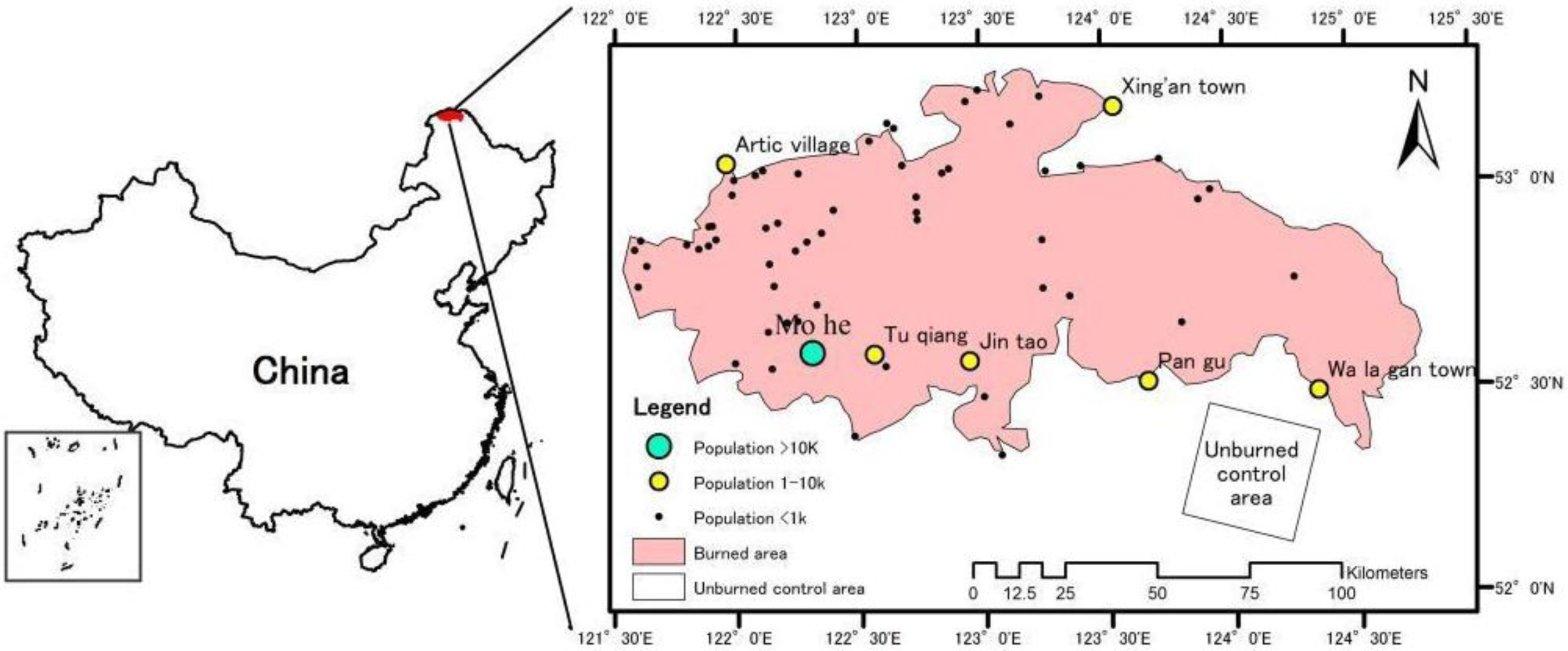
2.1. Study Area
2.2. Data
2.2.1. AVHRR GIMMS 15-Day Composite NDVI Dataset
2.2.2. Landsat Imagery
2.3. Method
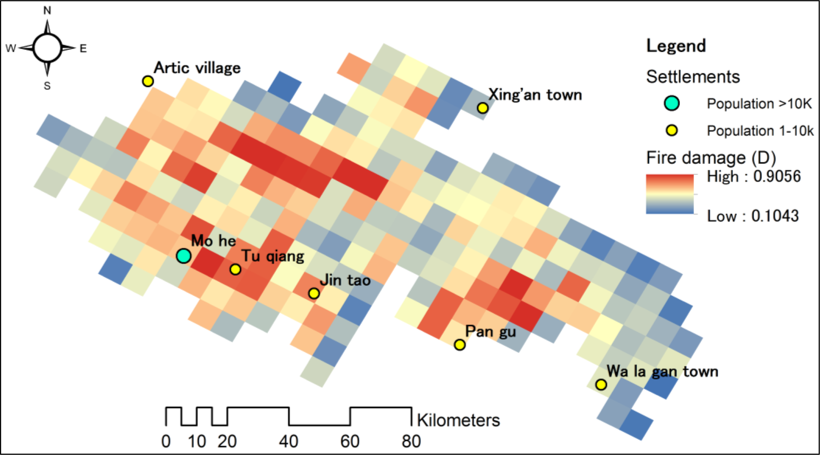
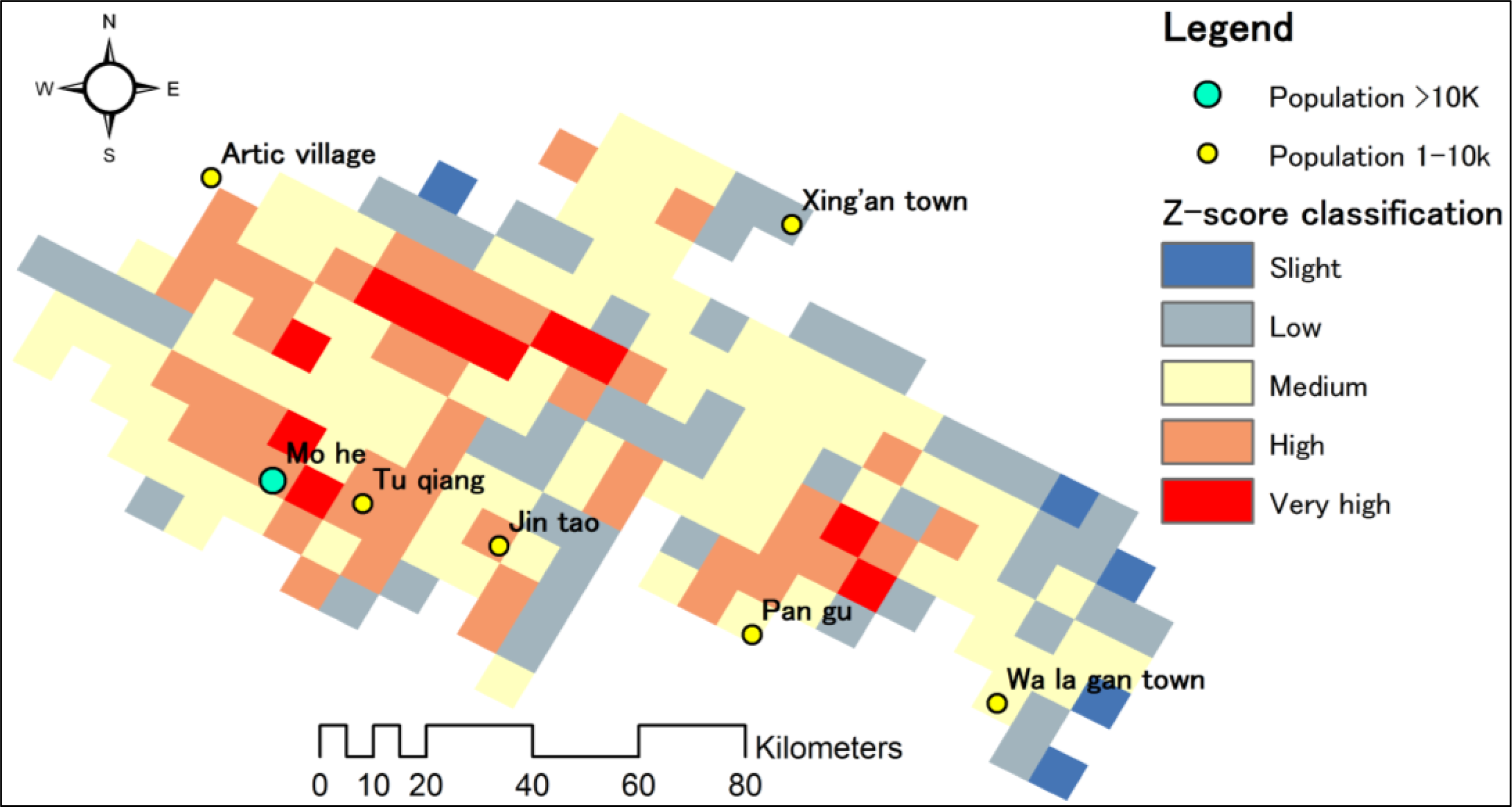
2.3.1. Mapping Fire Damage
2.3.2. Modeling of Vegetation Recovery
2.3.3. Mann-Kendall Trend Assessment
3. Results and Discussion
3.1. Fire Damage Assessment
3.2. Temporal Analysis of Post-Fire Vegetation Trajectory
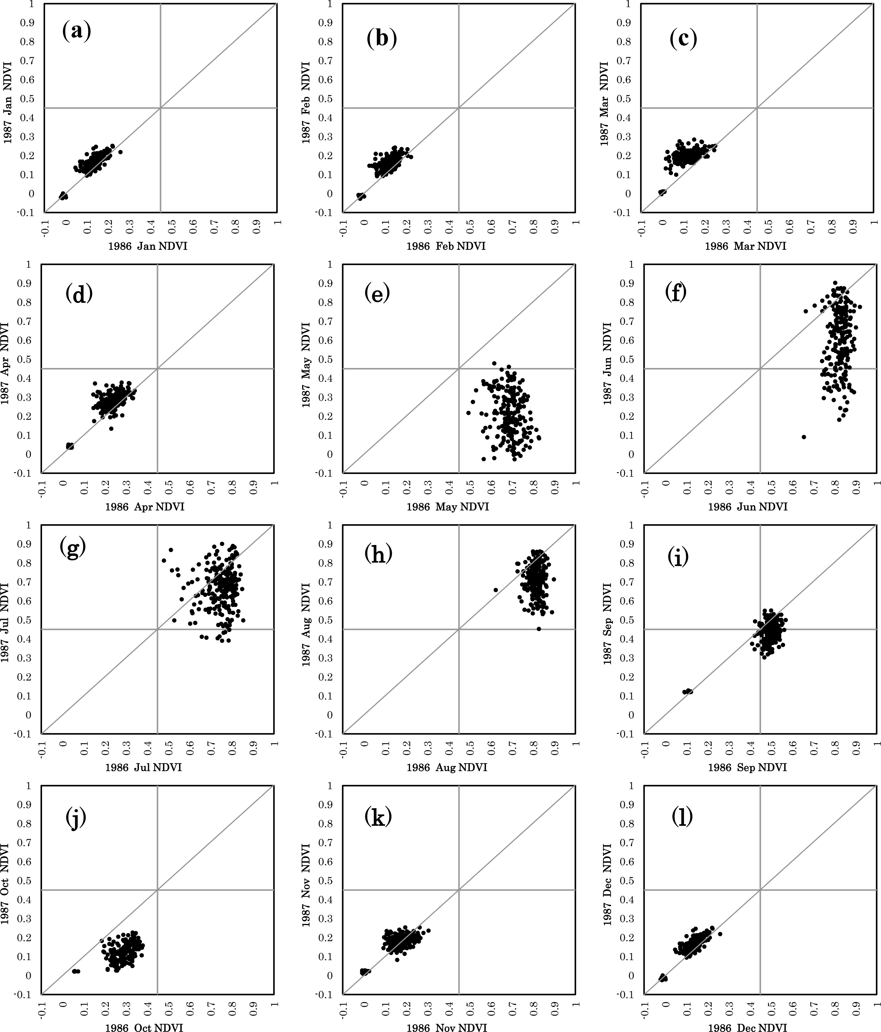
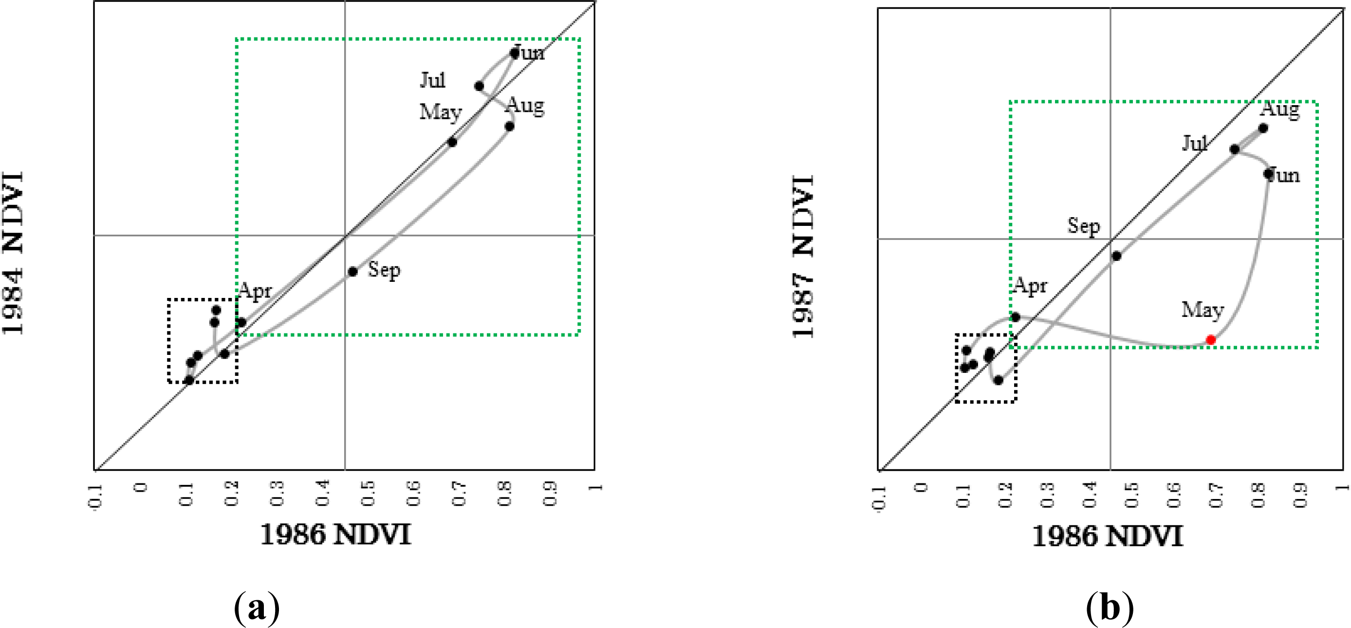
3.2.1. Monthly Dynamics of Post-Fire Vegetation Trajectory
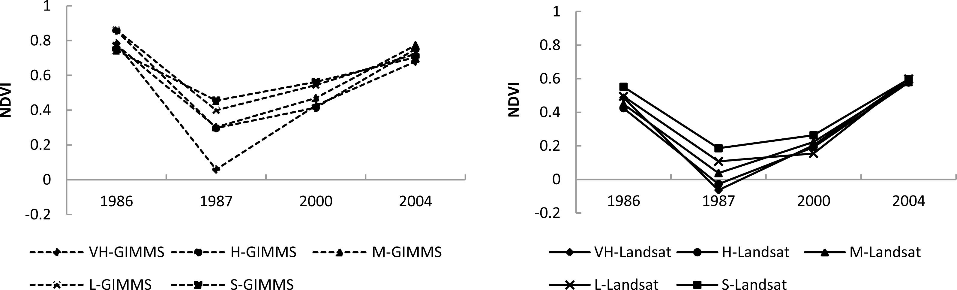
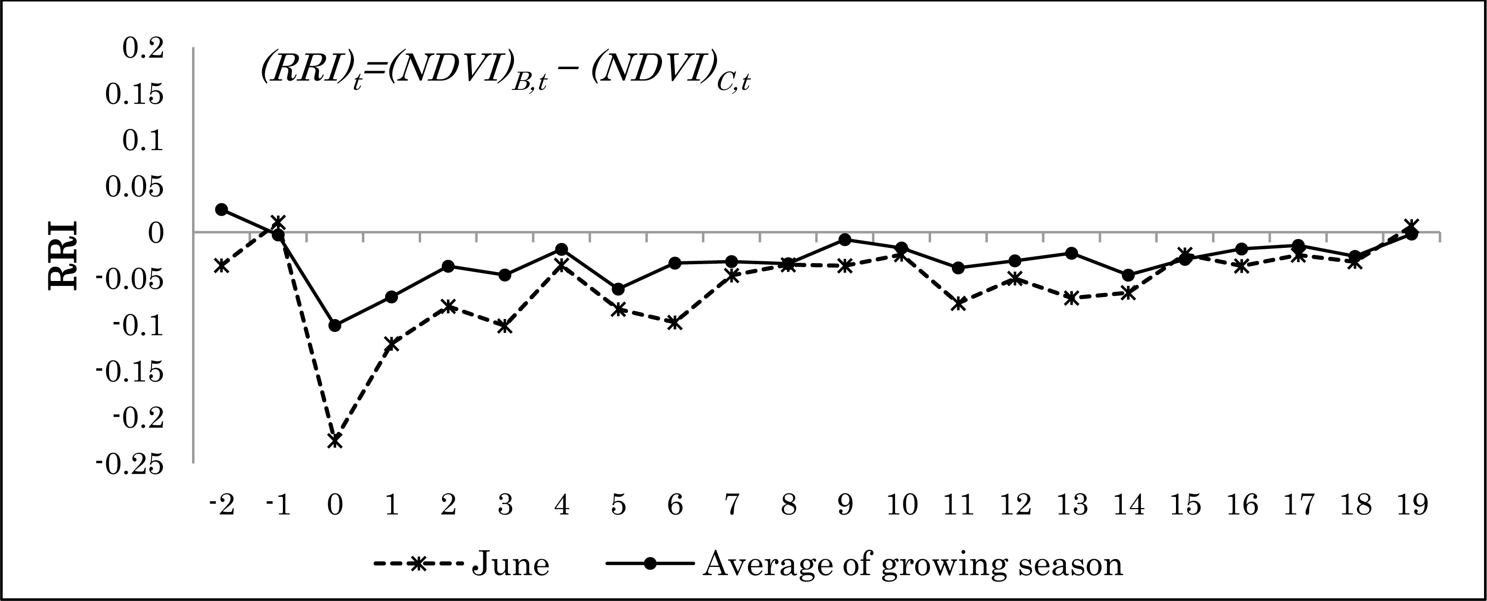
3.2.2. Yearly Dynamics of Post-Fire Vegetation
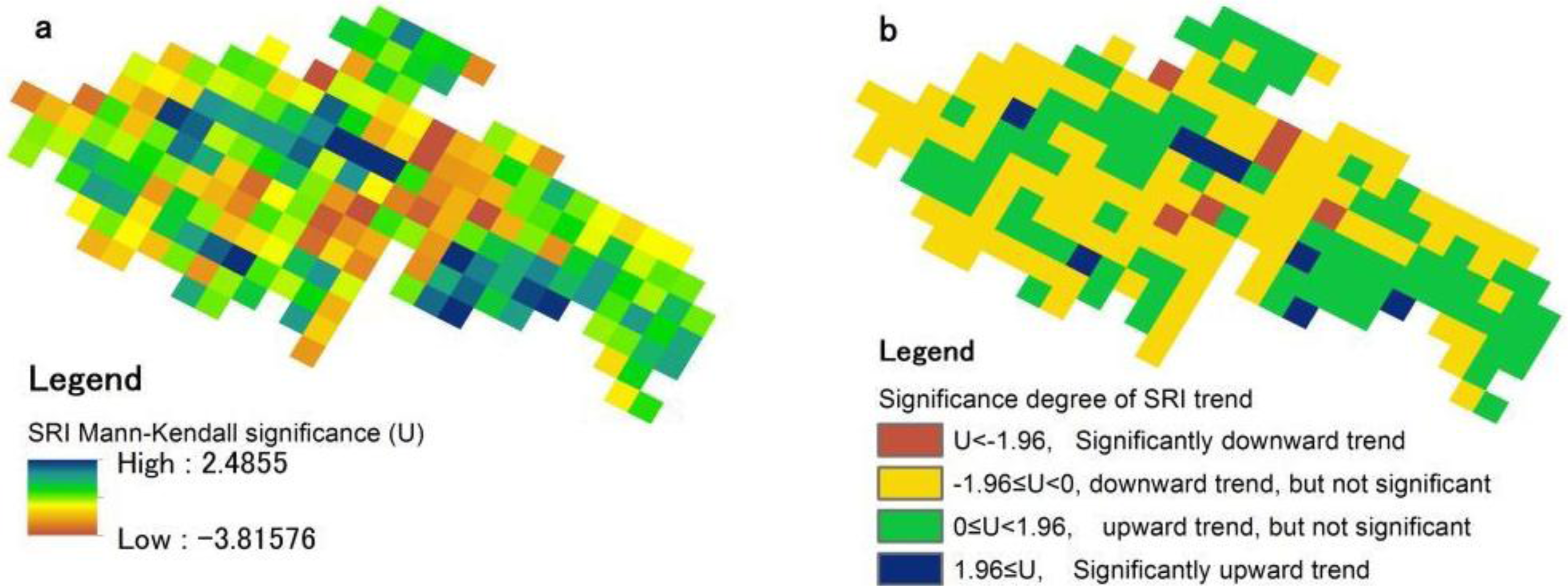
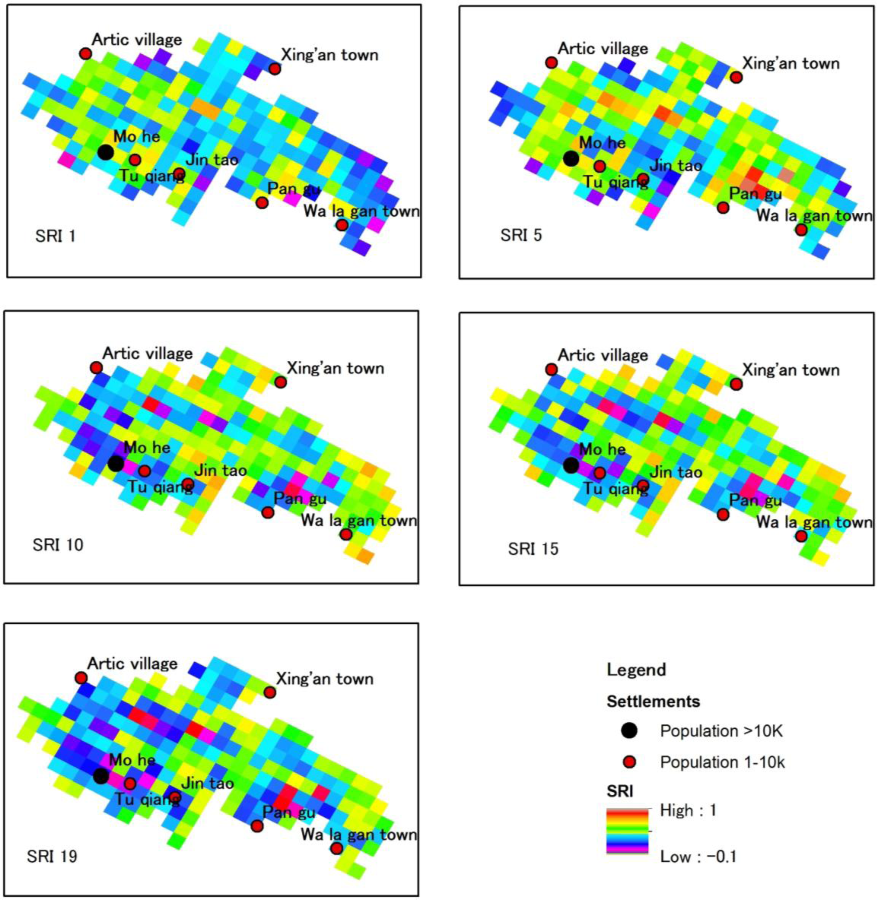
3.3. Spatial Pattern and Trend Analysis of Post-Fire Stands Regrowth Index (SRI)
3.4. Assessment against Landsat-NDVI
4. Conclusion
Acknowledgments
Conflicts of Interest
Reference
- Beck, P.S.A.; Goetz, S.J.; Mack, M.C.; Alexander, H.D.; Jin, Y.; Randerson, J.T.; Loranty, M.M. The impacts and implications of an intensifying fire regime on Alaskan boreal forest composition and albedo. Glob. Chang. Biol 2011, 17, 2853–2866. [Google Scholar]
- Wulder, M.A.; White, J.C.; Alvarez, F.; Han, T.; Rogan, J.; Hawkes, B. Characterizing boreal forest wildfire with multi-temporal Landsat and Lidar data. Remote Sens. Environ 2009, 113, 1540–1555. [Google Scholar]
- Kang, S.; Kimball, J.S.; Running, S.W. Simulating effects of fire disturbance and climate change on boreal forest productivity and evapotranspiration. Sci. Total Environ 2006, 362, 85–102. [Google Scholar]
- Cahoon, D.R.; Stocks, B.J.; Levine, J.S.; Cofer, W.R.; Pierson, J.M. Satellite analysis of the severe 1987 forest fires in northern China and southeastern Siberia. J. Geophys. Res.: Atmos 1994, 99, 18627–18638. [Google Scholar]
- Tan, K.; Piao, S.; Peng, C.; Fang, J. Satellite-based estimation of biomass carbon stocks for northeast China’s forests between 1982 and 1999. For. Ecol. Manag 2007, 240, 114–121. [Google Scholar]
- Fang, J.; Chen, A.; Peng, C.; Zhao, S.; Ci, L. Changes in forest biomass carbon storage in China between 1949 and 1998. Science 2001, 292, 2320–2322. [Google Scholar]
- Zhong, M.; Fan, W.; Liu, T.; Li, P. Statistical analysis on current status of China forest fire safety. Fire Saf. J 2003, 38, 257–269. [Google Scholar]
- Goetz, S.J.; Fiske, G.J.; Bunn, A.G. Using satellite time-series data sets to analyze fire disturbance and forest recovery across Canada. Remote Sens. Environ 2006, 101, 352–365. [Google Scholar]
- Cuevas-GonzÁLez, M.; Gerard, F.; Balzter, H.; RiaÑO, D. Analysing forest recovery after wildfire disturbance in boreal Siberia using remotely sensed vegetation indices. Glob. Chang. Biol 2009, 15, 561–577. [Google Scholar]
- Matthews, S.; Sullivan, A.; Gould, J.; Hurley, R.; Ellis, P.; Larmour, J. Field evaluation of two image-based wildland fire detection systems. Fire Saf. J 2012, 47, 54–61. [Google Scholar]
- Segah, H.; Tani, H.; Hirano, T. Detection of fire impact and vegetation recovery over tropical peat swamp forest by satellite data and ground-based NDVI instrument. Int. J. Remote Sens 2010, 31, 5297–5314. [Google Scholar]
- Parsons, A. Burned Area Emergency Rehabilitation Soil Burn Severity Definitions and Mapping Guidelines Draft; USDA Forest Service, Rocky Mountain Research Station: Missoula, MT, USA, 2003. [Google Scholar]
- Balzter, H.; Gonzalez, M.C.; Gerard, F.; Riaño, D. Post-Fire Vegetation Phenology in Siberian Burn Scars. Proceedings of 2007 IEEE International Geoscience and Remote Sensing Symposium, Barcelona, Spain, 23–28 July 2007; pp. 4652–4655.
- Telesca, L.; Lasaponara, R. Pre- and post-fire behavioral trends revealed in satellite NDVI time series. Geophys. Res. Lett. 2006, 33. [Google Scholar] [CrossRef]
- Leon, J.R.R.; van Leeuwen, W.J.D.; Casady, G.M. Using MODIS-NDVI for the modeling of post-wildfire vegetation response as a function of environmental conditions and pre-fire restoration treatments. Remote Sens 2012, 4, 598–621. [Google Scholar]
- Zhou, L.M.; Tucker, C.J.; Kaufmann, R.K.; Slayback, D.; Shabanov, N.V.; Myneni, R.B. Variations in northern vegetation activity inferred from satellite data of vegetation index during 1981 to 1999. J. Geophys. Res.: Atmos 2001, 106, 20069–20083. [Google Scholar]
- Wang, X.; He, H.S.; Li, X. The long-term effects of fire suppression and reforestation on a forest landscape in Northeastern China after a catastrophic wildfire. Landsc. Urban Plan 2007, 79, 84–95. [Google Scholar]
- Wu, Z.W.; He, H.S.; Chang, Y.; Liu, Z.H.; Chen, H.W. Development of customized fire behavior fuel models for boreal forests of northeastern China. Environ. Manag 2011, 48, 1148–1157. [Google Scholar]
- Turner, M.G.; Romme, W.H.; Gardner, R.H.; Hargrove, W.W. Effects of fire size and pattern on early succession in Yellowstone National Park. Ecol. Monogr 1997, 67, 411–433. [Google Scholar]
- Li, X.; He, H.S.; Wu, Z.; Liang, Y.; Schneiderman, J.E. Comparing effects of climate warming, fire, and timber harvesting on a boreal forest landscape in northeastern China. PLoS One 2013, 8, e59747. [Google Scholar]
- Pouliot, D.; Latifovic, R.; Olthof, I. Trends in vegetation NDVI from 1 km AVHRR data over Canada for the period 1985–2006. Int. J. Remote Sens 2009, 30, 149–168. [Google Scholar]
- Bastos, A.; Gouveia, C.M.; DaCamara, C.C.; Trigo, R.M. Modelling post-fire vegetation recovery in Portugal. Biogeosciences 2011, 8, 3593–3607. [Google Scholar]
- Viedma, O.; Melia, J.; Segarra, D.; GarciaHaro, J. Modeling rates of ecosystem recovery after fires by using Landsat TM data. Remote Sens. Environ 1997, 61, 383–398. [Google Scholar]
- Van Leeuwen, W.J.D. Monitoring the effects of forest restoration treatments on post-fire vegetation recovery with MODIS multitemporal data. Sensors 2008, 8, 2017–2042. [Google Scholar]
- Kennedy, R.E.; Yang, Z.; Cohen, W.B.; Pfaff, E.; Braaten, J.; Nelson, P. Spatial and temporal patterns of forest disturbance and regrowth within the area of the Northwest Forest Plan. Remote Sens. Environ 2012, 122, 117–133. [Google Scholar]
- Gouveia, C.; DaCamara, C.C.; Trigo, R.M. Post-fire vegetation recovery in Portugal based\newline on spot/vegetation data. Nat. Hazard. Earth Syst. Sci 2010, 10, 673–684. [Google Scholar]
- Hope, A.; Albers, N.; Bart, R. Characterizing post-fire recovery of fynbos vegetation in the Western Cape Region of South Africa using MODIS data. Int. J. Remote Sens 2012, 33, 979–999. [Google Scholar]
- Lampainen, J.; Kuuluvainen, T.; Wallenius, T.H.; Karjalainen, L.; Vanha-Majamaa, I. Long-term forest structure and regeneration after wildfire in Russian Karelia. J. Veg. Sci 2004, 15, 245–256. [Google Scholar]
- Mann, H.B. Nonparametric tests against trend. Econometrica 1945, 13, 245–259. [Google Scholar]
- Kendall, M.G. Rank Correlation Methods; Griffin: London, UK, 1975. [Google Scholar]
- Neeti, N.; Eastman, J.R. A contextual mann-kendall approach for the assessment of trend significance in image time series. Trans. GIS 2011, 15, 599–611. [Google Scholar]
- Lee, S.-W.; Lee, M.-B.; Lee, Y.-G.; Won, M.-S.; Kim, J.-J.; Hong, S.-K. Relationship between landscape structure and burn severity at the landscape and class levels in Samchuck, South Korea. For. Ecol. Manag 2009, 258, 1594–1604. [Google Scholar]
- Nielsen, E.M.; Prince, S.D.; Koeln, G.T. Wetland change mapping for the US mid-Atlantic region using an outlier detection technique. Remote Sens. Environ 2008, 112, 4061–4074. [Google Scholar]
- Veraverbeke, S.; Gitas, I.; Katagis, T.; Polychronaki, A.; Somers, B.; Goossens, R. Assessing post-fire vegetation recovery using red-near infrared vegetation indices: Accounting for background and vegetation variability. ISPRS J. Photogramm. Remote Sens 2012, 68, 28–39. [Google Scholar]
- Pausas, J.G.; Bradstock, R.A.; Keith, D.A.; Keeley, J.E.; Network, G.F. Plant functional traits in relation to fire in crown-fire ecosystems. Ecology 2004, 85, 1085–1100. [Google Scholar]
- Li, X.; He, H.; Wang, X.; Xie, F.; Hu, Y.; Li, Y. Tree planting: How fast can it accelerate post-fire forest restoration?—A case study in Northern Da Hinggan Mountains, China. Chin. Geogr. Sci 2010, 20, 481–490. [Google Scholar]
- Wang, X.; He, H.S.; Li, X.; Chang, Y.; Hu, Y.; Xu, C.; Bu, R.; Xie, F. Simulating the effects of reforestation on a large catastrophic fire burned landscape in Northeastern China. For. Ecol. Manag 2006, 225, 82–93. [Google Scholar]
- Wang, J.; Meng, J.J.; Cai, Y.L. Assessing vegetation dynamics impacted by climate change in the southwestern karst region of China with AVHRR NDVI and AVHRR NPP time-series. Environ. Geol 2008, 54, 1185–1195. [Google Scholar]
- Tucker, C.J.; Pinzon, J.E.; Brown, M.E.; Slayback, D.A.; Pak, E.W.; Mahoney, R.; Vermote, E.F.; El Saleous, N. An extended AVHRR 8-km NDVI dataset compatible with MODIS and SPOT vegetation NDVI data. Int. J. Remote Sens 2005, 26, 4485–4498. [Google Scholar]
- Fensholt, R.; Sandholt, I.; Stisen, S.; Tucker, C. Analysing NDVI for the African continent using the geostationary meteosat second generation SEVIRI sensor. Remote Sens. Environ 2006, 101, 212–229. [Google Scholar]
- Anyamba, A.; Tucker, C.J. Analysis of Sahelian vegetation dynamics using NOAA-AVHRR NDVI data from 1981–2003. J. Arid Environ 2005, 63, 596–614. [Google Scholar]
- Shoshany, M.; Karnibad, L. Mapping shrubland biomass along Mediterranean climatic gradients: The synergy of rainfall-based and NDVI-based models. Int. J. Remote Sens 2011, 32, 9497–9508. [Google Scholar]
- Santin-Janin, H.; Garel, M.; Chapuis, J.L.; Pontier, D. Assessing the performance of NDVI as a proxy for plant biomass using non-linear models: A case study on the Kerguelen archipelago. Polar Biol 2009, 32, 861–871. [Google Scholar]


| Year | Date | Sensor | Path/Row |
|---|---|---|---|
| 1986 | 5 June | TM | 121/23 |
| 1987 | 24 June | TM | 121/23 |
| 1987 | 15 June | TM | 121/22 |
| 2000 | 19 June | ETM+ | 121/23 |
| 2004 | 22 June | TM | 121/23 |
| Pre-Fire Year (1984–1986) | Post-Fire Year (1987) | Standard Difference | z-Score | Fire Damage Class | Pixels | Percentage (%) |
|---|---|---|---|---|---|---|
| 0.7708 | 0.6542 | −2∼−1 | 1 | Slight | 5 | 2.44% |
| 0.7764 | 0.5352 | −1∼0 | 2 | Low | 49 | 23.90% |
| 0.7852 | 0.3868 | 0∼1 | 3 | Medium | 94 | 45.85% |
| 0.7884 | 0.2239 | 1∼2 | 4 | High | 46 | 22.44% |
| 0.8165 | 0.0524 | 2∼999 | 5 | Very high | 11 | 5.37% |
| Fire Source | Name | Longitude | Latitude | Burned Area | Ignition Reason |
|---|---|---|---|---|---|
| Source-1 | Gulian | 122°22′ | 52°26′ | 38 × 104 ha | Electric spark |
| Source-2 | Hewan | 122°21′ | 53°11′ | 33.8 × 10⁴ ha | Smoking |
| Source-3 | Pangu | 123°43′ | 52°45′ | 28 × 104 ha | Unknown |
| Source-4 | Xingan | 122°22′ | 122°22′ | 616 ha | Smoking |
| Source-5 | Yixi | 123°25′ | 53°05′ | 587 ha | Electric spark |
| Fire Damage Class | Mann-Kendal Significance (U) | ||||
|---|---|---|---|---|---|
| U < −1.96 | −1.96 ≤ U < 0 | 0 ≤ U < 1.96 | 1.96 ≤ U | ||
| Significant Downward Trend | Downward Trend, However Not Significant | Upward Trend, However Not Significant | Significant Upward Trend | ||
| Slight (S) | Pixel counts | 0 | 2 | 3 | 0 |
| Percentage (%) | 0% | 40% | 60% | 0% | |
| Low (L) | Pixel counts | 3 | 33 | 12 | 1 |
| Percentage (%) | 6% | 67% | 24% | 2% | |
| Medium (M) | Pixel counts | 3 | 32 | 57 | 2 |
| Percentage (%) | 3% | 34% | 61% | 2% | |
| High (H) | Pixel counts | 0 | 13 | 30 | 3 |
| Percentage (%) | 0% | 28% | 65% | 7% | |
| Very High (VH) | Pixel counts | 0 | 0 | 9 | 2 |
| Percentage (%) | 0% | 0% | 82% | 18% | |
© 2013 by the authors; licensee MDPI, Basel, Switzerland This article is an open access article distributed under the terms and conditions of the Creative Commons Attribution license ( http://creativecommons.org/licenses/by/3.0/).
Share and Cite
Yi, K.; Tani, H.; Zhang, J.; Guo, M.; Wang, X.; Zhong, G. Long-Term Satellite Detection of Post-Fire Vegetation Trends in Boreal Forests of China. Remote Sens. 2013, 5, 6938-6957. https://doi.org/10.3390/rs5126938
Yi K, Tani H, Zhang J, Guo M, Wang X, Zhong G. Long-Term Satellite Detection of Post-Fire Vegetation Trends in Boreal Forests of China. Remote Sensing. 2013; 5(12):6938-6957. https://doi.org/10.3390/rs5126938
Chicago/Turabian StyleYi, Kunpeng, Hiroshi Tani, Jiquan Zhang, Meng Guo, Xiufeng Wang, and Guosheng Zhong. 2013. "Long-Term Satellite Detection of Post-Fire Vegetation Trends in Boreal Forests of China" Remote Sensing 5, no. 12: 6938-6957. https://doi.org/10.3390/rs5126938