Seamless Mapping of River Channels at High Resolution Using Mobile LiDAR and UAV-Photography

 , ,
, ,
Abstract
:
1. Introduction
2. Background
2.1. Background on LiDAR in River Remote Sensing
2.2. Background on UAV Remote Sensing
2.3. Background on Optical Bathymetric Modelling in Rivers
3. Study Area
4. Data Collection
4.1. LiDAR
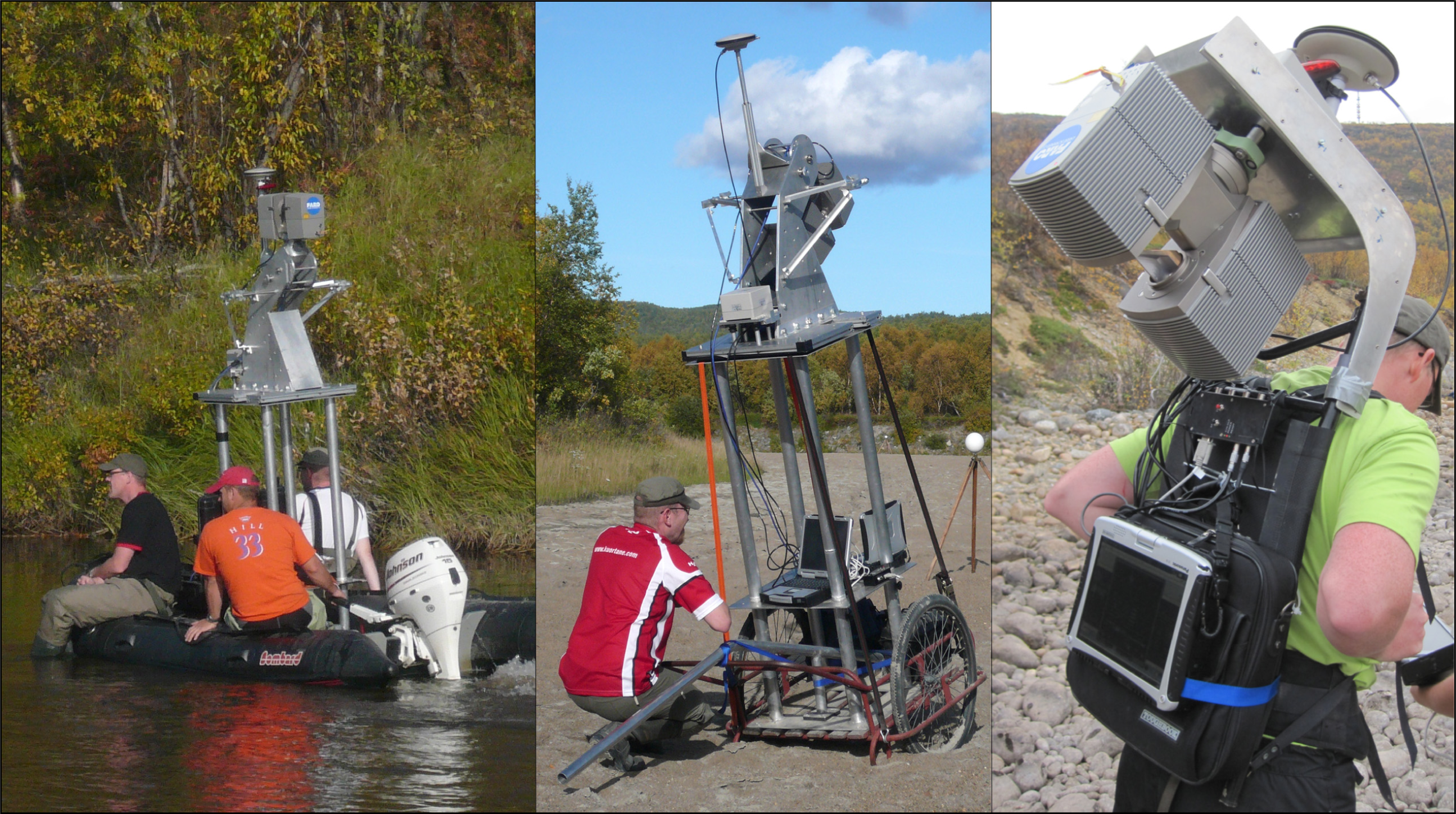
4.1.1. MLS Field Measurements (2010–2011)
4.1.2. MLS Data Processing
4.1.3. TLS Field Measurements (2010–2011)
4.2. UAV Photography
4.2.1. UAV Field Measurements (2010–2011)
4.2.2. UAV Image Processing (2010–2011)
4.3. UAV-Bathymery Modelling
4.3.1. Ground Data Measurements (2010–2011)
4.3.2. Building the Bathymetry DSM
5. Accuracy Assessment
6. Building the Seamless DTM
7. Change Detection
8. Discussion
9. Conclusions
Acknowledgments
Conflicts of Interest
References
- Veijalainen, N.; Lotsari, E.; Alho, P.; Vehviläinen, B.; Käyhkö, J. National scale assessment of climate change impacts on flooding in Finland. J. Hydrol 2010, 391, 333–350. [Google Scholar]
- Lotsari, E.; Wainwright, D.; Corner, G.; Alho, P.; Käyhkö, J. Surveyed and modelled one-year morphodynamics in the braided lower Tana River. Hydrol. Process. 2013. [Google Scholar] [CrossRef]
- Alho, P.; Hyyppä, H.; Hyyppä, J. Consequence of DTM precision for flood hazard mapping: A case study in SW Finland. Nord. J. Surv. Real Estate Res 2009, 6, 21–39. [Google Scholar]
- Hicks, D.M.; Shankar, U.; Duncan, M.J.; Rebuffé, M.; Aberle, J. Use of Remote-Sensing with Two-Dimensional Hydrodynamic Models to Assess Impacts of Hydro-Operations on a Large, Braided, Gravel-Bed River: Waitaki River, New Zealand. In Braided Rivers; Smith, G.H.S., Best, J.L., Bristow, C.S., Petts, G.E., Eds.; Blackwell Publishing Ltd: Malden, MA, USA, 2009; pp. 311–326. [Google Scholar]
- Vetter, M.; Hofle, B.; Mandlburger, G.; Rutzinger, M. Estimating changes of riverine landscapes and riverbeds by using airborne LiDAR data and river cross-sections. Z. Geomorphol. Suppl. Issues 2011, 55, 51–65. [Google Scholar]
- Williams, R.; Brasington, J.; Vericat, D.; Hicks, D. Hyperscale terrain modelling of braided rivers: Fusing mobile terrestrial laser scanning and optical bathymetric mapping. Earth Surf. Process. Landf. 2013. [Google Scholar] [CrossRef]
- Allouis, T.; Bailly, J.S.; Feurer, D. Assessing Water Surface Effects on LiDAR Bathymetry Measurements in Very Shallow Rivers: A Theoretical Study. Proceedings of the Second Space for Hydrology Workshop “Surface Water Storage and Runoff: Modeling, In-Situ Data and Remote Sensing”, Geneva, Switzerland, 12–14 November 2007.
- Feurer, D.; Bailly, J.S.; Puech, C.; Le Coarer, Y.; Viau, A.A. Very-high-resolution mapping of river-immersed topography by remote sensing. Prog. Phys. Geogr 2008, 32, 403–419. [Google Scholar]
- Lyzenga, D.R. Remote sensing of bottom reflectance and water attenuation parameters in shallow water using aircraft and Landsat data. Int. J. Remote Sens 1981, 2, 71–82. [Google Scholar]
- Best, J. The fluid dynamics of river dunes: A review and some future research directions. J. Geophys. Res. Earth Surf. 2005, 110. [Google Scholar] [CrossRef]
- Fuller, I.C.; Large, A.R.; Charlton, M.E.; Heritage, G.L.; Milan, D.J. Reach-scale sediment transfers: An evaluation of two morphological budgeting approaches. Earth Surf. Process. Landf 2003, 28, 889–903. [Google Scholar]
- Smith, M.J.; Chandler, J.; Rose, J. High spatial resolution data acquisition for the geosciences: Kite aerial photography. Earth Surf. Process. Landf 2009, 34, 155–161. [Google Scholar]
- Heritage, G.; Hetherington, D. Towards a protocol for laser scanning in fluvial geomorphology. Earth Surf. Process. Landf 2007, 32, 66–74. [Google Scholar]
- Cobby, D.M.; Mason, D.C.; Davenport, I.J. Image processing of airborne scanning laser altimetry data for improved river flood modelling. ISPRS J. Photogramm. Remote Sens 2001, 56, 121–138. [Google Scholar]
- Bates, P. Remote sensing and flood inundation modelling. Hydrol. Process 2004, 18, 2593–2597. [Google Scholar]
- Hyyppä, J.; Hyyppä, H.; Leckie, D.; Gougeon, F.; Yu, X.; Maltamo, M. Review of methods of small-footprint airborne laser scanning for extracting forest inventory data in boreal forests. Int. J. Remote Sens 2008, 29, 1339–1366. [Google Scholar]
- Mason, D.C.; Cobby, D.M.; Horritt, M.S.; Bates, P.D. Floodplain friction parameterization in two-dimensional river flood models using vegetation heights derived from airborne scanning laser altimetry. Hydrol. Process 2003, 17, 1711–1732. [Google Scholar]
- Kasvi, E.; Vaaja, M.; Alho, P.; Hyyppä, H.; Hyyppä, J.; Kaartinen, H.; Kukko, A. Morphological changes on meander point bars associated with flow structure at different discharges. Earth Surf. Process. Landf 2012, 38, 577–590. [Google Scholar]
- Wang, Y.; Liang, X.; Flener, C.; Kukko, A.; Kaartinen, H.; Kurkela, M.; Vaaja, M.; Hyyppä, H.; Alho, P. 3D modeling of coarse fluvial sediments based on mobile laser scanning data. Remote Sens 2013, 5, 4571–4592. [Google Scholar]
- El-Sheimy, N. An Overview of Mobile Mapping Systems. Proceedings of the From Pharaohs to Geoinformatics FIG Working Week 2005 and GSDI-8, Cairo, Egypt, 16–21 April 2005.
- Kukko, A.; Andrei, C.O.; Salminen, V.M.; Kaartinen, H.; Chen, Y.; Rönnholm, P.; Hyyppä, H.; Hyyppä, J.; Chen, R.; Haggrén, H.; et al. Road environment mapping system of the Finnish Geodetic Institute-FGI ROAMER. Int. Arch. Photogramm. Remote Sens. Spat. Inf. Sci 2007, 36, 241–247. [Google Scholar]
- Barber, D.; Mills, J.; Smith-Voysey, S. Geometric validation of a ground-based mobile laser scanning system. ISPRS J. Photogramm. Remote Sens 2008, 63, 128–141. [Google Scholar]
- Graham, L. Mobile mapping systems overview. Photogramm. Eng. Remote Sens 2010, 76, 222–228. [Google Scholar]
- Alho, P.; Kukko, A.; Hyyppä, H.; Kaartinen, H.; Hyyppä, J.; Jaakkola, A. Application of boat-based laser scanning for river survey. Earth Surf. Process. Landf 2009, 34, 1831–1838. [Google Scholar]
- Hohenthal, J.; Alho, P.; Hyyppä, J.; Hyyppä, H. Laser scanning applications in fluvial studies. Prog. Phys. Geogr 2011, 35, 782–809. [Google Scholar]
- Jaakkola, A.; Hyyppa, J.; Kukko, A.; Yu, X.; Kaartinen, H.; Lehtomaki, M.; Lin, Y. A low-cost multi-sensoral mobile mapping system and its feasibility for tree measurements. ISPRS J. Photogramm. Remote Sens 2010, 65, 514–522. [Google Scholar]
- Haarbrink, R.; Koers, E. Helicopter UAV for Photogrammetry and Rapid Response. Proceedings of the 2nd International Workshop “The Future of Remote Sensing”, Antwerp, Belgium, 17–18 October 2006; 36, p. 1.
- Sauerbier, M.; Eisenbeiss, H. UAVs for the documentation of archaeological excavations. Int. Arch. Photogramm. Remote Sens. Spat. Inf. Sci 2010, 38, 526–531. [Google Scholar]
- Remondino, F.; Barazzetti, L.; Nex, F.; Scaioni, M.; Sarazzi, D. UAV photogrammetry for mapping and 3d modeling—Current status and future perspectives. Int. Arch. Photogramm. Remote Sens. Spat. Inf. Sci 2011, 38, 1. [Google Scholar]
- Rosnell, T.; Honkavaara, E. Point cloud generation from aerial image data acquired by a quadrocopter type micro unmanned aerial vehicle and a digital still camera. Sensors 2012, 12, 453–480. [Google Scholar]
- Berni, J.; Zarco-Tejada, P.J.; Suárez, L.; Fereres, E. Thermal and narrowband multispectral remote sensing for vegetation monitoring from an unmanned aerial vehicle. IEEE Trans. Geosci. Remote Sens 2009, 47, 722–738. [Google Scholar]
- Koljonen, S.; Huusko, A.; Mäki-Petäys, A.; Louhi, P.; Muotka, T. Assessing habitat suitability for juvenile atlantic salmon in relation to in-stream restoration and discharge variability. Restor. Ecol 2012, 21, 344–352. [Google Scholar]
- Maxwell, S.L.; Smith, A.V. Generating river bottom profiles with a Dual-Frequency Identification Sonar (DIDSON). North Am. J. Fish. Manag 2007, 27, 1294–1309. [Google Scholar]
- Sirniö, V.P. Uoman Kartoitus-Teknologia. Maankäyttö 2004, 3, 26–27. [Google Scholar]
- Kaeser, A.J.; Litts, T.L.; Tracy, T.W. Using low-cost side-scan sonar for benthic mapping throughout the Lower Flint River, Georgia, USA. River Res. Appl 2013, 29, 634–644. [Google Scholar]
- Gao, J. Bathymetric mapping by means of remote sensing: Methods, accuracy and limitations. Prog. Phys. Geogr 2009, 33, 103–116. [Google Scholar]
- Hilldale, R.C.; Raff, D. Assessing the ability of airborne LiDAR to map river bathymetry. Earth Surf. Process. Landf 2008, 33, 773–783. [Google Scholar]
- Winterbottom, S.J.; Gilvear, D.J. Quantification of channel bed morphology in gravel-bed rivers using airborne multispectral imagery and aerial photography. Regul. Rivers-Res. Manag 1997, 13, 489–499. [Google Scholar]
- Westaway, R.; Lane, S.; Hicks, D. Remote survey of large-scale braided, gravel-bed rivers using digital photogrammetry and image analysis. Int. J. Remote Sens 2003, 24, 795–815. [Google Scholar]
- Gilvear, D.; Hunter, P.; Higgins, T. An experimental approach to the measurement of the effects of water depth and substrate on optical and near infra-red reflectance: A field-based assessment of the feasibility of mapping submerged instream habitat. Int. J. Remote Sens 2007, 28, 2241–2256. [Google Scholar]
- Flener, C.; Lotsari, E.; Alho, P.; Käyhkö, J. Comparison of empirical and theoretical remote sensing based bathymetry models in river environments. River Res. Appl 2012, 28, 118–133. [Google Scholar]
- Legleiter, C.; Roberts, D.; Marcus, W.; Fonstad, M. Passive optical remote sensing of river channel morphology and in-stream habitat: Physical basis and feasibility. Remote Sens. Environ 2004, 93, 493–510. [Google Scholar]
- Fonstad, M.; Marcus, W. Remote sensing of stream depths with hydraulically assisted bathymetry (HAB) models. Geomorphology 2005, 72, 320–339. [Google Scholar]
- Marcus, W.A.; Fonstad, M.A. Optical remote mapping of rivers at sub-meter resolutions and watershed extents. Earth Surf. Process. Landf 2008, 33, 4–24. [Google Scholar]
- Legleiter, C.; Roberts, D.; Lawrence, R. Spectrally based remote sensing of river bathymetry. Earth Surf. Process. Landf 2009, 34, 1039–1059. [Google Scholar]
- Flener, C. Estimating deep water radiance in shallow water: Adapting optical bathymetry modelling to shallow river environments. Boreal Environ. Res 2013, 18, 488–502. [Google Scholar]
- Legleiter, C.J.; Roberts, D.A. A forward image model for passive optical remote sensing of river bathymetry. Remote Sens. Environ 2009, 113, 1025–1045. [Google Scholar]
- Legleiter, C.J.; Overstreet, B.T. Mapping gravel bed river bathymetry from space. J. Geophys. Res. Earth Surf. 2012, 117. [Google Scholar] [CrossRef]
- Alho, P.; Mäkinen, J. Hydraulic parameter estimations of a 2D model validated with sedimentological findings in the point bar environment. Hydrol. Process 2010, 24, 2578–2593. [Google Scholar]
- Mansikkaniemi, H.; Mäki, O.P. Palaeochannels and recent changes in the Pulmankijoki valley, northern Lapland. Fennia 1990, 168, 137–152. [Google Scholar]
- Vaaja, M.; Kukko, A.; Kaartinen, H.; Kurkela, M.; Kasvi, E.; Flener, C.; Hyyppä, H.; Hyyppä, J.; Järvelä, J.; Alho, P. Data processing and quality evaluation of a boat-based mobile laser scanning system. Sensors 2013, 13, 12497–12515. [Google Scholar]
- Kukko, A.; Kaartinen, H.; Hyyppä, J.; Chen, Y. Multiplatform mobile laser scanning: Usability and performance. Sensors 2012, 12, 11712–11733. [Google Scholar]
- Axelsson, P. DEM generation from laser scanner data using adaptive TIN models. Int. Arch. Photogramm. Remote Sens. Spat. Inf. Sci 2000, 33, 111–118. [Google Scholar]
- Combrink, A. Introduction to Lidar-Based Aerial Surveys (Part 2). In PositionIT; EE Publishers: Muldersdrift, South Africa, 2011; pp. 20–24. [Google Scholar]
- Bilker, M.; Kaartinen, H. The Quality of Real-Time Kinematic (RTK) GPS Positioning; Reports of the Finnish Geodetic Institute: Masala, Finland, 2001. [Google Scholar]
- Schürch, P.; Densmore, A.L.; Rosser, N.J.; Lim, M.; McArdell, B.W. Detection of surface change in complex topography using terrestrial laser scanning: Application to the Illgraben debris-flow channel. Earth Surf. Process. Landf 2011, 36, 1847–1859. [Google Scholar]
- Milan, D.J.; Heritage, G.L.; Hetherington, D. Application of a 3D laser scanner in the assessment of erosion and deposition volumes and channel change in a proglacial river. Earth Surf. Process. Landf 2007, 32, 1657–1674. [Google Scholar]
- Bitenc, M.; Lindenbergh, R.; Khoshelham, K.; van Waarden, A.P. Evaluation of a LiDAR land-based mobile mapping system for monitoring sandy coasts. Remote Sens 2011, 3, 1472–1491. [Google Scholar]
- Marcus, W.; Legleiter, C.; Aspinall, R.; Boardman, J.; Crabtree, R. High spatial resolution hyperspectral mapping of in-stream habitats, depths, and woody debris in mountain streams. Geomorphology 2003, 55, 363–380. [Google Scholar]
- Carbonneau, P.E.; Lane, S.N.; Bergeron, N. Feature based image processing methods applied to bathymetric measurements from airborne remote sensing in fluvial environments. Earth Surf. Process. Landf 2006, 31, 1413–1423. [Google Scholar]
- Alho, P.; Vaaja, M.; Kukko, A.; Kasvi, E.; Kurkela, M.; Hyyppa, J.; Hyyppa, H.; Kaartinen, H.A. Mobile laser scanning in fluvial geomorphology: Mapping and change detection of point bars. Z. für Geomorphol 2011, 55, 31–50. [Google Scholar]
- Vaaja, M.; Hyyppä, J.; Kukko, A.; Kaartinen, H.; Hyyppä, H.; Alho, P. Mapping topography changes and elevation accuracies using a mobile laser scanner. Remote Sens 2011, 3, 587–600. [Google Scholar]
- Kasvi, E.; Alho, P.; Vaaja, M.; Hyyppä, H.; Hyyppä, J. Spatial and temporal distribution of fluvio-morphological processes on a meander point bar during a flood event. Hydrol. Res 2013, 44, 1022–1039. [Google Scholar]
- Entwistle, N.S.; Fuller, I.C. Terrestrial Laser Scanning to Derive the Surface Grain Size Facies Character of Gravel Bars. In Laser Scanning for the Environmental Sciences; Heritage, G.L.L.A., Ed.; Wiley-Blackwell: Oxford, UK, 2009; pp. 102–114. [Google Scholar]
- Lotsari, E.; Vaaja, M.; Flener, C.; Kaartinen, H.; Kukko, A.; Kasvi, E.; Hyyppä, H.; Hyyppä, J.; Alho, P. Detecting the morphological changes of banks and point bars in a meandering river using high-accuracy multi-temporal laser scanning and flow measurements. Water Resour. Res. 2013. submitted. [Google Scholar]


| Date | Scanner | Scanning Frequency (Hz) | Point Frequency (kHz) | Sensor Height (m) | Navigation System | Angular Resolution (°) | ||
|---|---|---|---|---|---|---|---|---|
| TLS | ||||||||
| 2010 | Leica HDS6100 | 25 | 213 | 2 | n/a | 0.036 | ||
| 2011 | Leica HDS6100 | 25 | 213 | 2 | n/a | 0.036 | ||
| BOMMS | ||||||||
| 2010 | 31.8. | Faro Photon 120 | 49 | 244 | 2.5 | NovAtel SPAN GPS-IMU | 0.072 | |
| 2011 | 8.9. | Faro Photon 120 | 49 | 244 | 2.5 | NovAtel SPAN GPS-IMU | 0.072 | |
| CartMMS | ||||||||
| 2010 | 31.8. | Faro Photon 120 | 49 | 244 | 2.3 | NovAtel SPAN GPS-IMU | 0.072 | |
| AkhkaMMS | ||||||||
| 2011 | 9.9. | Faro Photon 120 | 49 | 244 | 1.9 | NovAtel SPAN GPS-IMU | 0.072 | |
| Data Set | Reference Data | Vertical Adjustment | Average Magnitude | RMSE | min dz | max dz |
|---|---|---|---|---|---|---|
| Point bar data | ||||||
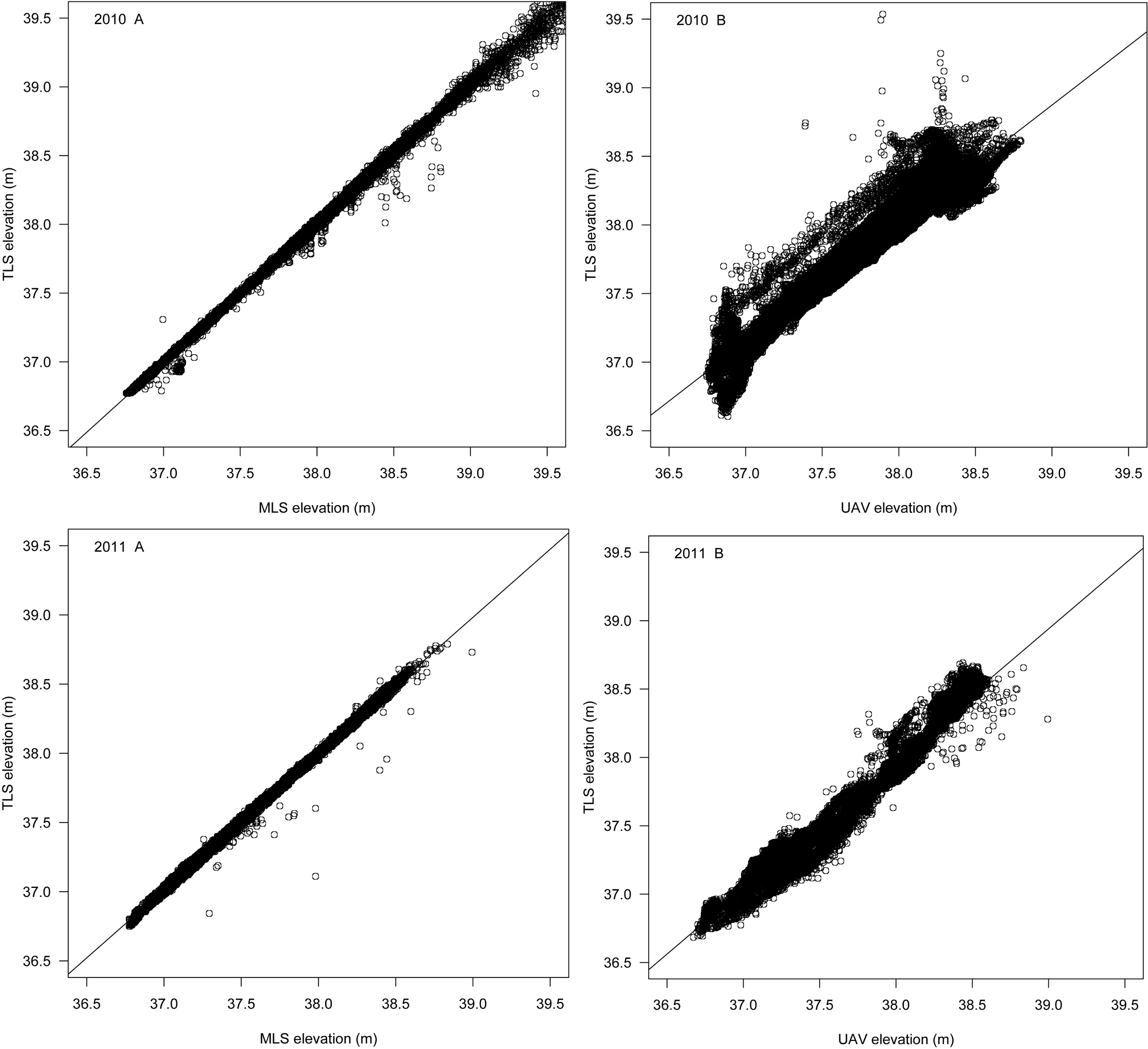
| MLS (BoMMS + CartMMS) 2010 | TLS points on pointbar | 0.01 | 0.0103 | 0.0151 | −1.1020 | +0.4920 |
| MLS (BOMMS + Akhka) 2011 | TLS points on pointbar | 0.01 | 0.0136 | 0.0182 | −0.8730 | +0.1210 |
| UAV-point-cloud 2010 | TLS points on pointbar | 0.03 | 0.0900 | 0.1520 | −0.3970 | +4.3640 |
| UAV-point cloud 2011 | TLS points on pointbar | 0.5 | 0.0705 | 0.088 | −0.7100 | +0.4990 |
| Riverbed data | ||||||
| UAV-bathymetry 2010 | Cross-validation | n/a | 0.097 | |||
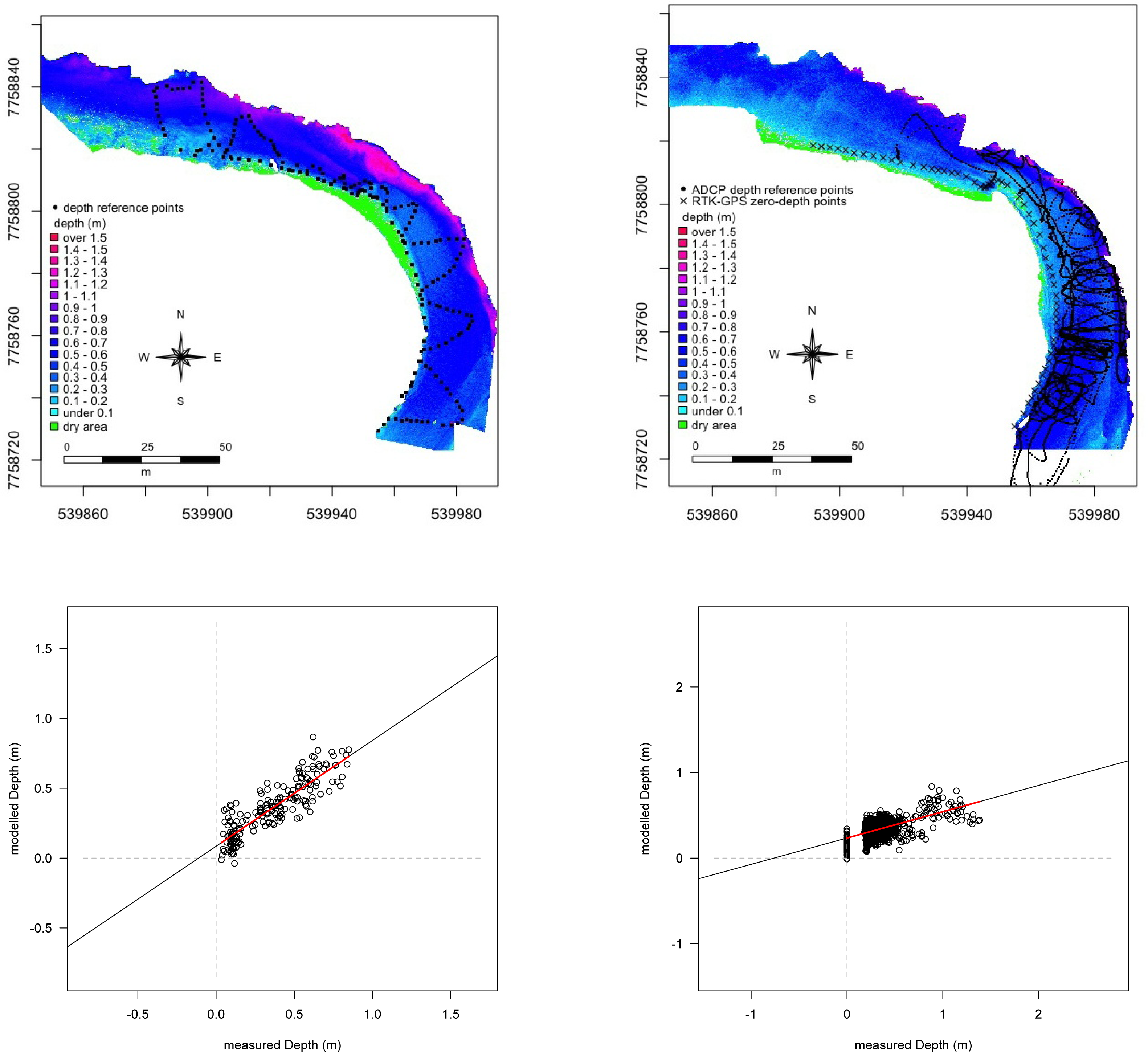
| UAV-bathymetry 2010 | RTK-GPS points | 0.12 | 0.1196 | 0.221 | −1.3503 | +1.3562 |
| UAV-bathymetry 2011 | Cross-validation | n/a | 0.078 | |||
| UAV-bathymetry 2011 | ADCP–RTK-GPS points | −0.50 | 0.117 | 0.163 | −1.015 | +0.460 |
© 2013 by the authors; licensee MDPI, Basel, Switzerland This article is an open access article distributed under the terms and conditions of the Creative Commons Attribution license ( http://creativecommons.org/licenses/by/3.0/).
Share and Cite
Flener, C.; Vaaja, M.; Jaakkola, A.; Krooks, A.; Kaartinen, H.; Kukko, A.; Kasvi, E.; Hyyppä, H.; Hyyppä, J.; Alho, P. Seamless Mapping of River Channels at High Resolution Using Mobile LiDAR and UAV-Photography. Remote Sens. 2013, 5, 6382-6407. https://doi.org/10.3390/rs5126382
Flener C, Vaaja M, Jaakkola A, Krooks A, Kaartinen H, Kukko A, Kasvi E, Hyyppä H, Hyyppä J, Alho P. Seamless Mapping of River Channels at High Resolution Using Mobile LiDAR and UAV-Photography. Remote Sensing. 2013; 5(12):6382-6407. https://doi.org/10.3390/rs5126382
Chicago/Turabian StyleFlener, Claude, Matti Vaaja, Anttoni Jaakkola, Anssi Krooks, Harri Kaartinen, Antero Kukko, Elina Kasvi, Hannu Hyyppä, Juha Hyyppä, and Petteri Alho. 2013. "Seamless Mapping of River Channels at High Resolution Using Mobile LiDAR and UAV-Photography" Remote Sensing 5, no. 12: 6382-6407. https://doi.org/10.3390/rs5126382