Article

Progress towards an Autonomous Field Deployable Diode-Laser-Based Differential Absorption Lidar (DIAL) for Profiling Water Vapor in the Lower Troposphere

1
Electrical and Computer Engineering, Montana State University, Bozeman, MT 59717, USA
2
National Center for Atmospheric Research, Boulder, CO 80307, USA
3
NASA Langley Research Center, Hampton, VA 23681, USA
4
Physics Department, Montana State University, Bozeman, MT 59717, USA
*
Author to whom correspondence should be addressed.
Remote Sens. 2013, 5(12), 6241-6259; https://doi.org/10.3390/rs5126241
Submission received: 31 August 2013 / Revised: 2 November 2013 / Accepted: 13 November 2013 / Published: 25 November 2013
(This article belongs to the Special Issue Optical Remote Sensing of the Atmosphere)

Abstract

:
A laser transmitter has been developed and incorporated into a micro-pulse differential absorption lidar (DIAL) for water vapor profiling in the lower troposphere as an important step towards long-term autonomous field operation. The laser transmitter utilizes two distributed Bragg reflector (DBR) diode lasers to injection seed a pulsed tapered semiconductor optical amplifier (TSOA), and is capable of producing up to 10 μJ of pulse energy with a 1 μs pulse duration and a 10 kHz pulse repetition frequency. The on-line wavelength of the laser transmitter can operate anywhere along the water vapor absorption feature centered at 828.187 nm (in vacuum) depending on the prevailing atmospheric conditions, while the off-line wavelength operates at 828.287 nm. This laser transmitter has been incorporated into a DIAL instrument utilizing a 35.6 cm Schmidt-Cassegrain telescope and fiber coupled avalanche photodiode (APD) operating in the photon counting mode. The performance of the DIAL instrument was demonstrated over a ten-day observation period. During this observation period, data from radiosondes were used to retrieve water vapor number density profiles for comparisons with the number density profiles retrieved from the DIAL data.

1. Introduction

The planetary boundary layer is the bottommost part of the troposphere and typically ranges from the Earth’s surface to several hundred meters, during stable nighttime conditions, to several kilometers, during the day, when solar induced convection causes shear and turbulence in the air parcel near the surface. Most of the convective processes that drive the Earth’s weather patterns initiate within the planetary boundary layer where most of the atmospheric water vapor and aerosols reside [1,2]. Understanding the state of the atmosphere requires knowledge of the spatial distribution of water vapor in the lower troposphere [3]. Research in the development of water vapor profiling tools to meet this needed measurement capability of water vapor distribution in the lower troposphere is ongoing [4,5].
Active optical remote sensing can be used for range resolved water vapor profile measurements in the lower troposphere. Two laser based active remote sensing techniques for water vapor profiling include Raman lidar [611] and differential absorption lidar (DIAL) [1220]. Raman lidar uses the characteristic frequency shift resulting from the inelastic Raman scattering to identify the molecular species of interest while DIAL utilizes the elastically scattered signals from two closely spaced laser transmitter wavelengths, the first associated with an absorption line for the molecule of interest, referred to as the on-line wavelength, and the second minimally affected by any molecular absorption, referred to as the off-line wavelength. The difference in the strength of the on-line and off-line return signals results from molecular absorption so that with knowledge of the absorption cross section, the ratio of scattered light collected by the DIAL receiver at the on-line and off-line wavelengths can be used to determine the molecular number density.
Modeling of low pulse energy, high pulse repetition rate DIAL instruments indicated that with the available avalanche photodiodes (APDs) operating in the photon counting Geiger mode, micro-pulse DIAL instruments are feasible with adequate spatial resolution and averaging times needed for monitoring water vapor in the lower troposphere [21,22]. The advantages of the diode-based micro-pulse DIAL include the ability to develop low-cost eye-safe instruments for autonomous network deployment, modularity, small footprint, and high wall plug efficiency. Recognizing the potential of the micro-pulse DIAL technique, Machol et al. [15] developed a diode-laser-based DIAL instrument based on distributed feedback (DFB) diode lasers and tapered semiconductor optical amplifiers (TSOAs) and demonstrated initial water vapor retrievals up to 2.5 km during nighttime operation. Building on the initial work of Machol et al., researchers at Montana State University have developed a micro-pulse DIAL based on two external cavity diode lasers (ECDL’s) and a single pulsed TSOA [1620]. This instrument has retrieved daytime water vapor profiles up to 4 km and nighttime water vapor profiles up to 6 km, providing the first demonstration of a diode-laser-based micro-pulse DIAL instrument capable of full-time water vapor and aerosol retrievals. However, the ECDL’s used in this instrument were prone to mode hopping inhibiting long term autonomous operation.
One major technological improvement over previously demonstrated instruments that is needed is the development of a stable laser transmitter, both spectrally and mechanically, capable of operating over long periods of time with minimal user interactions as an important step towards long term autonomous field deployment of micro-pulse DIAL instruments. A diode-laser-based micro-pulse DIAL is described in this manuscript that addresses improvements to the laser transmitter. The major improvement to the laser transmitter includes the elimination of the ECDL’s used by Nehrir et al. [1620], which would experience mode hops resulting from temperature changes in the local operating environment causing a loss in the frequency stabilization needed for long term DIAL operation. The ECDLs have been replaced by distributed Bragg reflector (DBR) diode lasers that are more stable against mechanical and thermal disturbances. Furthermore, many free space optical elements used in the laser transmitter have been replaced by fiber-coupled components as a further step in reducing the thermal and mechanical disturbances on optical alignment. To demonstrate the improvements resulting in the aforementioned hardware changes, the DIAL system was operated continuously during a ten-day observation period between 17 and 27 July 2013. The data products retrieved from the DIAL instrument during this observation period include the normalized relative backscatter and water vapor number density [19]. During this observational period, Vaisala RS92 radiosondes were launched providing temperature, pressure, and relative humidity profiles. Comparisons between the retrieved DIAL and radiosonde number density profiles were used to validate the DIAL measurements.
This paper is organized as follows: a description of the DIAL instrument is given in Section 2, a discussion of the data collected with the DIAL instrument is presented in Section 3, and concluding remarks are made in section 4.

2. Instrument

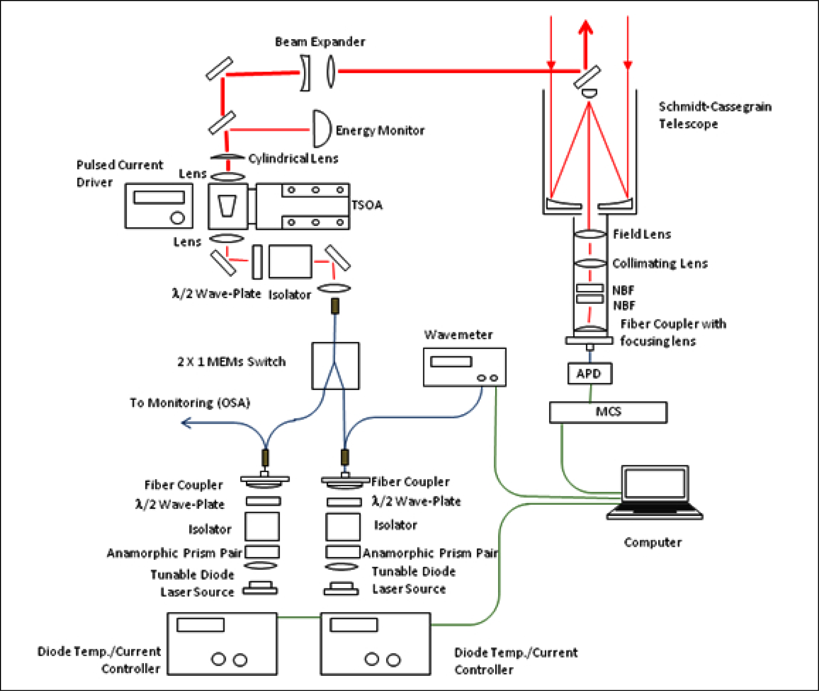
2.1. Laser Transmitter
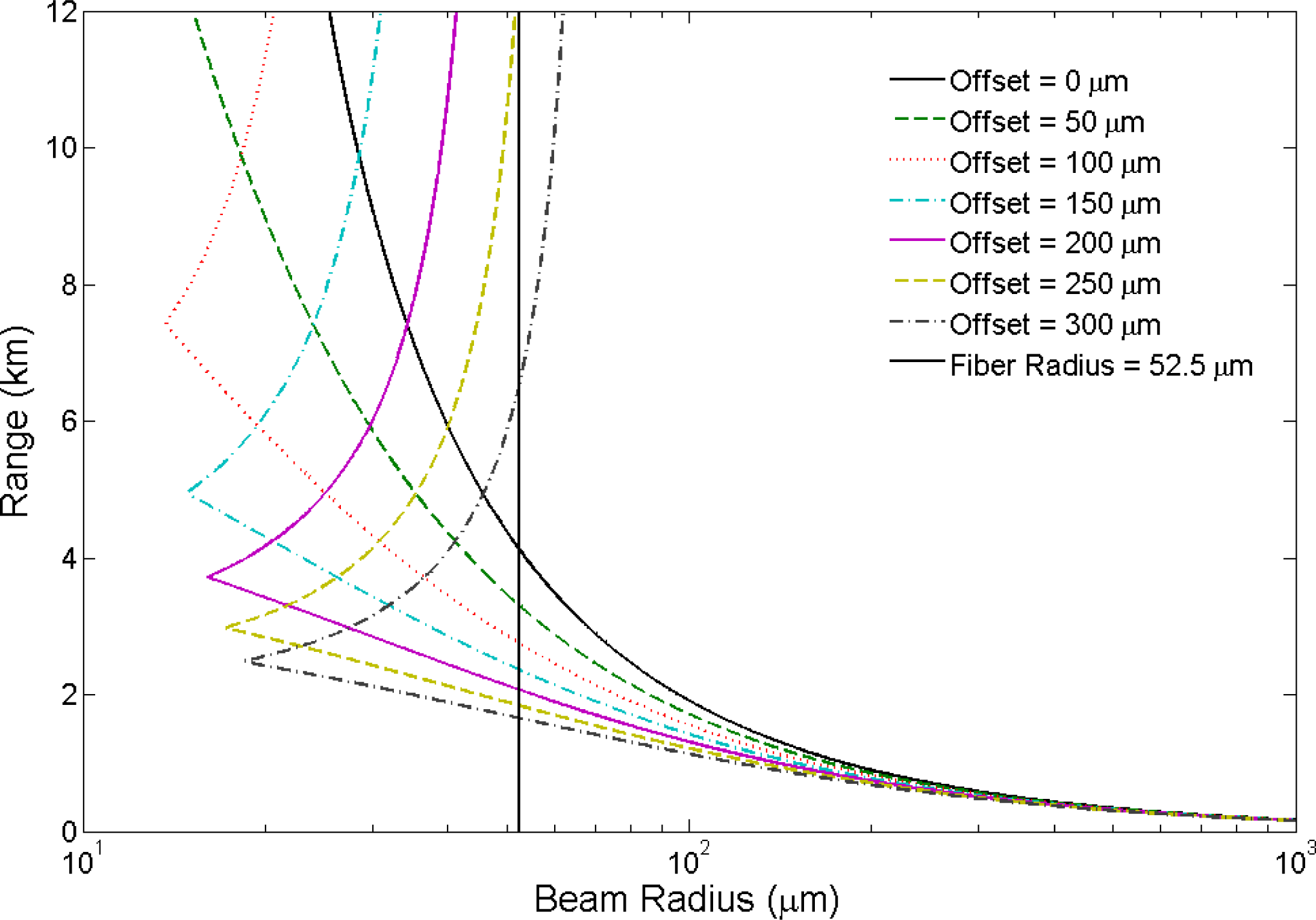
A schematic of the DIAL instrument is shown in Figure 1. The laser transmitter utilizes two DBR lasers mounted in a TO-8 package (manufactured by Photodigm, part number PH828DBR100T8) operating with a nominal wavelength of 828.2 nm. The laser linewidth was measured using a heterodyne technique based on mixing of two DBR laser to produce a beat note with a full width half maximum value of measured linewidth less than 1 MHz (0.023 pm). Each DBR laser can output up to 80 mW of continuous wave (cw) optical power and can be thermally tuned with a tuning response of 0.059 nm/C or tuned by adjusting the drive current with a tuning response of 0.0011 nm/mA. Each DBR laser is controlled using a commercial current and temperature controller (ILX Lightwave LDC3724C). The output from each DBR laser is collimated using an aspheric lens with a focal length of 4.0 mm and numerical aperture of 0.6. After the collimating lens, the cw light passes through a Faraday isolator (Thor Labs IO-3D-830-VLP) to prevent unwanted feedback and is then incident on a half-wave-plate to align the state of polarization to the polarization maintaining fibers. The cw light is then coupled into a single mode polarization maintaining fiber with angled physical contact (APC) connectors using an 11.0 mm focal length lens with a numerical aperture of 0.22. The polarization maintaining fiber delivers the light to a polarizartion maintaining 90/10 in-line fiber splitter (Newport F-PMC-850-10) with the 10% output port used for wavelength monitoring purposes while the 90% output port from each of the two laser assemblies is directed to a 2 × 1 fiber coupled micro-electro-mechanical systems (MEMS) switch (Aglitron LBPM-128238333).
The switch allows the injection seeding of the tapered semiconductor optical amplifier (TSOA) (Eagleyard EYP-TPA-830-01000-4006-CM-TO4) with either the on-line or off-line wavelength. Fiber coupled light from the switch is collimated using a lens with a focal length of 4.6 mm and a numerical aperture of 0.53 and next passes through a Faraday isolator to prevent unwanted feedback from the backward traveling amplified spontaneous emission from the TSOA entrance aperture to the seed lasers. After the Faraday isolator, the light is coupled into a 4.0 mm long ridge waveguide TSOA using a 4.5 mm focal length aspheric lens. The optical power of the seed laser for the on-line (off-line) wavelength right before the TSOA was 12.6 mW (13.9 mW). This seed power saturated the gain of the TSOA so that small changes in the input seed power did not appreciable affect the pulsed output energy of the TSOA. The output from the TSOA is collimated using a spherical lens, with a focal length of 4.5 mm, placed after the TSOA and a cylindrical lens with a focal length of 50 mm placed 79 mm after the spherical lens. These two lenses are needed to collimate the output of the TSOA, which exits from an output aperture of 3 μm × 190 μm. After the collimating lenses, approximately 2% of the light is directed to a low bandwidth photo detector used to monitor the output pulse energy while the remainder of the light is directed through a 5x beam expanded where the light is re-collimated. The collimated output beam has a measured M2 value of 2 in the vertical plane and 6 in the horizontal plane. The M2 value of 2 × 6 results in a full angle beam divergence of 14.6 μrad × 43.8 μrad for the 3.6 cm diameter collimated output beam. The field of view (FOV) of the receiver, which is discussed in detail in Section 2.2 below, is calculated to be 224 μrad.
The water vapor absorption line used has a center wavelength of 828.187 nm (in vacuum), a line-strength of 1.64 × 10⁻²³ cm−1/(molecule·cm−2), a full width at half maximum pressure broadened linewidth at sea level of γ0 = 0.1896 cm−1 (2.1 pm, 0.9 GHz), a linewidth temperature dependence of α = 0.74, and a ground state transitional energy of E” = 212.1564 cm−1 [1620,23]. The on-line DBR laser is stabilized with the aid of an optical wavemeter (EXFO-WA1500) using a feedback control loop in the data acquisition program. The wavemeter has a resolution of ±55 MHz (±0.125 pm) and a readout rate of 1 Hz. This resolution is larger than the laser linewidth of 1 MHz (0.23 pm) resulting in an uncertainty in the operating wavelength set by the resolution of the wavemeter. The on-line wavelength stabilization is achieved by reading the wavelength and comparing the DBR operating wavelength to a user defined set wavelength. If the operating wavelength varies from the set wavelength, the current to the DBR laser is adjusted to make small corrections to the DBR operating wavelength. The advantage for this method of frequency stabilization is that it allows operation of the on-line wavelength anywhere along the water vapor absorption feature, providing the user the ability to choose the absorption cross-section to match the prevalent atmospheric conditions. Ideally, the absorption cross section is set so that optical depth, τ, at the desired maximum altitude, rmax, is given by τ = 0 r max σ ( r , λ on ) N( r )d r 1 2 where σ(r, λ) is the absorption cross section and N(r) is the number density and the optical depth over a single range bin, Δτ, is given by Δτ = σ(r, λon)N(rr ≈ 0.02 − 0.1, where Δr is the range bin size [2426]. The off-line wavelength is set by adjusting the operating temperature and current at the beginning of the data collection period. This off-line laser is monitored using an optical spectrum analyzer with 0.06 nm (26 GHz) resolution. No active feedback control is provided to the off-line DBR laser.
Pulsed operation of the DIAL laser transmitter is achieved by pulsing the current to the TSOA. A commercial current driver capable of producing up to 15.7 A pulses up to 5 ms in pulse duration and up to 1 MHz pulse repetition frequency are used (Directed Energy, Inc, PCX-7420). The rise and fall time associated with the current pulse is 25 ns. For the DIAL operation, the pulse current driver was operated at 12.5 A with a 1 μs pulse duration and a 10 kHz pulse repetition frequency yielding a nominal pulse energy of 10.3 μJ. A summary of the laser transmitter parameters is given in Table 1.

2.2. DIAL Receiver

The receiver design described here closely follows the design previously described by Nehrir et al. [18,19]. Light scattered in the atmosphere is collected using a 35.56 cm diameter F/11 Schmidt-Cassegrain telescope. At the back end of the telescope, an adaptor was made to couple a lens tube assembly housing the receiver optics to the telescope. A field lens with a 2.54 cm diameter and a focal length of 7.5 cm was placed at the focal plane of the telescope. A collimating lens with a 2.54 cm diameter and focal length of 5 cm was placed 5 cm behind the field lens producing a nominally collimated beam with a beam diameter of 4.5 mm. The collimated light next passes through two narrowband interference filters. Each filter has a maximum transmission of T0 = 0.65, a center wavelength of λ0 = 828.206 nm, a half-width-half-maximum of Δλ = 125 pm. After the narrowband filters, a fiber coupler with a 4.6 mm clear aperture and a 1.1 cm focal length is used to couple the light into a step index optical fiber with a 105 μm diameter and a numerical aperture of 0.22, which acts as the receiver field stop. This is discussed in more detail below where a model of the optical receiver is developed.
Lidar instruments rely on the efficient delivery of the collected backscattered light to the detector. Micro-pulse lidar and micro-pulse DIAL instruments face the added challenge of minimizing the background light seen by the detector so that the small signal resulting from the low pulse energy can overcome the background signal. The DIAL receiver described in this paper utilizes an optical fiber to maintain a narrow field of view (FOV) to minimize the background light delivered to the detector. The design trade-off with maintaining the narrow FOV to try to minimize the background signal is the range at which the DIAL comes in to full overlap. The DIAL receiver design tries to strike a balance of maintaining the narrow FOV while achieving full overlap at an acceptable range.
A model of the DIAL receiver was developed to estimate the receiver performance in terms of overlap and FOV. The model is based on a ray-tracing analysis using the ABCD matrices [2729]. This analysis keeps track of the perpendicular distance, R, and slope, R′, of a ray relative to the optical axis using the vector:
R a = ( R R )
Each optical element is characterized by a 2 × 2 matrix. For the two optical elements needed for modeling the receiver, the 2 × 2 matrices are given by Equation (2a) for a lens, and Equation (2b) for free space propagation as:
M l = ( 1 0 1 / f 1 )
M f s = ( 1 d 0 1 )
where f is the focal length of the lens and d is the free space propagation distance. The optical system is characterized by the 2 × 2 matrix M = Mn Mn−1M2M1 where the subscript represents the order in which the optical element is encountered by the propagating ray. The output ray is then characterized by the vector Rb where Rb = MRa with the vector Ra characterizing the input ray.
The ray tracing analysis, outlined above, was used to model the optical receiver. This modeling assumes an outgoing beam radius of 2 cm with a full angle beam divergence of 25 μrad. The fiber, which acts as the field stop for the receiver, is located at the sum of the fiber coupling lens focal length plus an offset behind the fiber coupling lens. A plot of the beam radius at the fiber location is shown in Figure 2 as a function of range for various offsets. Overlap is achieved for the DIAL receiver when the beam radius is less than the fiber optic radius. For the optical receiver setup, light scattered from infinity will be imaged 1.1 cm behind the fiber coupling lens corresponding to a zero offset. However, as seen in Figure 2, overlap will not be achieved until a range of 4.1 km. By adjusting the offset, the range at which overlap is achieved can be reduced, however, if the offset is increased too far, the beam radius will become bigger than the fiber radius at larger ranges. The DIAL receiver offset was set at approximately 200 μm allowing full overlap to be achieved at 2.1 km while allowing the beam diameter to stay smaller than the fiber diameter up to 12 km.
For efficient coupling into the optical fiber, the incoming ray angles need to be less than the angle defined by the numerical aperture of the optical fiber. A plot of the maximum angle after the fiber lens as a function of range is shown in Figure 3. For the optical fiber used in the DIAL receiver, the maximum ray angle needs to be less than 0.22 radians, which, as seen from Figure 3, is achieved up to 12 km.
The field of view of the DIAL receiver is set by the optical fiber, which acts as the receiver field stop. The field of view is calculated by propagating rays from the optical fiber through the receiver optical elements using the ray propagation model described above. The full angle field of view is calculated to be 224 μrad. This narrow field of view is important as it sets the amount of background light that will be collected and delivered to the detector providing the main source of noise.
The receiver is monitored using a fiber coupled APD (Ecelitas SPCM-AQRH-13-FC) and a 20 MHz 4 channel multichannel scaler card (MCS) (Sigma Space AMCS-USB-4 Channel) data acquisition system. The laser transmitter generates pulses of 1 μs in duration corresponding to a range bin of 150 m; however, the MCS operates at 20 MHz, it collects a sample every 50 ns corresponding to a sampled range bin resolution of 7.5 m. Thus, the MCS collects 20 data points per 150 m pulse. During the post processing, 20 sampled range bins are summed to yield the 150 m range resolution of the DIAL instrument. A summary of the DIAL receiver specifications is given in Table 2.

2.1. Data Collection

The instrument is operated and data collected using the Labview programming environment. The on-line wavelength is actively locked by querying the optical wavemeter every 1 s and comparison of the operating wavelength of the DBR laser with a user defined operating wavelength allows adjustments to the on-line wavelength by varying the operating current of the on-line DBR laser. The MEMS switch is then set so that the on-line DBR laser seeds the TSOA and data collected over a user defined number of sampled range bins is averaged over 6 s using the MCS. The control program then reads the MCS and stores the data as a row in the on-line data matrix. Next, the MEMS switch is changed so that the off-line DBR laser is seeding the TSOA and the process is repeated with the data being stored in the off-line data matrix. The 6 s averaging time at each wavelength was chosen as a compromise between trying to capture rapidly changing atmospheric conditions and data transfer between the MCS and computer.
Data are processed in the matlab programming environment. First, the count rate for each range bin is estimated and the counting correction factor, given by Tc = 1/(1 − tdN) where td = 39.2 ns is the characteristic dead time associated with the APD, is applied for both the on-line and off-line return signals. Then, the last 50 sampled range bins are averaged for each return profile and this average value is used for background subtraction. The off-line wavelength returns are then used to generate the normalized relative backscatter profile using a 1 min averaging time while the on-line and off-line data are used to calculate the water vapor number density profile through application of the DIAL equation using a 20 min averaging time (10 min at each wavelength). The normalized relative backscatter retrieval uses a 150 m spatial averaging while the water vapor number density retrieval uses a 150 m spatial averaging below 3 km and a 300 m spatial averaging above 3 km. A flow chart summarizing the data processing is shown in Figure 4.

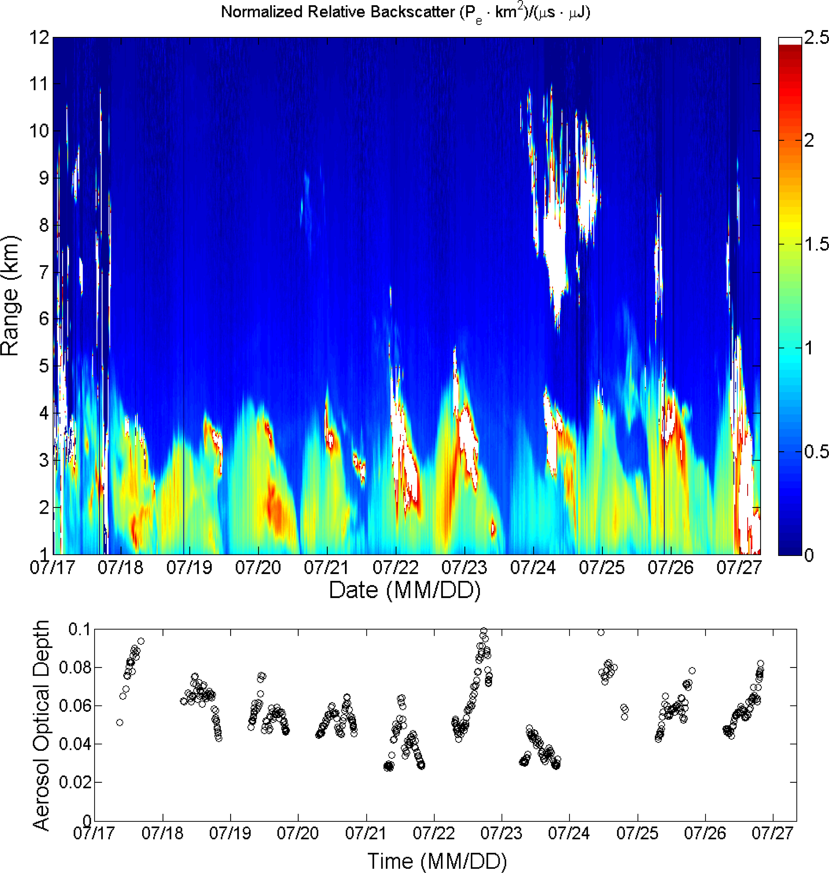
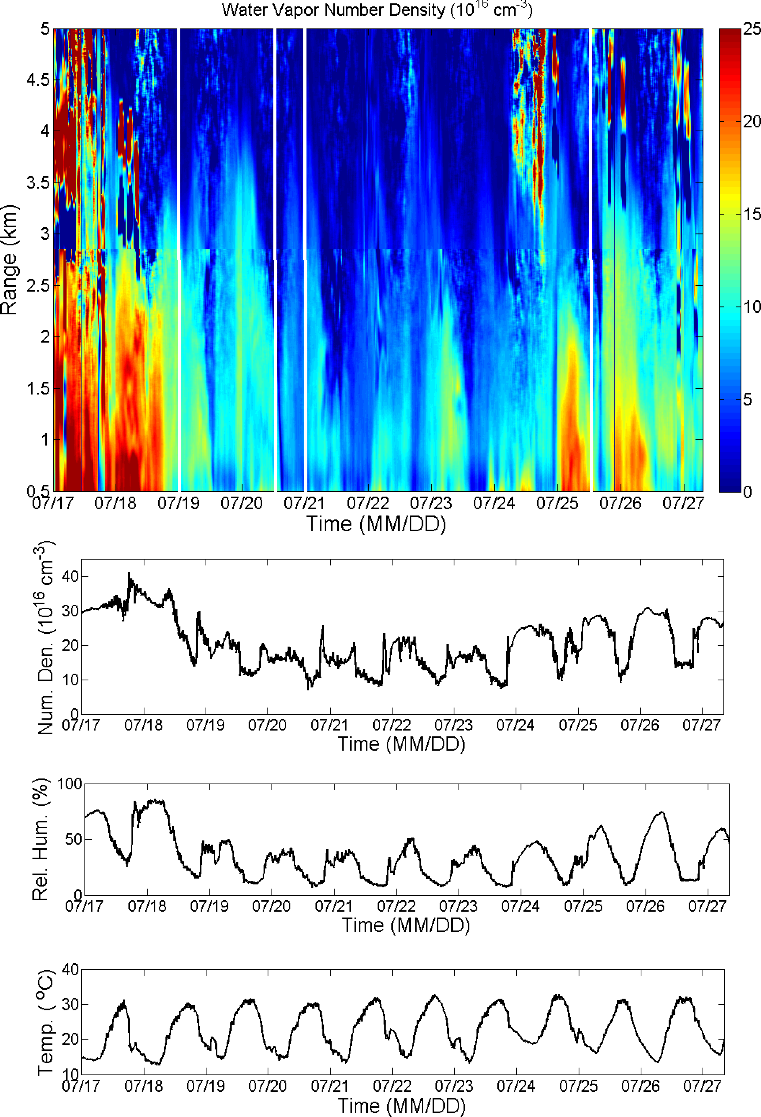
3. Observational Data

The DIAL instrument was operated over a ten-day period starting at 00:00 Mountain Daylight Time (MDT) 17 July 2013 and ending at 08:00 MDT 27 July 2013 at Montana State University. The DIAL operated in a laboratory environment with a major modification to the roof-port hatch allowing the installation of window for continuous operation regardless of meteorological conditions. The window has a 41 cm diameter and is not antireflection coated for the operating wavelength of the DIAL instrument coated. Measurement of the return signal with and without the window indicated that the window decreased the return signal by approximately 20% and will affect the signal to noise performance of the DIAL.
At the beginning of this observational period, storms occurred in western Montana as a frontal system moved through the area. By 19 July 2013, this frontal system moved out of the area and a high pressure system dominated resulted in clear skies. By 25 July 2013, another frontal system moved into the area for the remainder of the observation period.
The main data products for the micro-pulse DIAL include the normalized relative backscatter and the water vapor number density. The normalized relative backscatter provides qualitative information on the aerosol distribution and a plot of the normalized relative backscatter as a function of range and time is shown as the upper plot in Figure 5 for the ten-day observational period. Because the DIAL does not achieve full overlap until 2.1 km, an overlap correction factor needs to be applied for accurate retrieval of the normalized relative backscatter below 2.1 km. The correction factor can be determined experimentally by operating the instrument along a horizontal path or through modeling by utilizing the matrix derivation of the optical transfer function as described above. The aerosol optical depth measured by a co-located solar radiometer as part of the NASA AERONET program is shown in the bottom plot in Figure 5 for reference. The aerosol optical depth measured by AERONET ranges between 0.02 and 0.10 over the ten-day observational. The higher optical depths during this observational period most likely resulted from smoke from forest fires burning in the Western United States.
The water vapor number density as a function of time and range is shown as the upper plot in Figure 6 with the white vertical lines indicating radiosondes launches. Using a co-located ground-based weather station, the temperature, relative humidity, and water vapor number density at the surface is shown in the lower three plots of Figure 6. The frontal system present 17–18 July 2013 and the weaker frontal system 25–27 July 2013 resulted in higher water vapor number densities as seen in the upper plot of Figure 5, as compared to number densities seen 19–24 July 2013 when a high-pressure system dominated resulting in clear skies. During this observational period, the laser transmitter was operated at 828.2000 nm 17–18 July 2013 when relatively high water vapor number densities were present. Operating at 828.2000 nm changed the pressure broadened absorption cross section from its peak value of 5.51 × 10⁻²³ cm2 at line center to 1.10 × 10⁻²³ cm2. With the high pressure system resulting in clear skies 19–24 July 2013, the operating wavelength was changed to 828.1965 nm–828.1975 nm resulting in a pressure broadened absorption cross section of 1.81 × 10⁻²³ cm2–1.53 × 10⁻²³ cm2. With the weaker frontal system moving through 25–27 July 2013, the operating wavelength was increased to 828.1975 nm–828.1985 nm resulting in a pressure broadened absorption cross section of 1.53 × 10⁻²³ cm2–1.34 × 10⁻²³ cm2. The change in the on-line operating wavelength in response to the changing meteorological conditions was incorporated to try to maintain the optical depth between 1 and 2 at 5 km as discussed in Section 2.1 above.
During the observation period, Vaisala RS92 radiosondes were launched providing temperature, pressure and relative humidity profiles. A plot of the water vapor number density as a function of range for radiosondes launched 19 July 2013 at 00:16 MDT, 20 July 2013 at 21:55 MDT, 20 July 2013 at 12:45 MDT, and 25 July 2013 at 11:21 MDT are shown in the top-left, top-right, bottom-left, and bottom-right hand plots respectively in Figure 7. The red dashed line represents the number density retrieved from the temperature and relative humidity profiles measured by the radiosondes. The radiosonde profiles were filtered using a 20-point gliding filter corresponding to approximately a 60 m spatial average depending on the ascent rate of the radiosonde. The solid black line represents the DIAL retrieval at the time of the radiosonde launch. The error associated with the number density, Δn(r), is found as [30]:
Δ n ( r ) = 1 2 ( σ on ( r ) σ off ( r ) ) Δ r 1 m k { 1 N ( λ on , r ) + 1 N ( λ on , r + Δ r ) + 1 N ( λ off , r ) + 1 N ( λ off , r + Δ r ) } 1 2
where σon (r) (σon (r)) is the absorption on-line (off-line) absorption cross section at range r, m is the number of range bins averaged (m = 20 which corresponds to 150 m) and k is the number of samples in time (k = 100 which corresponds to one sample every six seconds averaged over 10 min), and N(λ,r) is the number of photons returned from range bin r at the wavelength λ. The grey shaded region represents the estimated error associated with the DIAL retrieval. The DIAL retrievals utilize a 20-minute averaging time and a 20-point gliding spatial filter corresponding to a 150 m spatial average. Good agreement between the radiosonde and DIAL profiles between 1.5 and 6 km for the two nighttime comparisons and between 1.5 and 4.5 km for the daytime comparisons is seen. Below 1.5 km, two factors can affect the DIAL retrieval including the range and wavelength dependent transmission of the narrow band optical filters [16,25] and the rapidly changing overlap function. For this micro-pulse DIAL, the pulse width is 1 μs resulting in a 150 m ambiguity in range to the scattering medium. As the overlap function can have large changes over this range, applying an accurate overlap correction becomes difficult, particularly at lower ranges where the overlap function changes most rapidly as a function of range.
During daytime operation of the DIAL, background solar radiation will affect the signal to noise ratio of the DIAL instrument. A plot of the normalized relative backscatter as a function of range and time is shown in the upper plot in Figure 7 for 20 July 2013. At 00:00 MDT, aerosols are present to approximately 4 km. As the day progresses, the aerosol layer falls to below 2 km by 15:00 MDT then begins to rise again to approximately 4 km by 24:00 MDT. This pattern was seen on the clear sky days between 19 July 2013 and 23 July 2013. The water vapor number density as a function of range and time is shown in the middle plot of Figure 8. The water vapor distribution follows a similar pattern as the aerosol distribution. The bottom plot in Figure 8 shows the background count rate as a function of time. This count rate was determined by considering the count rate in the last 50 range bins used for background subtraction. On clear sky days, the background count rate remains below 2 MHz, well below the maximum count rate of the APD. At this count rate, using the manufacturer supplied data to determine a dead time of td = 39.2 ns, the correction factor reaches a value of 1.09. Water vapor profiles can be obtained up to 6 km during nighttime operation and between 4 and 6 km during daytime operation depending on atmospheric conditions.
A plot of the normalized relative backscatter is shown as a function of range and time as the upper plot in Figure 9 for 24 July 2013. Clouds where present between 2 km and 4 km between 05:00 MDT and 07:00 MDT and between 6 km and 10 km between 00:00 MDT and 02:00 MDT, 05:00 MDT and 12:00 MDT, and 14:00 MDT and 22:00 MDT. A plot of the water vapor number density as a function of range and time is shown in middle plot in Figure 9, while the background count rate as a function of time is shown in the bottom plot in Figure 9. The background count rate reached a maximum value of 14 MHz resulting in a correction factor of 2.2. When the background count rate begins to get large, the dead time of the APD starts to play a significant role in limiting the detection of signal photons at both the on-line and off-line wavelengths. This becomes particularly important at higher ranges where, over a one second averaging time, the signal is on the order of tens of photons. These missed photons due to the detector dead time have an impact on the water vapor retrieval and result in limiting the water vapor retrieval to approximately 3.5 km.
The improvements to the laser transmitter described in this paper are aimed at moving the DIAL from a research tool to a field deployable instrument, capable of autonomous operation over extended periods of time. One of the major drawbacks to the prototype DIAL instrument was the tendency of the external cavity diode lasers to mode hop causing the seed lasers to lose their frequency stability requiring monitoring of the DIAL during data collection. The incorporation of the DFB lasers into the laser transmitter has eliminated mode hoping allow long term data collection as demonstrated by the data presented in this section. Furthermore, the DFB laser allows continuous tuning over approximately 1 nm, compared to the approximately 0.02 nm of mode hop free tuning associated with the external cavity diode lasers. This ability to continuously tune the seed laser along the absorption feature is useful in adjusting the absorption cross section for prevailing meteorological conditions, which will become important for deploying the DIAL instrument at various field sites.
The DIAL laser transmitter described in this paper is an important step in developing an autonomous, field deployable DIAL for water vapor profiling in the lower troposphere. To complete this development, improvements to the DIAL receiver need to be incorporated. The DIAL instrument described in this paper utilized a 35.6 cm diameter Schmidt-Cassegrain telescope that achieves full overlap at 2.1 km. A two channel receiver configuration that includes a near field channel and a far field channel is currently being incorporated into the DIAL receiver. The far field channel will have the same configuration described in this paper while the near field channel will utilize an APD with free space coupling to achieve full overlap at less than 0.5 km. This configuration will utilize a second channel on the multichannel scaler card currently used in the DIAL instrument. The other major improvement to the DIAL receiver will involve the incorporation an etalon into the receiver with a free spectral range equal to the frequency spacing between the on-line and off-line wavelengths to block solar background light that passes through the current narrowband filters. This etalon has the potential to improve daytime performance, particularly during cloudy conditions by limiting the background count rate.

4. Conclusions

Water vapor is the most dominant greenhouse gas in the atmosphere and plays an important role in many key atmospheric processes associated with both weather and climate. Water vapor is highly variable in space and time due to large-scale transport and biosphere-atmosphere interactions. Having long-term, high-resolution, vertical profiles of water vapor will help to better understand the water vapor structure and variability and its associated impact on weather and climate. The laser transmitter based on tunable DBR lasers and a TSOA described in this paper is an important step in the realization of an autonomous DIAL instrument for network deploy for water vapor studies in the lower troposphere. This laser transmitter produced a pulsed output with a nominal pulse energy of 10 μJ, a pulse duration of 1 μs, and a pulse repetition frequency of 10 kHz. This laser transmitter was incorporated into a micro-pulse DIAL instrument and operated continuously over a 10-day period demonstrating its ability for continuous and autonomous operation.

Acknowledgments

This work was supported under the kind auspices of the National Science Foundation grant number 1206166.

Conflicts of Interest

The authors declare no conflict of interest.

References

  1. Emanuel, K.; Raymond, D.; Betts, A.; Bosart, L.; Bretherton, C.; Droegemeir, K.; Farrell, B.; Fritsch, J.M.; Houze, R.; Lemone, M.A.; et al. Report of the First Prospectus Development Team of the U.S. Weather Research Program to NOAA and the NSF. Bull. Am. Meteor. Soc 1995, 76, 1194–1208. [Google Scholar]
  2. Dabberdt, W.F.; Schlatter, T.W. Research opportunities from emerging atmospheric observing and modeling capabilities. Bull. Am. Meteor. Soc 1996, 77, 305–323. [Google Scholar]
  3. Weckwerth, T.M.; Wulfmeyer, V.; Wakimoto, R.M.; Hardesty, R.M.; Wilson, J.W.; Banta, R.M. NCAR-NOAA lower tropospheric water vapor workshop. Bull. Am. Meteor. Soc 1999, 80, 2339–2357. [Google Scholar]
  4. Carbone, R.E.; Block, J.; Boselly, S.E.; Carmichael, G.R.; Carr, F.H.; Chandrasekar, V.; Gruntfest, E.; Hoff, R.H.; Krajewski, W.F.; LeMone, M.A.; et al. Observing Weather and Climate from the Ground Up: A Nationwide Network of Networks; National Academy Press: Washington, DC, USA, 2009. [Google Scholar]
  5. Hooff, R.M.; Hardesty, R.M.; Carr, F.; Weckwerth, T.; Koch, S.; Benedetti, A.; Crewell, S.; Cimini, N.; Turner, D.; Feltz, W.; et al. Thermodynamic Profiling Technologies Workshop, Report to the National Science Foundation and the National Weather Service; Hardesty, R.M., Hoff, R.M., Eds.; National Center for Atmospheric Research: Boulder, CO, USA, 2011. [Google Scholar]
  6. Whiteman, D.N.; Melfi, S.H.; Ferrare, R.A. Raman lidar system for the measurement of water vapor and aerosols in the Earth’s atmosphere. Appl. Opt 1992, 31, 3068–3082. [Google Scholar]
  7. Whiteman, D.N.; Rush, K; Rabenhorst, S.; Welch, W; Cadirola, M; McIntire, G; Russo, F.; Adam, M; Venable, D.; Connell, R.; et al. Airborne and ground-based measurements using a high-performance raman lidar. J. Atmos. Oceanic Technol 2010, 27, 1781–1801. [Google Scholar]
  8. Wandinger, U. Raman Lidar. In Lidar: Range-Resolved Optical Remote Sensing of the Atmosphere; Weitkamp, C., Ed.; Springer: Berlin, Germany, 2005; pp. 241–271. [Google Scholar]
  9. Whiteman, D. Examination of the traditional Raman lidar technique. II: Evaluating the ratios for water vapor and aerosols. Appl. Opt 2003, 42, 2593–2608. [Google Scholar]
  10. Mattis, I.; Jaenisch, V. Automated Lidar Data Analyzer (ALDA) for RAMSES—The Autonomously Operating German Meteorological Service Raman Lidar for Atmospheric Moisture Sensing. Proceedings of 23rd International Laser Radar Conference, Nara, Japan, 24–28 July 2006; pp. 215–218.
  11. Leblanc, T.; McDermid, I.S.; Aspey, R.A. First-year operation of a new water vapor Raman lidar at the JPL Table Mountain Facility, California. J. Atmos. Ocean. Technol 2008, 25, 1454–1462. [Google Scholar]
  12. Higdon, N.S.; Browell, E.V.; Ponsardin, P.; Grossmann, B.E.; Butler, C.F.; Chyba, T.H.; Mayo, M.N.; Allen, R.J.; Heuser, A.W.; Grant, W.B.; et al. Airborne differential absorption lidar system for measurements of atmospheric water vapor and aerosols. Appl. Opt 1994, 33, 6422–6438. [Google Scholar]
  13. Didier, B.; Quaglia, P.; Flamant, C.; Meissonnier, M.; Pelon, J. Airborne Lidar LEANDRE II for Water-Vapor Profiling in the Troposphere. I. System description. Appl. Opt 2001, 40, 3450–3461. [Google Scholar]
  14. Wirth, M.; Fix, A.; Mahnke, P.; Schwarzer, H.; Schrandt, F.; Ehret, G. The airborne multi-wavelength water vapor differential absorption lidar WALES: System design and performance. Appl. Phys. B 2009, 96, 201–213. [Google Scholar]
  15. Machol, J.L.; Ayers, T.; Schwenz, K.T.; Koenig, K.W.; Hardesty, R.M.; Senff, C.J.; Krainak, M.A.; Abshire, J.B.; Bravo, H.E.; Sandberg, S.P. Preliminary measurements with an automated compact differential absorption lidar for profiling water vapor. Appl. Opt 2004, 43, 3110–3121. [Google Scholar]
  16. Nehrir, A.R.; Repasky, K.S.; Carlsten, J.L.; Obland, M.D.; Shaw, J.A. Water vapor profiling using a widely tunable, amplified diode Laser based differential absorption lidar (DIAL). J. Atmos. Ocean. Technol 2009, 26, 733–745. [Google Scholar]
  17. Nehrir, A.R. Water Vapor Profiling using a Compact Widely Tunable Diode Laser Differential Absorption Lidar (DIAL). Montana State University, Bozeman, MT, USA, November 2008. [Google Scholar]
  18. Nehrir, A.R.; Repasky, K.S.; Carlsten, J.L. Eye-safe diode-laser-based micropulse differential absorption lidar (DIAL) for water vapor profiling in the lower troposphere. J. Atmos. Ocean. Technol 2011, 28, 131–147. [Google Scholar]
  19. Nehrir, A.R. Development of an eye-safe diode-laser-based micro-pulse differential absorption lidar (MP_DIAL) for atmospheric water vapor and aerosol studies, Montana State University, Bozeman, MT, USA, July 2011.
  20. Nehrir, A.R.; Repasky, K.S.; Carlsten, J.L. Micropulse water-vapor differential absorption lidar: transmitter design and performance. Opt. Express 2012, 20, 25137–25151. [Google Scholar]
  21. Reagan, J.A.; Cooley, T.W.; Shaw, J.A. Prospects for an Economical, Eye Safe Water Vapor Lidar. Proceedings of the IEEE International Geoscience and Remote Sensing Symposium, Tokyo, Japan, 18–21 August, 1993; pp. 872–874.
  22. Reagan, J.A.; Liu, H; McCalmont, J.F. Laser Diode Based New Generation Lidars. Proceedings of the IEEE International Geoscience and Remote Sensing Symposium, Lincoln, NE, USA, 27–31 May 1996; pp. 1535–1537.
  23. Rothman, L.S.; Gordon, I.E.; Barbe, A.; Benner, D.C.; Bernath, P.F.; Birk, M.; Boudon, V.; Brown, L.R.; Campargue, A.; Champion, J.P.; et al. The HITRAN 2008 molecular spectroscopic database. J. Quant. Spectrosc. Radiat. Transf 2009, 110, 533–572. [Google Scholar]
  24. Remsberg, E.E.; Gordley, L.L. Analysis of differential absorption lidar from the Space Shuttle. Appl. Opt 1978, 17, 624–630. [Google Scholar]
  25. Wulfmeyer, V.; Bosenberg, J. Ground-based differential absorption lidar for water vapor profiling: Assesment of accuracy, resolution, and meteorological applications. Appl. Opt 1998, 37, 3825–3844. [Google Scholar]
  26. Bosenberg, J. Ground-based differential absorption lidar for water-vapor profiling: Methodology. Appl. Opt 1998, 37, 3845–3860. [Google Scholar]
  27. Siegman, A.A. Lasers; University Science Books: Sausalito, CA, USA, 1986. [Google Scholar]
  28. Yariv, A. Quantum Electronics, 2nd ed.; John Wiley and Sons: New York, NY, USA, 1975. [Google Scholar]
  29. Saleh, B.E.A.; Teich, M.C. Fundamentals of Photonics, 2nd ed; John Wiley and Sons: Hoboken, NJ, USA, 2007. [Google Scholar]
  30. Wulfmeyer, V.; Walther, C. Future performance of ground-based and airborne water-vapor differential absorption lidar. I. overview and theory. Appl. Opt 2001, 40, 5304–5320. [Google Scholar]
Figure 1. Schematic of the diode laser based DIAL instrument. The Laser transmitter is based on two DBR lasers used to injection seed a TSOA in a MOPA configuration.
Remotesensing 05 06241f1
Figure 2. The beam radius at the optical fiber as a function of range and offset. The fiber radius is 52.5 μm as is shown as the vertical solid black line. Overlap occurs when the beam radius is less than the fiber radius.
Remotesensing 05 06241f2
Figure 3. The maximum ray angle at the optical fiber as a function of range. The fiber numerical aperture requires angles less than 0.22 radians for efficient coupling. The vertical red dashed line indicated the maximum ray angle accepted by the optical fiber.
Remotesensing 05 06241f3
Figure 4. A flow chart summarizing of the data processing.
Remotesensing 05 06241f4
Figure 5. A plot of the normalized relative backscatter as a function of range and time is shown in the upper plot. The corresponding aerosol optical depth at 830 nm measured with a co-located solar radiometer as part of the NASA AERONET program is shown in the bottom plot.
Remotesensing 05 06241f5
Figure 6. The water vapor number density as a function of range and time is shown in the top plot while the number density, relative humidity, and temperature measures at the surface are shown in the bottom three plots. The solid white vertical lines in the top plot indicate radiosonde launches.
Remotesensing 05 06241f6
Figure 7. Plots of the water vapor number density as a function of range for data collect 19 July 2013 at 00:16, 20 July 2013 at 21:55, 20 July 2013 at 12:45, and 25 July 2013 at 11:21, are shown in the top left, top right, bottom left, and bottom right plots, respectively. The dashed red line represents retrieved number density profiles based on the temperature and relative humidity measured by the radiosonde while the solid black line represents the water vapor number density retrieved from the DIAL at the time of the radiosonde launch. The upper left-hand, upper right-hand, lower left-hand, and lower right-hand plots.
Remotesensing 05 06241f7
Figure 8. The upper plot shows the normalized relative backscatter as a function of time and range for 20 July 2013, while the middle figure shows the corresponding water vapor number density as a function of range and time. The bottom figure shows the background count rate as a function of time measured using the last fifty ranges bins. For clear sky operations, the maximum background count rate is less than 2 MHz and water vapor retrievals during daytime operations can be achieved between 4 and 6 km depending on atmospheric conditions.
Remotesensing 05 06241f8
Figure 9. The upper plot shows the normalized relative backscatter as a function of time and range for 24 July 2013, while the middle figure shows the corresponding water vapor number density as a function of range and time. The bottom figure shows the background count rate as a function of time measured using the last fifty ranges bins. Operations during cloudy conditions result in maximum background count rates exceeding 14 MHz and water vapor retrievals during daytime operations can be achieved between 3 and 3.5 km depending on atmospheric conditions.
Remotesensing 05 06241f9
Table 1. A summary of the laser transmitter parameters. The short-term linewidth resulted from the heterodyne measurement, while the long-term bandwidth results from the resolution of the wavemeter used to lock the on-line seed laser.
ParameterMeasured
Laser Seeder2 DBR diode lasers
AmplifierSingle Stage TSOA
828.187 nm (on-line)
Transmitter Wavelengths828.1965–828.2000 nm (side-line)
828.287 nm (off-line)
Pulse Duration1 μs
Pulse Repetition Rate10 kHz
Pulse Energy10 μJ
Short Term Linewidth<1 MHz (0.023 pm)
Long Term Bandwidth±55 MHz ± (0.125 pm)
Beam Diameter3.8 cm
Switching Time6 s
Averaging Time20 min
Table 2. A summary of the differential absorption lidar (DIAL) receiver parameters.
ParameterMeasured
TelescopeSchmidt-Cassegrain
Primary Mirror Diameter35.56 cm
Full Angle Field of View224 μrad
DetectorSi Photon Counting APD
APD Quantum Efficiency45%
Optical Filter Bandwidth250 pm
Range Resolution150 m

