A Water Index for SPOT5 HRG Satellite Imagery, New South Wales, Australia, Determined by Linear Discriminant Analysis

Abstract
:1. Introduction
1.1. Water Indices
2. Method
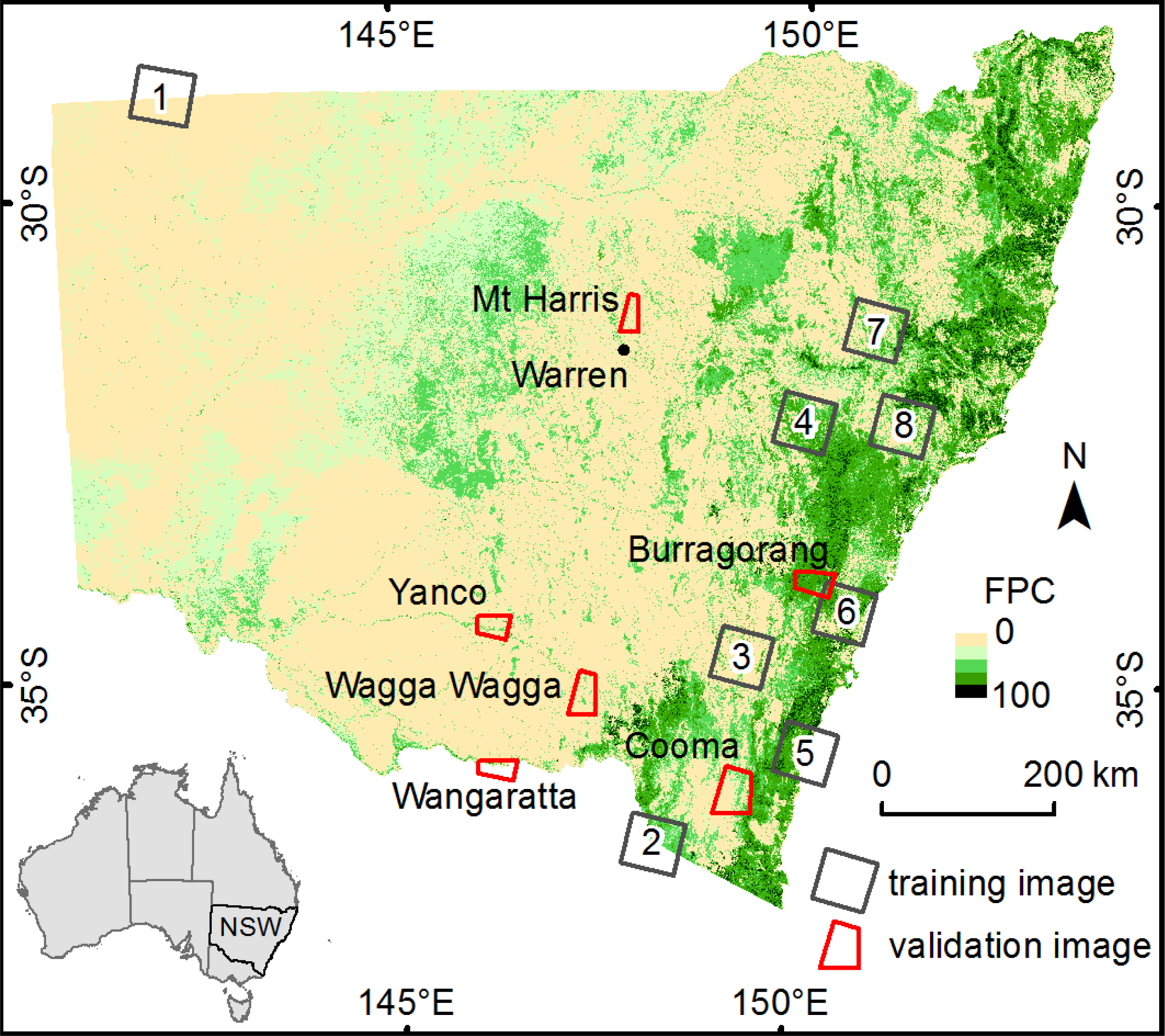
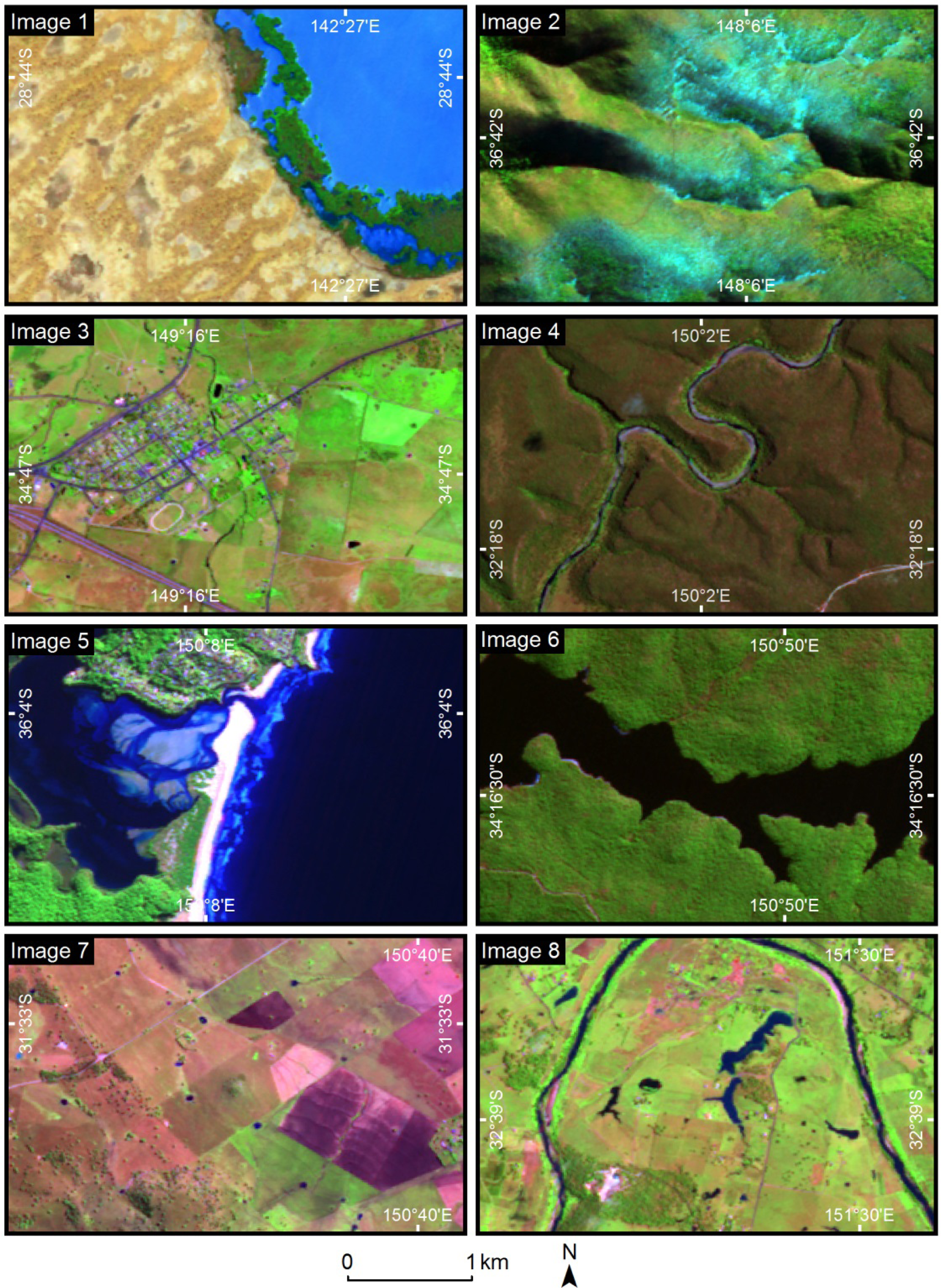
2.1. Data
2.2. Pre-Processing
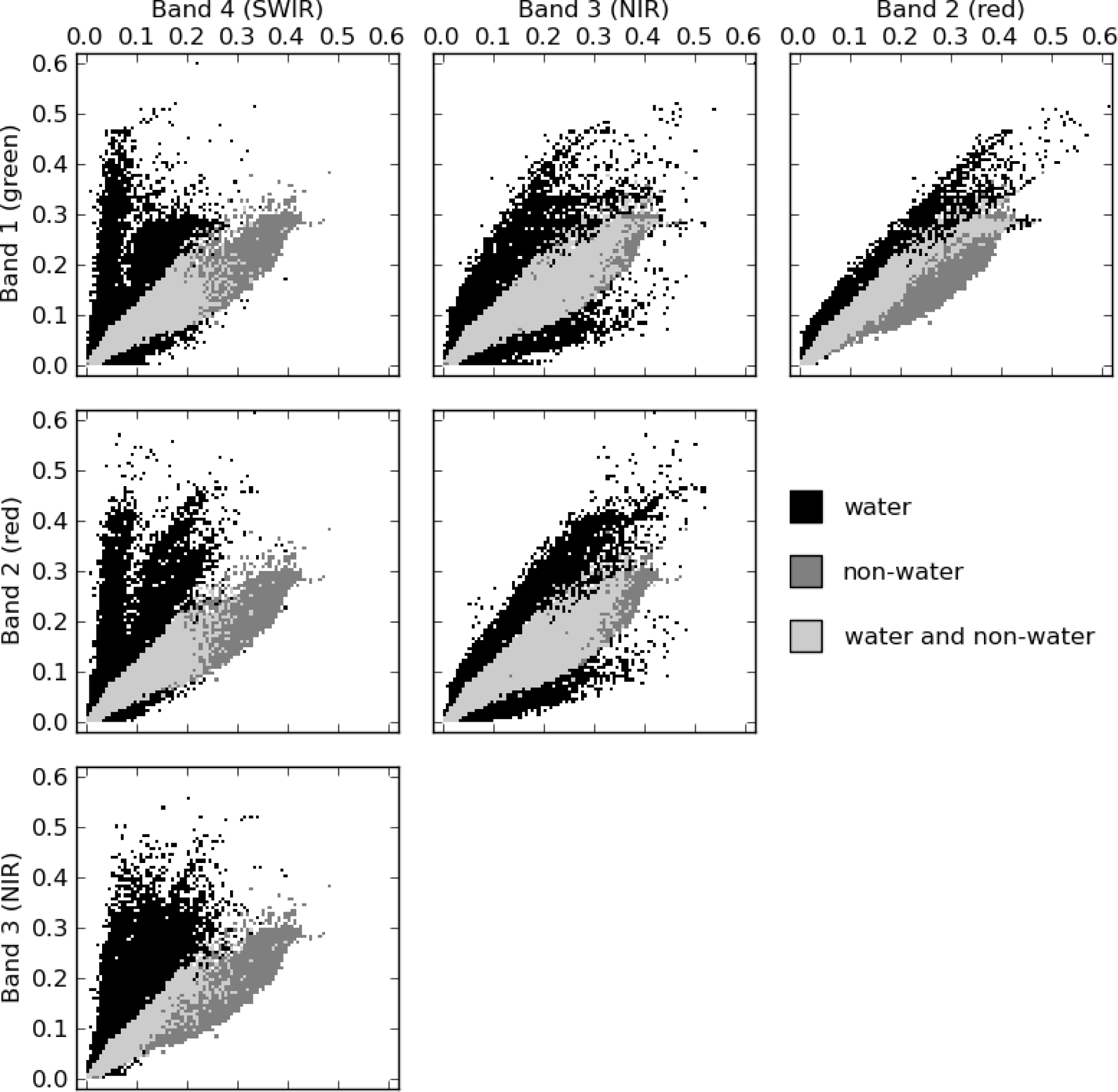
2.3. Training Data
2.4. Linear Discriminant Analysis Classification
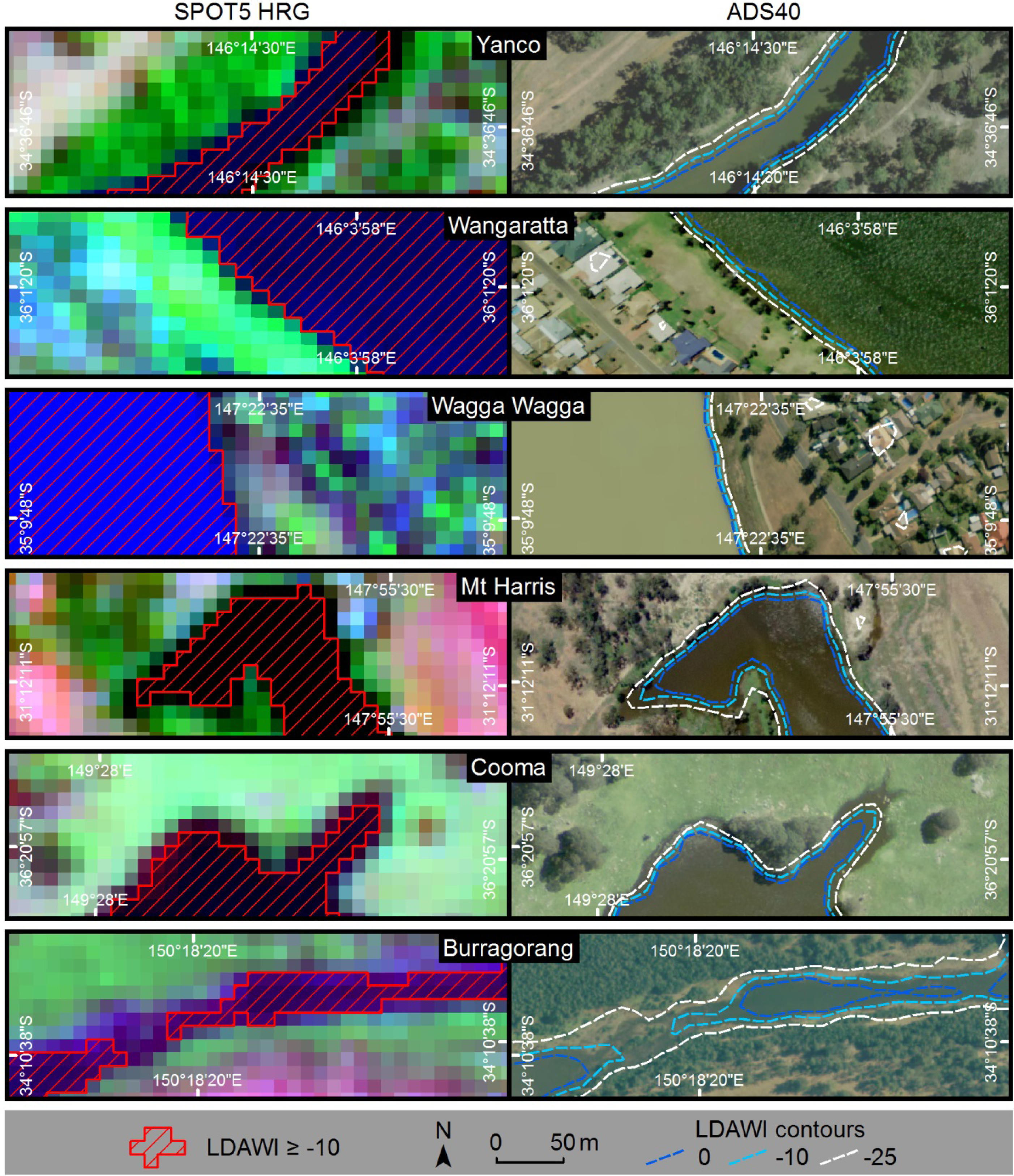
2.5. Validation Data
3. Results and Accuracy Assessment
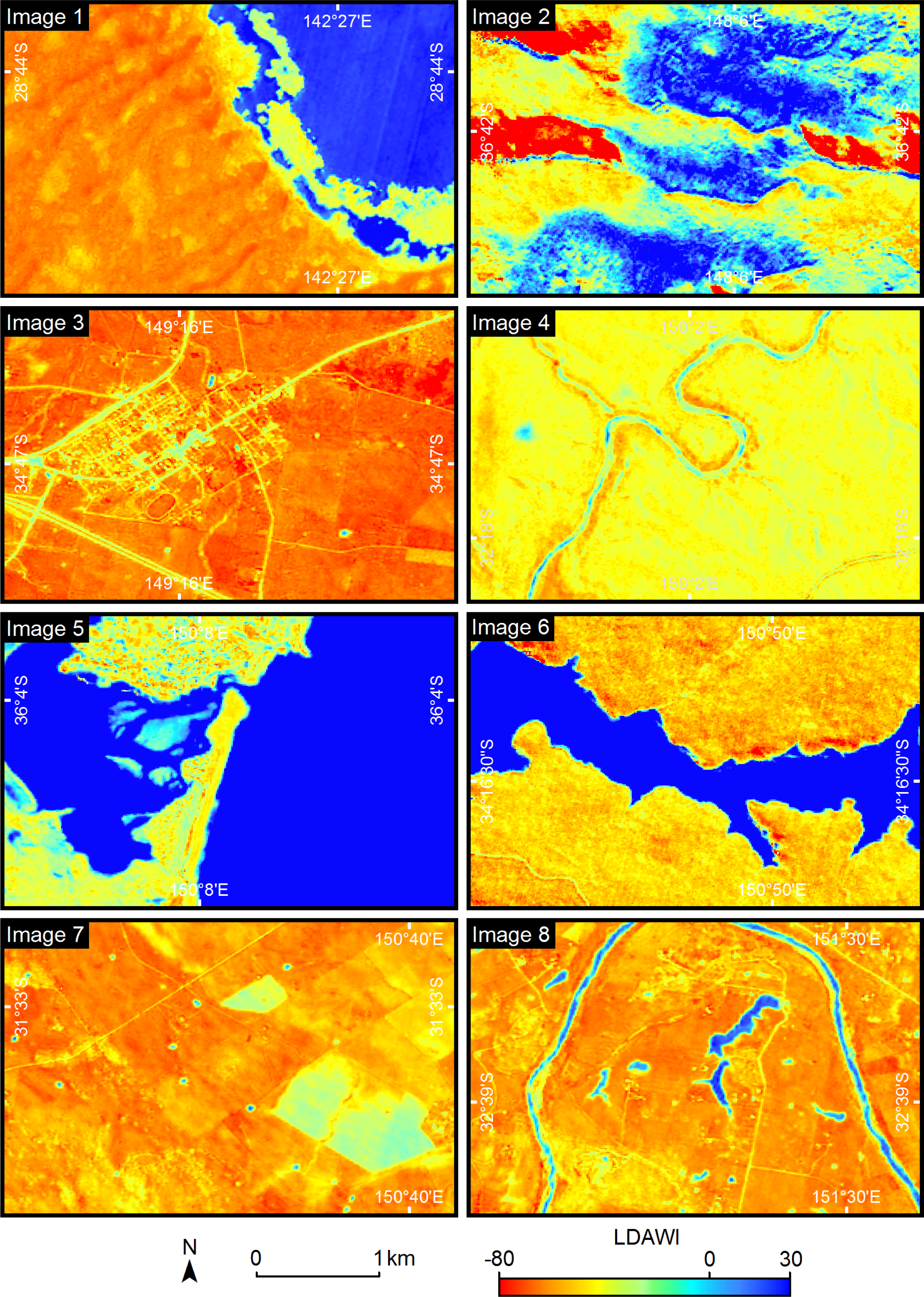
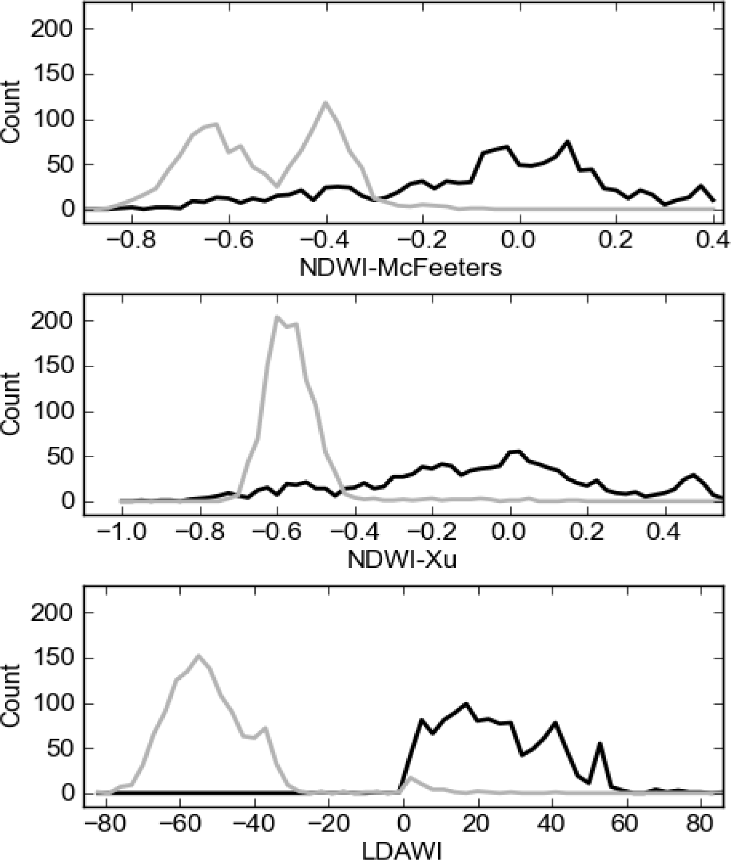
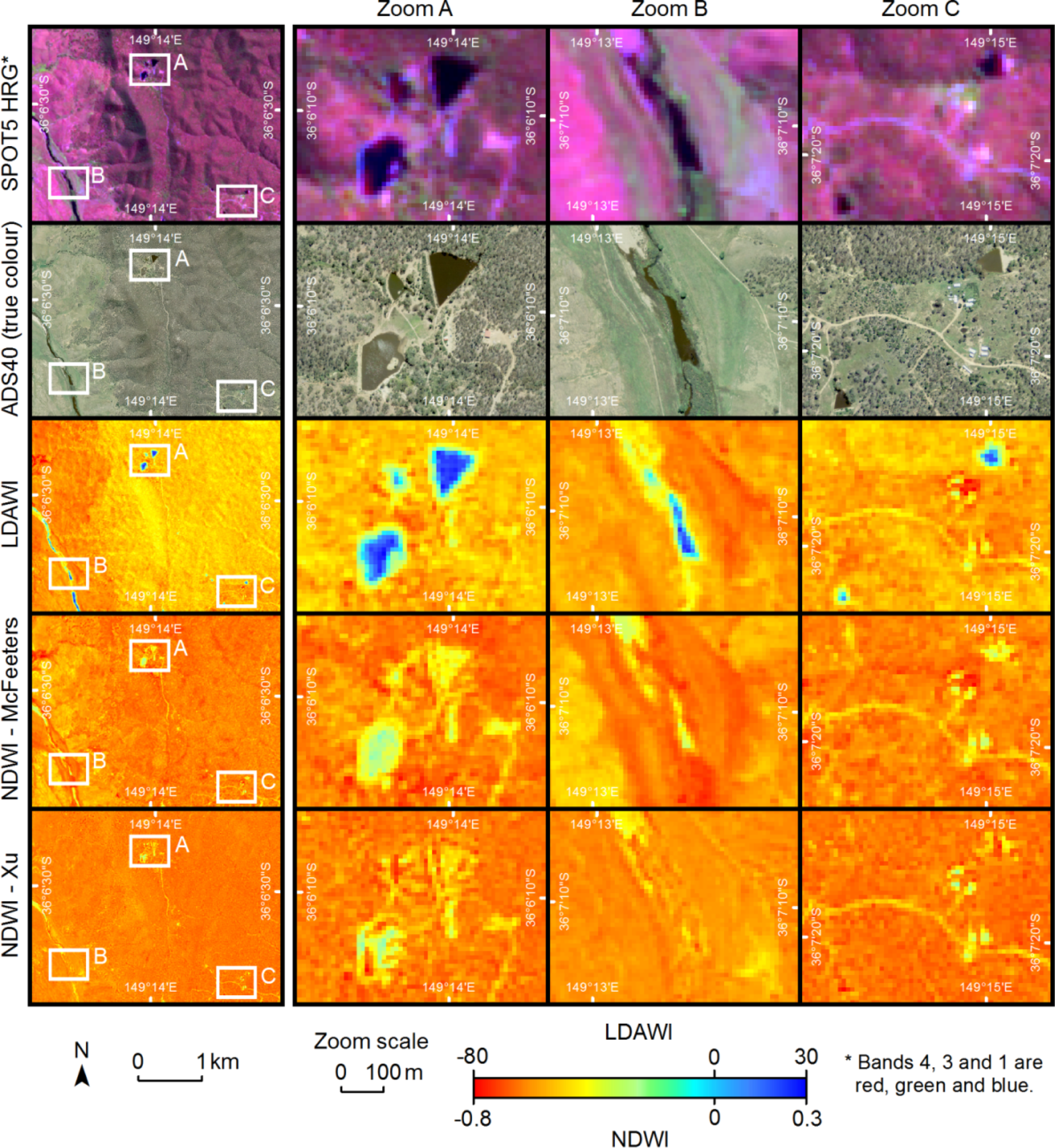
3.1. Linear Discriminant Analysis Water Index
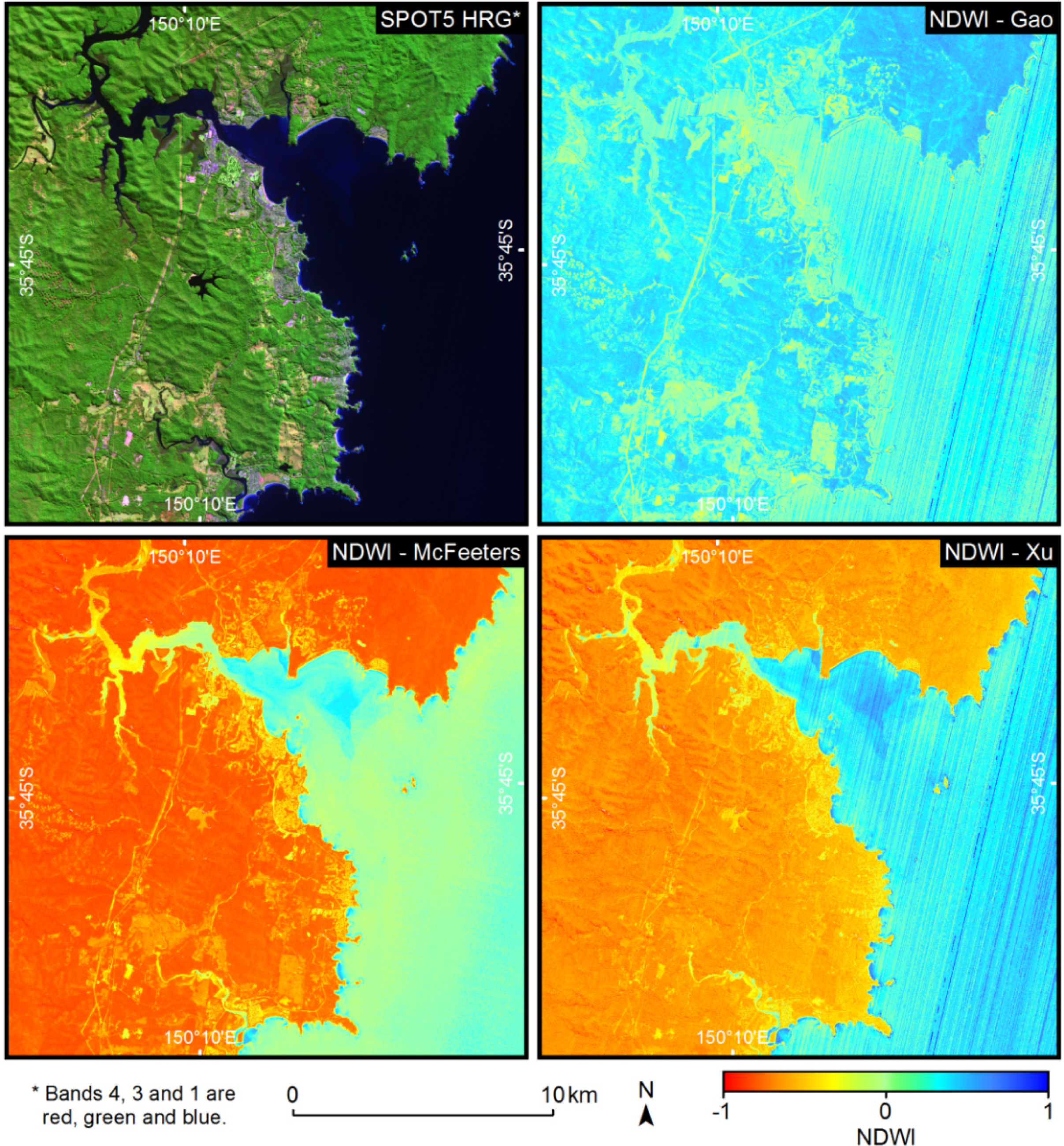
3.2. Normalized Difference Water Index
4. Discussion
5. Conclusions
Acknowledgments
Conflicts of Interest
References
- McFeeters, S.K. The use of the Normalized Difference Water Index (NDWI) in the delineation of open water features. Int. J. Remote Sens 1996, 17, 1425–1432. [Google Scholar]
- Gao, B. NDWI—A normalized difference water index for remote sensing of vegetation liquid water from space. Remote Sens. Environ 1996, 58, 257–266. [Google Scholar]
- Xu, H. Modification of Normalised Difference Water Index (NDWI) to enhance open water features in remotely sensed imagery. Int. J. Remote Sens 2006, 27, 3025–3033. [Google Scholar]
- Danaher, T.; Collett, L. Development, Optimisation and Multi-Temporal Application of a Simple Landsat Based Water Index. Proceeding of the 13th Australasian Remote Sensing and Photogrammetry Conference, Canberra, ACT, Australia, 20–24 November 2006.
- Murray, N.J.; Phinn, S.R.; Clemens, R.S.; Roelfsema, C.M.; Fuller, R.A. Continental scale mapping of tidal flats across east asia using the Landsat archive. Remote Sens 2012, 4, 3417–3426. [Google Scholar]
- McFeeters, S.K. Using the Normalized Difference Water Index (NDWI) within a geographic information system to detect swimming pools for mosquito abatement: A practical approach. Remote Sens 2013, 5, 3544–3561. [Google Scholar]
- Pai, N.; Saraswat, D. A geospatial tool for delineating streambanks. Environ. Model. Softw 2013, 40, 151–159. [Google Scholar]
- Campos, J.C.; Sillero, N.; Brito, J.C. Normalized Difference Water Indexes have dissimilar performances in detecting seasonal and permanent water in the Sahara-Sahel transition zone. J. Hydrol. 2012, 464–465, 438–446. [Google Scholar]
- Soti, V.; Tran, A.; Bailly, J.S.; Puech, C.; Seen, D.L.; Bégué, A. Assessing optical earth observation systems for mapping and monitoring temporary ponds in arid areas. Int. J. Appl. Earth Obs. Geoinf 2009, 11, 344–351. [Google Scholar] [Green Version]
- Li, W.; Du, Z.; Ling, F.; Zhou, D.; Wang, H.; Gui, Y.; Sun, B.; Zhang, X. A comparison of land surface water mapping using the Normalized Difference Water Index from TM, ETM+ and ALI. Remote Sens 2013, 5, 5530–5549. [Google Scholar]
- Zhao, D.; Lv, M.; Jiang, H.; Cai, Y.; Xu, D.; An, S. Spatio-temporal variability of aquatic vegetation in Taihu Lake over the past 30 years. PLoS One 2013, 8, e66365. [Google Scholar]
- Davranche, A.; Lefebvre, G.; Poulin, B. Wetland monitoring using classification trees and SPOT-5 seasonal time series. Remote Sens. Environ 2010, 114, 552–562. [Google Scholar] [Green Version]
- Poulin, B.; Davranche, A.; Lefebvre, G. Ecological assessment of phragmites australis wetlands using multi-season SPOT-5 scenes. Remote Sens. Environ 2010, 114, 1602–1609. [Google Scholar]
- Shook, K.; Pomeroy, J.W.; Spence, C.; Boychuk, L. Storage dynamics simulations in prairie wetland hydrology models: Evaluation and parameterization. Hydrol. Process 2013, 27, 1875–1889. [Google Scholar]
- Crist, E.P.; Cicone, R.C. A physically-based transformation of Thematic Mapper data—The TM tasseled cap. IEEE Trans. Geosci. Remote Sens 1984, 22, 256–263. [Google Scholar]
- Ouma, Y.O.; Tateishi, R. A water index for rapid mapping of shoreline changes of five east African rift valley lakes: An empirical analysis using Landsat TM and ETM+ data. Int. J. Remote Sens 2006, 27, 3153–3181. [Google Scholar]
- Danaher, T.; Scath, P.; Armston, J.; Collett, L.; Kitchen, J.; Gillingham, S. Remote Sensing of Tree-Grass Systems: The Eastern Australian Woodlands. In Ecosystem Function in Savannas: Measurement and Modeling at Landscape to Global Scales; Hill, M.J., Hanan, N.P., Eds.; CRC Press: Boca Raton, FL, USA, 2010; pp. 175–194. [Google Scholar]
- Flood, N.; Danaher, T.; Gill, T.; Gillingham, S. An operational scheme for deriving standardised surface reflectance from Landsat TM/ETM+ and SPOT HRG imagery for eastern Australia. Remote Sens 2013, 5, 83–109. [Google Scholar]
- Farr, T.G.; Rosen, P.A.; Caro, E.; Crippen, R.; Duren, R.; Hensley, S.; Kobrick, M.; Paller, M.; Rodriguez, E.; Roth, L.; et al. The shuttle radar topography mission. Rev. Geophys. 2007. [Google Scholar] [CrossRef]
- Gallant, J.; Read, A. Enhancing the SRTM Data for Australia. Proceedings of Geomorphometry, Zurich, Switzerland, 31 August–2 September 2009.
- Geoscience Australia. 1 Second SRTM Derived Digital Elevation Models User Guide; Version 1.0; Geoscience Australia: Canberra, ACT, Australia, 2010. [Google Scholar]
- Robertson, K. Spatial transformation for rapid scan-line surface shadowing. IEEE Comp. Graph. Appl 1989, 9, 30–38. [Google Scholar]
- Albanese, D.; Merler, S.; Jurman, G.; Visintainer, R.F.C. Mlpy—High-Performance Python Package for Predictive Modeling. Available online: http://mlpy.sourceforge.net/ (accessed on 15 July 2012).
- Hastie, T.; Tibshirani, R.; Friedman, J.H. The Elements of Statistical Learning: Data Mining, Inference, and Prediction, 2nd ed; Springer: New York, NY, USA, 2009; p. 758. [Google Scholar]
- Bureau of Meteorology. Climate Data Online. Available online: http://www.bom.gov.au/climate/data (accessed on 19 September 2013).


| Parameter | Value | Predictor Variable | Value |
|---|---|---|---|
| α | 224.14 | ||
| β1 | −76.18 | x1 | ln(λgreen) |
| β2 | −18.20 | x2 | ln(λred) |
| β3 | −43.00 | x3 | ln(λNIR) |
| β4 | 96.42 | x4 | ln(λSWIR) |
| β5 | 3.79 | x5 | ln(λgreen) × ln(λred) |
| β6 | 16.28 | x6 | ln(λgreen) × ln(λNIR) |
| β7 | −6.25 | x7 | ln(λgreen) × ln(λSWIR) |
| β8 | 1.54 | x8 | ln(λred) × ln(λNIR) |
| β9 | −1.14 | x9 | ln(λred) × ln(λSWIR) |
| β10 | −12.77 | x10 | ln(λNIR) × ln(λSWIR) |
| ADS40 Image Name | ADS40 Acquisition Dates | SPOT5 HRG Acquisition Date |
|---|---|---|
| Yanco | 15 February 2008–17 February 2008 | 18 February 2008 |
| Wangaratta | 25 January 2010–25 January/2010 | 25 January 2010 |
| Wagga Wagga | 15 April 2008–17 April 2008 | 16 April 2008 |
| Mt Harris | 1 March 2008–3 March 2008 | 29 February 2008 |
| Cooma | 3 March 2011–3 March 2011 | 2 March 2011 |
| Burragorang | 31 January 2009–07 February 2009 | 06 February 2009 |
| Index | Image | Threshold | Sample Size (pixels) | Overall Accuracy (%) | Producer’s Accuracy for Water (%) | Users Accuracy for Water (%) |
|---|---|---|---|---|---|---|
| LDAWI | Yanco | −37–−1 | 400 | 100.00 | 100.00 | 100.00 |
| Wangaratta | −22–−19 | 400 | 99.75 | 99.51 | 100.00 | |
| Wagga Wagga | −9–−4 | 400 | 99.75 | 100.00 | 99.50 | |
| Mt Harris | −30–−1 | 400 | 96.00 | 100.00 | 92.00 | |
| Cooma | −36–−1 | 400 | 96.25 | 100.00 | 92.50 | |
| Burragorang | 3–4 | 400 | 98.25 | 98.96 | 97.44 | |
| Total | −10 | 2,400 | 98.17 | 99.83 | 96.51 | |
| Total, no shadows | −10 | 2,386 | 98.70 | 99.83 | 97.56 | |
| Total, no shadows | −25 | 2,386 | 98.66 | 100.00 | 97.32 | |
| NDWIMcFeeters | Yanco | −0.32–−0.31 | 400 | 99.00 | 98.50 | 99.49 |
| Wangaratta | −0.30 | 400 | 97.75 | 96.55 | 98.99 | |
| Wagga Wagga | −0.31–−0.29 | 400 | 96.75 | 95.50 | 97.95 | |
| Mt Harris | −0.33 | 400 | 87.25 | 75.00 | 96.50 | |
| Cooma | −0.54 | 400 | 78.25 | 64.86 | 84.51 | |
| Burragorang | −0.26–−0.24 | 400 | 98.75 | 97.40 | 100.00 | |
| Total | −0.31 | 2,400 | 88.88 | 79.90 | 96.57 | |
| Total, no shadows | −0.31 | 2,386 | 88.81 | 79.88 | 96.57 | |
| NDWIXu | Yanco | −0.45–−0.44 | 400 | 99.75 | 99.50 | 100.00 |
| Wangaratta | −0.38–−0.27 | 400 | 97.75 | 96.55 | 98.99 | |
| Wagga Wagga | −0.46 | 400 | 95.75 | 94.00 | 97.41 | |
| Mt Harris | −0.44 | 400 | 94.25 | 94.57 | 93.05 | |
| Cooma | −0.59 | 400 | 71.75 | 60.00 | 74.00 | |
| Burragorang | −0.43–−0.38 | 400 | 98.25 | 97.92 | 98.43 | |
| Total | −0.45 | 2,400 | 91.25 | 85.91 | 95.60 | |
| Total, no shadows | −0.45 | 2,386 | 91.24 | 85.90 | 95.69 | |
© 2013 by the authors; licensee MDPI, Basel, Switzerland This article is an open access article distributed under the terms and conditions of the Creative Commons Attribution license ( http://creativecommons.org/licenses/by/3.0/).
Share and Cite
Fisher, A.; Danaher, T. A Water Index for SPOT5 HRG Satellite Imagery, New South Wales, Australia, Determined by Linear Discriminant Analysis. Remote Sens. 2013, 5, 5907-5925. https://doi.org/10.3390/rs5115907
Fisher A, Danaher T. A Water Index for SPOT5 HRG Satellite Imagery, New South Wales, Australia, Determined by Linear Discriminant Analysis. Remote Sensing. 2013; 5(11):5907-5925. https://doi.org/10.3390/rs5115907
Chicago/Turabian StyleFisher, Adrian, and Tim Danaher. 2013. "A Water Index for SPOT5 HRG Satellite Imagery, New South Wales, Australia, Determined by Linear Discriminant Analysis" Remote Sensing 5, no. 11: 5907-5925. https://doi.org/10.3390/rs5115907