Article

Evaluation of the Effects of Soil Layer Classification in the Common Land Model on Modeled Surface Variables and the Associated Land Surface Soil Moisture Retrieval Model

1
University of Chinese Academy of Sciences, Beijing 100049, China
2
ICube, UdS, CNRS, Boulevard Sebastien Brant, BP10413, Illkirch 67412, France
3
Key Laboratory of Agri-Informatics, Ministry of Agriculture/Institute of Agricultural Resources and Regional Planning, Chinese Academy of Agricultural Sciences, Beijing 100081, China
*
Author to whom correspondence should be addressed.
Remote Sens. 2013, 5(11), 5514-5529; https://doi.org/10.3390/rs5115514
Submission received: 23 August 2013 / Revised: 15 October 2013 / Accepted: 15 October 2013 / Published: 28 October 2013
(This article belongs to the Special Issue Hydrological Remote Sensing)

Abstract

:
Land surface soil moisture (SSM) is crucial in research and applications in hydrology, ecology, and meteorology. A novel SSM retrieval model, based on the diurnal cycles of land surface temperature (LST) and net surface shortwave radiation (NSSR), has recently been reported. It suggests a promising avenue for the retrieval of regional SSM using LST and NSSR derived from geostationary satellites in a future development. As part of a further improvement of previous work, effects of soil layer classification in the Common Land Model (CoLM) on modeled LST, NSSR and the associated SSM retrieval model in particular, have been evaluated. To address this issue, the soil profile has been divided in to three layers, named upper layer (0–0.05 m), root layer (0.05–1.30 m) and bottom layer (1.30–2.50 m). By varying the number of soil layers with the three layer zones, nine different soil layer classifications have been performed in the CoLM to produce simulated data. Results indicate that (1) modeled SSM is less sensitive to soil layer classification while modeled LST and NSSR are sensitive, especially under wet conditions and (2) the simulated data based SSM retrieval model is stable for a fixed upper layer with varying classifications of root and bottom layers. It also concludes an optimal soil layer classification for the CoLM while producing simulated data to develop the SSM retrieval model.

1. Introduction

With the presentation of the physical processes, initialization of underlying surface conditions and driven by atmospheric forcing data, the land surface model (LSM) is capable of describing the water budget, energy exchange and even the carbon or nitrogen cycle across the land-atmosphere interface by simulation [14]. Generally, a spin-up process is needed to make the model reach its steady-state solutions in response to an arbitrary initial condition [5,6]. The output data after spin-up process are analyzed or validated using observed values. Another use of the LSM is to simulate data with various underlying surfaces and atmospheric conditions in case such observation are not available. Subsequently models for land surface variable retrieval are developed [79]. In these situations, the initial datasets of underlying surfaces, including the surface soil moisture (SSM), soil type and land cover type, etc., are used to generate simulated data on several discrete cloud-free days under given atmospheric conditions [7]. Obviously, as only the atmospheric conditions of several individual cloud-free days are available in these cases, the spin-up process is usually not used to make the model state variables (e.g., soil moisture, surface temperature, latent heat, and net radiation) approach their equilibriums, hence, the simulated data are not only dependent on the representation of physical processes in the LSM, but also greatly affected by the soil layer classification in which the soil properties are specified [10].
In previous studies, the effects of soil layer classification on modeled surface variables have been evaluated using hydrological models with one or two soil layers [1114] to complicated land surface process models with multiple-layers [10,15]. More specifically, simulated surface variables (e.g., soil moisture variability, fluxes of energy and runoff) have been found to be significantly determined by the variation in soil depth [16,17]. However, the previous studies mainly focus on the evaluation of simulated data with different soil layer classifications. Associated models developed from LSM simulated data have been less reported on. In recent studies, Leng et al. [7] and Zhao et al. [9] reported on their SSM retrieval models that based on simulated land surface temperature (LST) and net surface shortwave radiation (NSSR) obtained with the Common Land Model (CoLM) and the Community Noah Land-surface Model, respectively. Analogous to the development of the SSM retrieval models, the two LSMs were used to produce simulated data with various underlying surfaces for each given atmospheric condition. In their studies, the soil layers were reclassified to obtain a first layer with a depth of 5 cm to enable the association with LST responses [79]. Different LSMs were originally developed with different numbers of soil layers and soil depths [18,19], and changing the number of vertical layers of which the thickness of the individual layers can potentially influence simulated land surface states and fluxes through soil water [15]. Hence, it is difficult to determine which soil layer classification is the best, and it is necessary to evaluate the effects of soil layer classification on the modeled surface variables and more importantly, the effect on the associated retrieval model for surface variables.
Within this context, the objective of the study presented in this paper, is to evaluate the effects of soil layer classification in the CoLM on simulated diurnal cycles of LST and NSSR and especially the impact on the associated SSM retrieval model by Leng et al. [7]. Furthermore, this study aims to develop an optimal soil layer classification for CoLM while producing simulated data to develop the SSM retrieval model.

2. Method

2.1. CoLM Overview

The CoLM is a state-of-the-art land surface model developed for use in climate studies [20]. A detailed description of the model is provided by Dai et al. [21], where model initialization, physical parameterizations as well as offline model testing are presented. CoLM has been developed based on the best features of three existing LSMs, including the Biosphere-Atmosphere Transfer Scheme (BATS) [22], the LSM developed by Bonan [23], and the 1994 version of the Chinese Academy of Sciences Institute of Atmospheric Physics LSM (IAP94) [24]. Until now, the model performances have been validated in sites with extensive field data [19]. Driven by atmospheric forcing data, in total 92 variables with a preset time resolution are the outputs of CoLM.

2.2. SSM Retrieval Model

Leng et al. [7] reported a bare SSM retrieval model based on simulated diurnal LST and NSSR cycles. In the development of the SSM retrieval model, CoLM has been selected to produce all simulated data for different underlying surfaces and atmospheric conditions. With the comparison and validation for both simulated data and field measurements based on two AmeriFlux site datasets, the SSM retrieval model is believed to be capable of estimating daily average SSM for bare soils. The SSM retrieval model can be written as:
SSM = n 1 x 0 + n 2 y 0 + n 3 a + n 4 θ + n 0
where SSM is the daily average SSM (m3/m3), and x0, y0, a and θ are the ellipse parameters from an elliptical relationship between diurnal LST and NSSR cycles, representing the ellipse center horizontal coordinate, ellipse center vertical coordinate, semi-major axis and rotation angle, respectively. ni (i = 0, 1, 2, 3, 4) are the model parameters (m3/m3). The SSM retrieval model has been proven to be independent of soil type, and the model parameters ni (i = 0, 1, 2, 3, 4) are dependent on atmospheric conditions only for each individual cloud-free day. In general, the model parameters ni (i = 0, 1, 2, 3, 4) can be obtained by either field measurements or LSM simulation.

2.3. Experimental Design

For the soil profile in the original CoLM, the soil depth of 10 unevenly vertical spaced soil layers is expressed as an exponential function of layer index j. The depth zj of the jth soil layer is defined as:
z j = 0.025 ( e j 2 0.25 1 ) for ( j = 1 , 2 , ... , 10 )
where j is the layer index, increasing from top soil to soil bottom.
To better evaluate the effects of soil layer classification on modeled diurnal LST and NSSR cycles, and more importantly, the associated SSM retrieval model of Leng et al. [7], the soil profile has been divided into three layer zones named: upper layer (0–0.05 m), root layer (0.05–1.30 m) and bottom layer (1.30–2.50 m). The SSM is considered to be the moisture in the upper layer until a depth of 5 cm. The number of soil layers in the upper layer varies from one to three, while for the bottom layer from one to five. The total number of soil layers is fixed to 10. The final result of soil depth (m) in function of the soil layer index (labeled with j = 1, 2, …, 10) for nine soil layer reclassifications (labeled from I to IX) are shown in Table 1.
In addition to the soil layer reclassification, land cover type was set to Barren or Sparely Vegetated according to the United States Geological Survey (USGS) vegetation categories which have been implemented in CoLM. Since the SSM retrieval model is for bare soils, the fractional vegetation cover has been set equal to 0. In total, 12 typical soil types (according to the Food and Agriculture Organization (FAO) classification), have been implemented to represent different soil types. For each soil type, 10 intervals of initial SSM range from a minimum value (around the wilting point) to maximum (around the saturated moisture content). Table 2 shows the soil types and their corresponding moisture ranges.
Finally, meteorological data (Table 3) for eight cloud-free days ranging from early April to late October for the year 2001 at the Bondville site (40.0062°N, 88.2904°W) were used as input for CoLM to produce a simulated dataset.

3. Result and Discussion

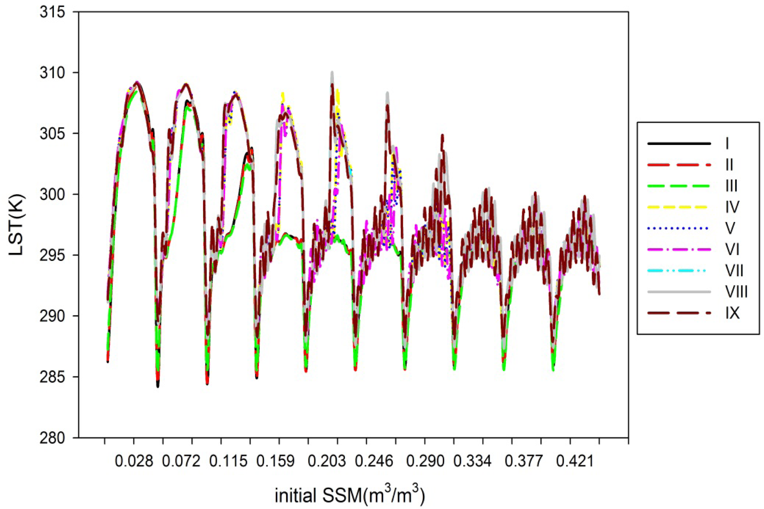
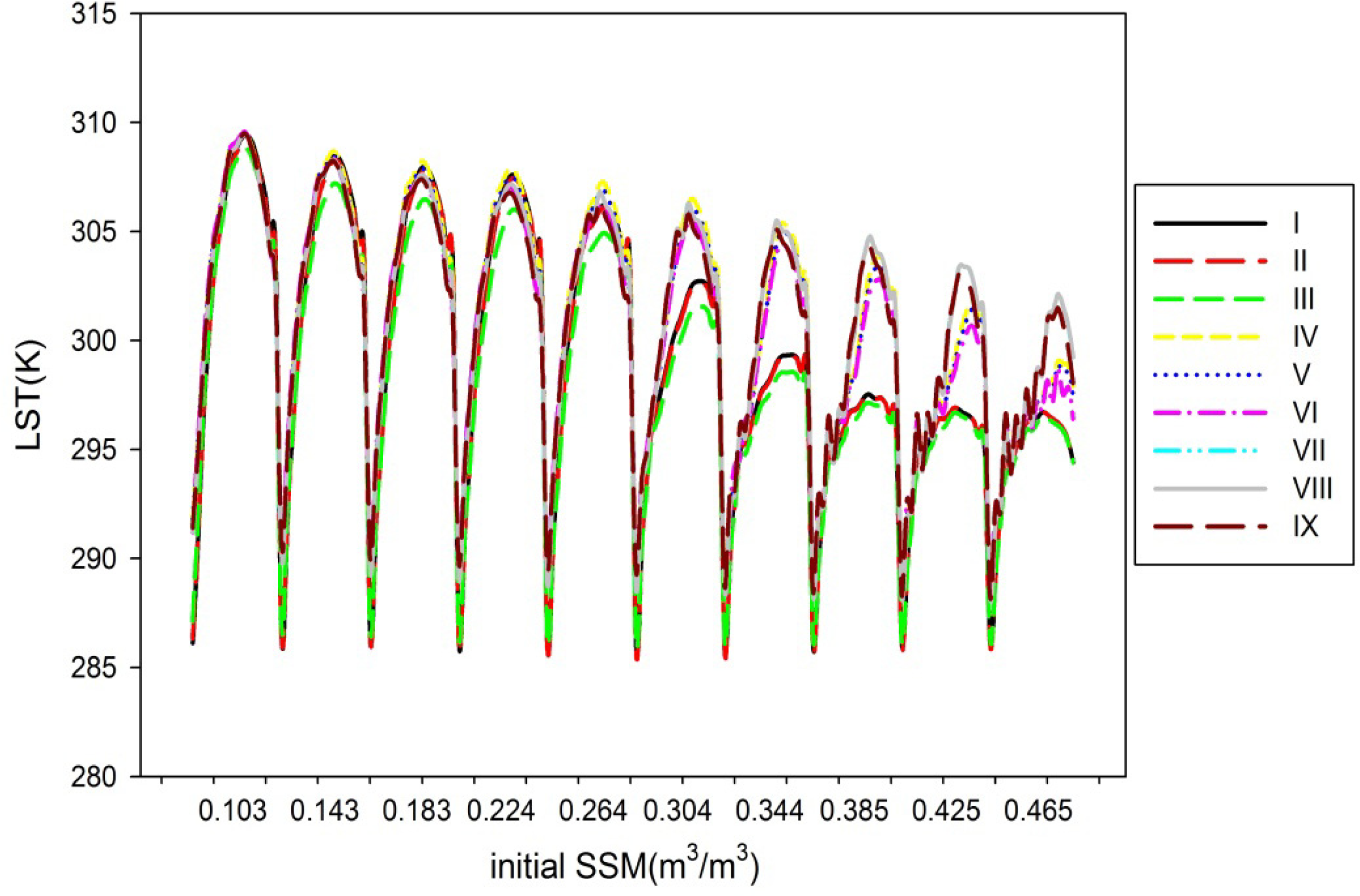
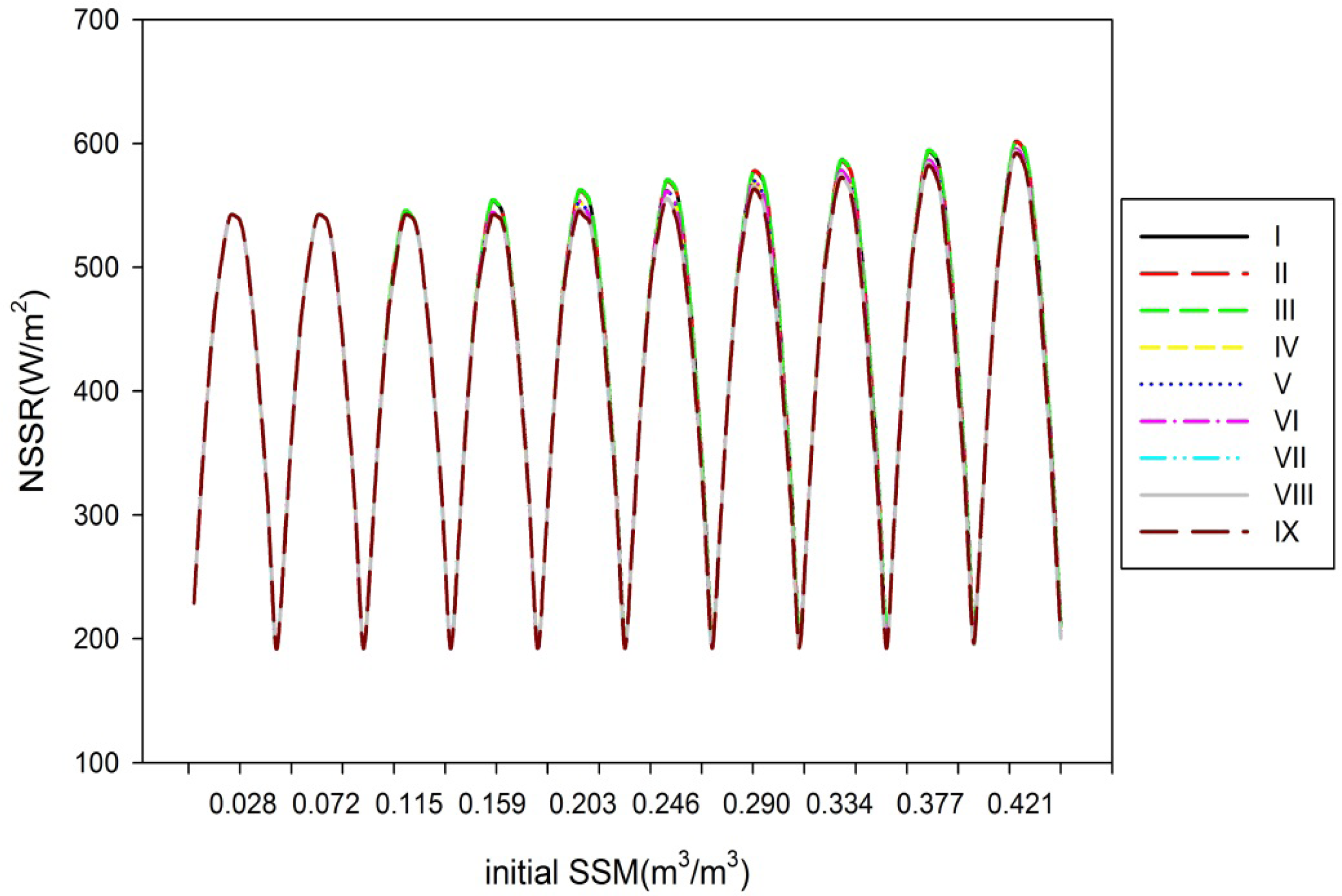
3.1. Simulated Land Surface Variables with Different Soil Layer Classifications

Two typical soils (see Table 2) Loamy Sand and Clay Loam, with appreciably different hydraulic characteristics, have been selected to evaluate the effects of soil layer classification on simulated diurnal LST and NSSR cycles as well as daily average SSM. When taking DOY 274 as an example, Figures 1 and 2 depict the diurnal curves of LST and NSSR for the nine soil layer classifications with Loamy Sand, respectively, with an initial SSM varying from 0.028 to 0.421 m3/m3. Similarly, Figures 3 and 4 depict results for Clay Loam with an initial SSM ranging from 0.103 to 0.465 m3/m3. As illustrated by Figures 1 and 3, with an increasing initial SSM, the differences of diurnal LST cycles between the nine soil layer classifications become more significant, especially when the initial SSM exceeds field capacity. Note that in that case the field capacity of Loamy Sand and Clay Loam are about 0.13 m3/m3 and 0.34 m3/m3, respectively. Results indicate as well, that the modeled diurnal LST cycle is quite sensitive to differences in soil layer classification. For the diurnal NSSR cycles, both of the soils exhibit similar characteristics according to Figures 2 and 4. Maximum NSSR increases gradually with increasing initial SSM. However, the impact of different soil layers classifications appears gradually, while the initial SSM exceeds the field capacity for the two soil types.
Figure 5 depicts scatter plots of simulated daily average SSM and the initial SSM for the two soils. The figure illustrates that simulated daily average SSM is not sensitive to soil layer classification. It is only dependent on the initial SSM and soil type for a given atmospheric conditions.

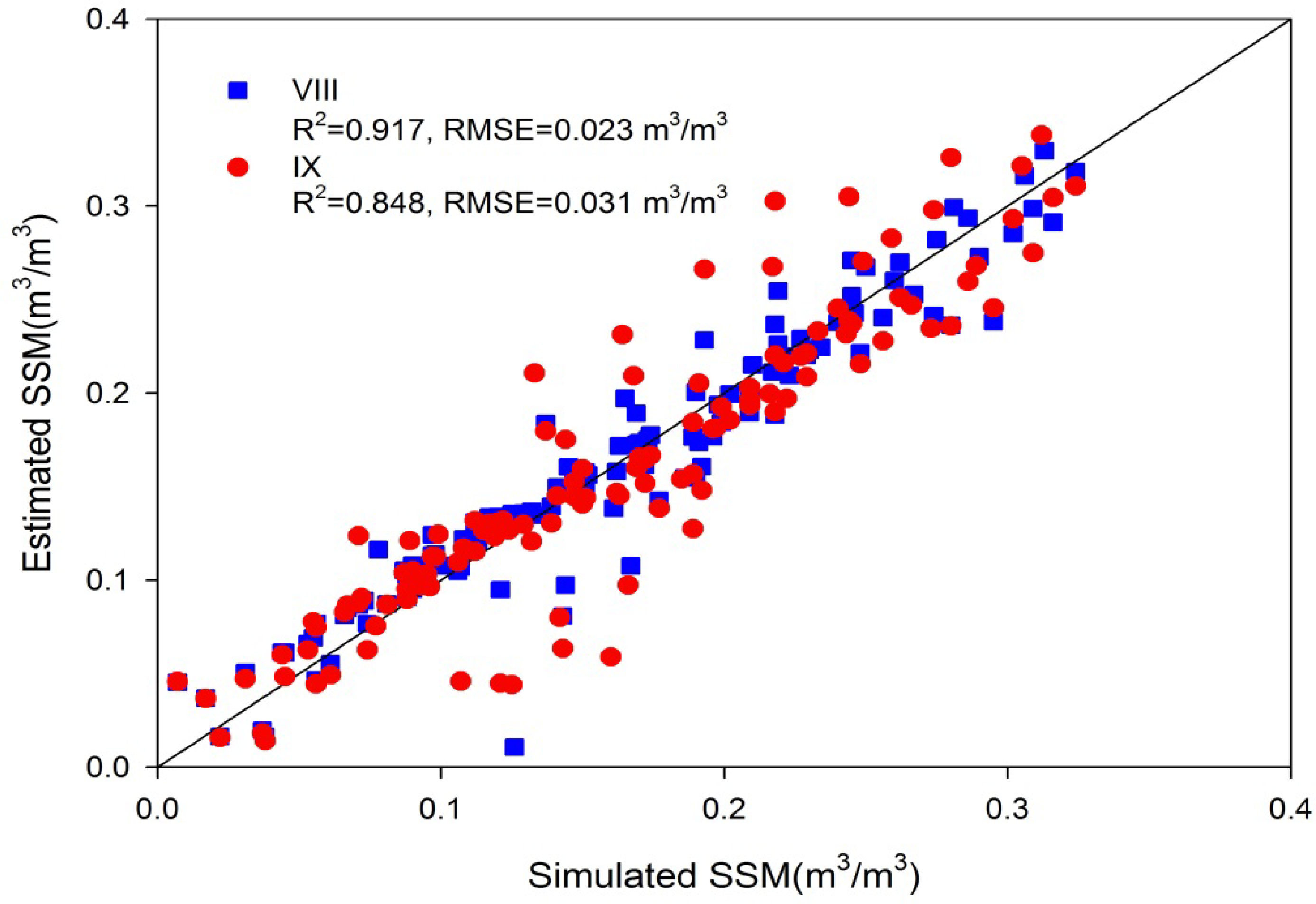
3.2. Impact of Soil Layer Classification on the SSM Retrieval Model

According to the results described in the previous section, diurnal LST and NSSR cycles respond differently to different soil layer classifications for a given atmospheric conditions. Hence, the model parameters ni (i = 0, 1, 2, 3, 4) of the SSM retrieval model in Equation (1) probably vary according to the different soil layer classifications. Table 4 shows the SSM retrieval model parameters ni (i = 0, 1, 2, 3, 4) for each soil layer classification for DOY 274.
Similar as in Table 4, the first layer of the soil classifications I, II and III is the upper layer (0–5 cm). Both the number and classification of the root layer and bottom layer are different. For classifications IV, V and VI, the upper layer has been divided in to two soil layers. The upper layer of classifications VII, VIII and IX is composed of three soil layers. It is obvious that the model parameters ni (i = 0, 1, 2, 3, 4) and the accuracies vary quite differently in function of the soil layer classifications. Hence, it is difficult to determine which soil layer classification is optimal when applying simulated data for the development of the SSM retrieval model. It is also necessary to evaluate the impact of the model parameters ni (i = 0, 1, 2, 3, 4) on the retrieval accuracy of SSM.
To achieve this objective, we ordered classification I, II and III in to group 1, IV, V and VI to Group 2, and VII, VIII and IX to Group 3. Firstly, we assessed the impact of soil layer classification on the retrieval of SSM for each group. The model parameters ni (i = 0, 1, 2, 3, 4) for soil layer classification II were applied for I and III in the Group 1, respectively. Figure 6 illustrates the results. Clearly this figure shows that the accuracy of I and III does not decrease significantly, when using the model parameter ni (i = 0, 1, 2, 3, 4) for soil classification II. This indicates that the modeled ni (i = 0, 1, 2, 3, 4) for the soil layer classification II is suitable to estimate SSM with soil layer classifications I and III as well. Similar results have been obtained for the other two groups as well. In Figure 7, SSM of classification V and VI are estimated with the model parameters ni (i = 0, 1, 2, 3, 4) for the soil layer classification IV, while Figure 8 depicts the results of the retrieval of SSM in soil layer classification VII and VIII with model parameters ni (i = 0, 1, 2, 3, 4) for the soil layer classification IX.
From above results, it can be concluded that the simulated data based SSM retrieval model is stable with a fixed upper layer and variable root and bottom soil layer classifications. Since the accuracy of the SSM retrieval model shown in the soil layer classification I, II and III is stable, with a relatively higher accuracy compared with the other classifications, they are suggested to be a reasonable choice in this study.
Furthermore, we applied the model parameters ni (i = 0, 1, 2, 3, 4) in the soil layer classification II to estimate SSM with soil layer classification VII. This enabled us to investigate the impact of different upper layer classifications on the SSM retrieval model. Figure 9 depicts the result. Clearly, SSM is over-estimated in this situation, though the coefficient of determination reaches a relatively high level (R2 = 0.856). It was also apparent that different upper layer classification greatly affects the SSM retrieval model. Thus, it is essential to determine a suitable soil layer classification for the CoLM while producing simulated data to develop the SSM retrieval model.

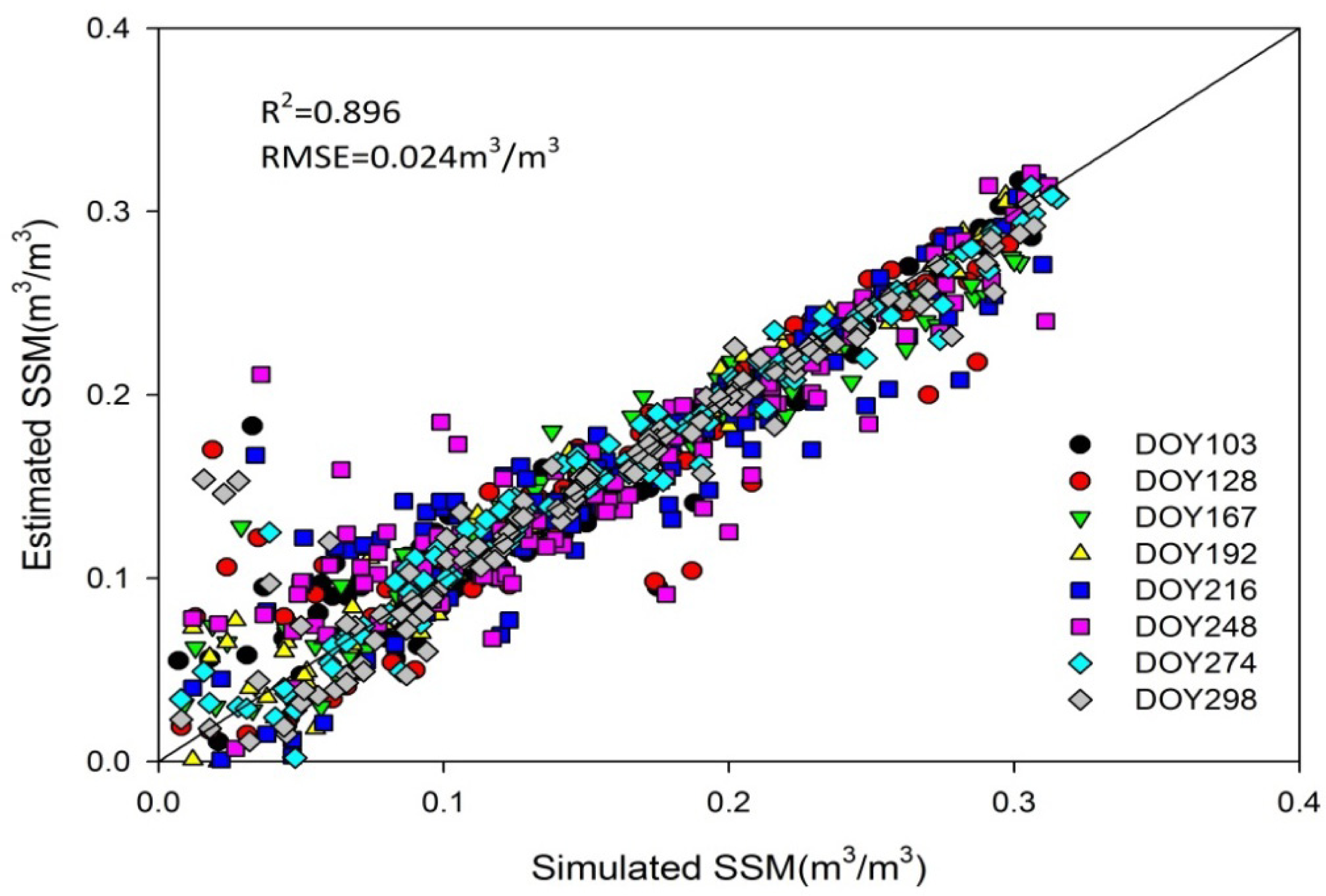
3.3. SSM Retrieval for Cloud-Free Days

Since above results are based on data simulated for DOY 274, to determine the general applicability of the soil layer classifications to the SSM retrieval model, we conducted the nine soil layer classifications further for the CoLM to produce simulated data for the other seven cloud-free days. Subsequently the results with the simulated data are then evaluated. Figure 10 illustrates the results of the comparison of R2 and RMSE for the nine soil layer classifications with the selected eight cloud-free days. According to the results, the RMSE for all the situations was within 0.05 m3/m3, and most of the R2 exceeded 0.7.
In Summary, soil layer classifications I, II and III were the best for these eight days with average coefficient of determination, R2 reaching values of 0.890, 0.896 and 0.895, respectively, while the corresponding RMSEs were 0.025 m3/m3, 0.024 m3/m3 and 0.025 m3/m3, respectively. In addition, it is believed that classifying the root layer more detail than the bottom layer is reasonable, giving attention to the fact that the root layer affects the upper layer more than the bottom layer. According to cited results, soil layer classification II is suggested to be an optimal choice in this study for the production of simulated data in CoLM enabling the development of SSM retrieval model.
With soil layer classification II, a comparison of daily average SSM estimated with Equation (1) with the simulated average SSM for each of the eight cloud-free days is shown in Figure 11. As seen from the figure, R2 reached 0.896 and RMSE was approximately 0.024 m3/m3, which indicated that the soil layer classification was suitable in this study.

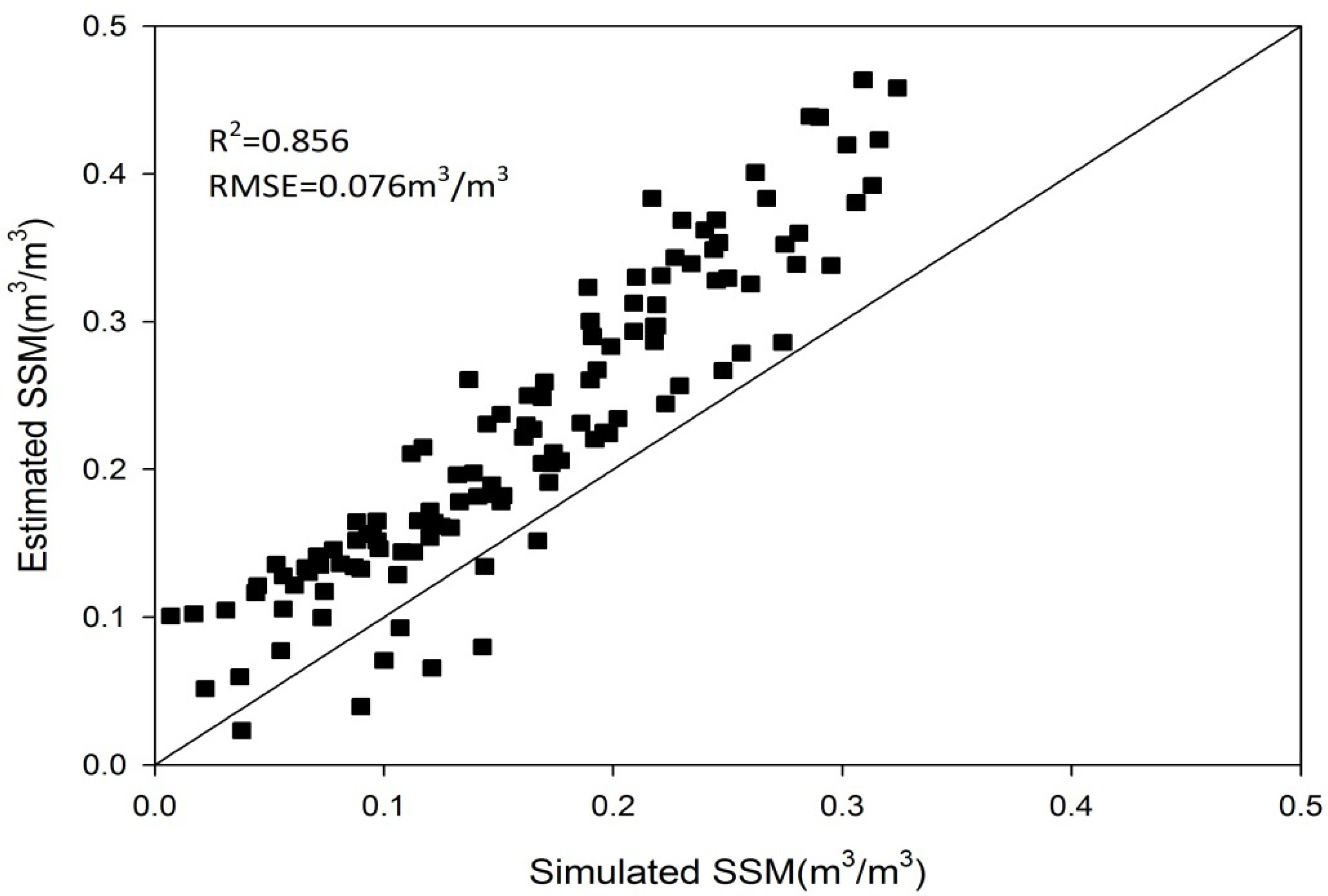
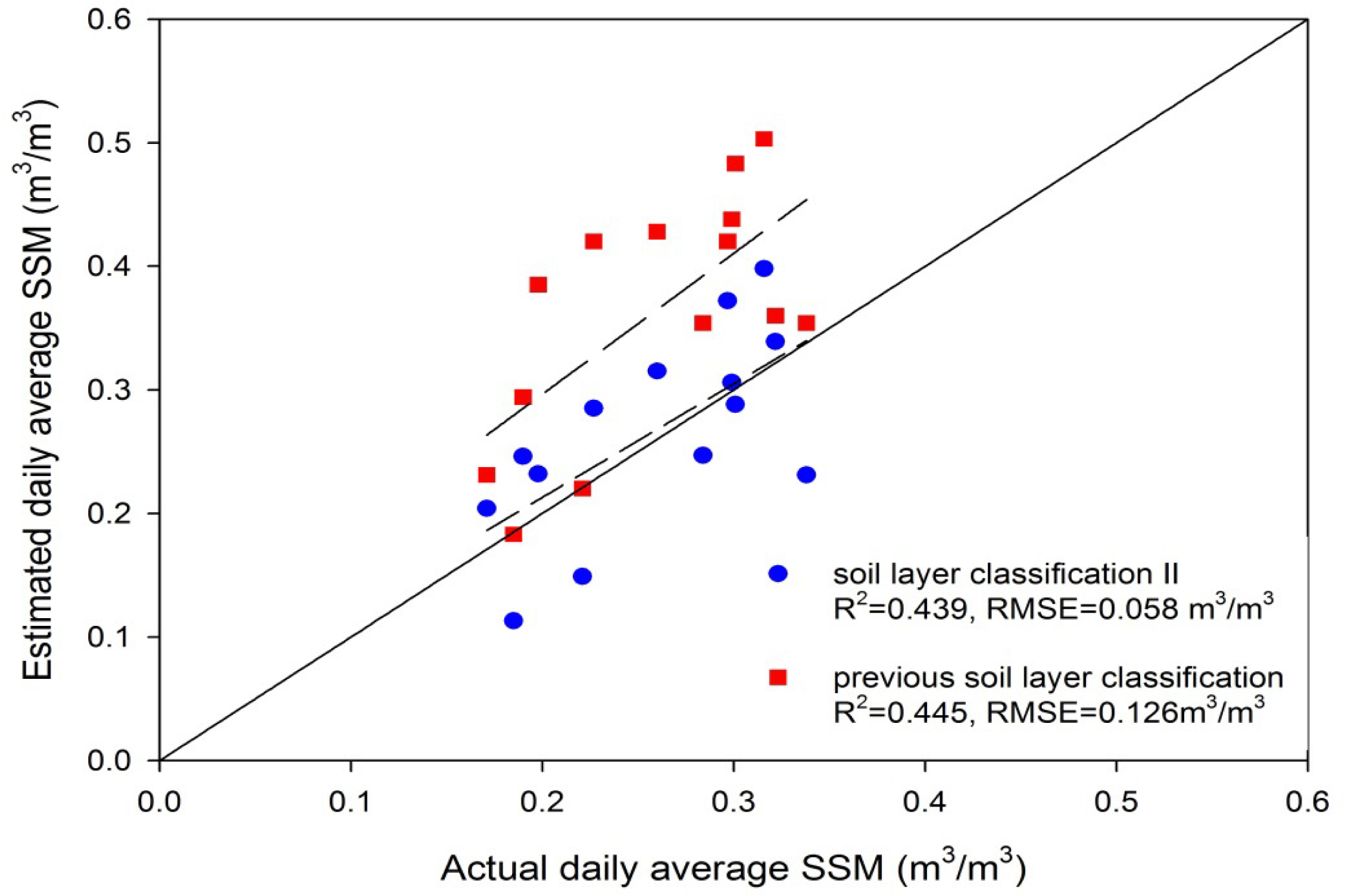
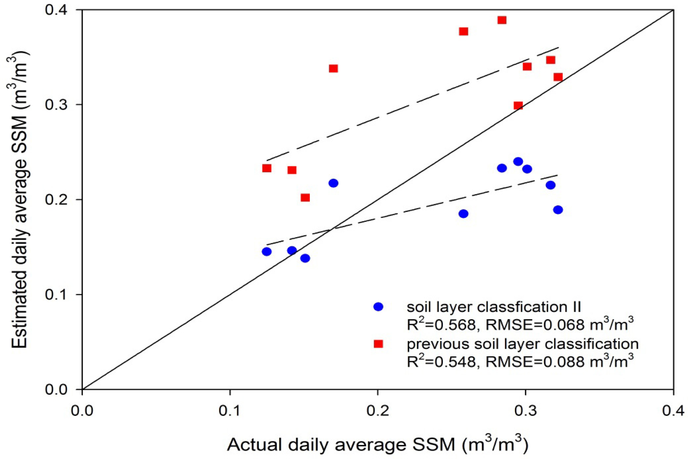
3.4. Validation with Measured Data

To further assess the capacities of the soil classification II in the SSM retrieval, a preliminary validation was performed using the two AmeriFlux field measurements, Bondville site (40.0062°N, 88.2904°W) and Bondville Companion site (40.0061°N, 88.2918°W). Validation with the field measurements of these two sites has also been stated in the previous study by Leng et al. [7]. In this study, daily average SSM were obtained with the soil layer classification II. Comparisons of the estimated SSM versus the actual SSM for the two sites are described in Figures 12 and 13, respectively. As seen from the results of Bondville site in Figure 12, coefficient of determination (R2 = 0.439) for the soil layer classification II is quite close to that of the previous study (R2 = 0.445). However, compared with the previous study, RMSE for the soil layer classification II significantly decreases from 0.126 m3/m3 to 0.058 m3/m3, which indicates that the soil layer classification II is better than the previous soil layer classification. Similar results can be found in Bondville Companion site as well according to Figure 13. In Bondville Companion site, R2 of the two soil layer classifications are approximately equal. Compared with the previous soil layer classification, RMSE for the soil layer classification II decreases from 0.088 m3/m3 to 0.068 m3/m3.

4. Conclusions

SSM is a key land surface variable in many applications and environmental studies. Various studies have been introduced to retrieve SSM or SSM related surface variables [2528]. Since LSM is capable of simulating the components of the water budget, energy exchange and other surface fluxes with acceptable accuracy, it plays an increasingly important role in obtaining surface variables at various scales. Especially, it is an effective tool providing simulated data for the development of land surface variable retrieval models when observed datasets are not available. Based on simulated data, we evaluated the impact of soil layer classification on SSM retrieval model proposed by Leng et al. [7]. Results indicate that simulated LST and NSSR are sensitive to soil layer classifications especially in wet conditions. However, the variation of soil layer classification has little influence on simulated daily average SSM. Furthermore, by varying the number of soil layers for the upper, root and bottom layers, it was found that the SSM retrieval model is stable when fixing the upper layer. It is concluded as well, that soil layer classification II was the best choice in this study. The upper layer was set to 0–5 cm with the number of root and bottom layers equaling six and three, respectively. Finally, soil layer classification II was applied using CoLM to assess estimated SSM for other cloud-free days. The coefficient of determination reached a value of 0.896 and the RMSE was approximately 0.024 m3/m3. This indicates that soil layer classification II is suitable for CoLM to produce simulated data, and hence, to develop the SSM retrieval model. With a preliminary validation with field measurement, it is believed that soil layer classification II is better than the previous soil layer classification.
This study assessed the impact of soil layer classifications with CoLM on modeled diurnal LST and NSSR cycles and the associated SSM retrieval model. An optimal soil layer classification has been selected for CoLM in the development of the SSM retrieval model. However, it has to be noted that the present study and the SSM retrieval model are based on bare soil. To be able to make more general conclusions, the development of the SSM retrieval model for vegetated surfaces and the assessment of the soil layer classification impact on the SSM retrieval model must be addressed as ongoing work.

Acknowledgments

The work described in this publication has been supported in part by the National Nature Science Foundation of China under Grant No. 41271379, partly supported by the CAS (Chinese Academy of Sciences) Action-Plan for West Development under Grant No. KZCX2-XB3-15, and also partly supported by the Exploratory Forefront Project for the Strategic Science Plan in IGSNRR, CAS under grant No. 2012QY006. The authors also thank the FLUXNET for supplying data and advice. Pei Leng is financially supported by China Scholarship Council for his stay in ICube, Strasbourg, France.

Conflicts of Interest

The authors declare no conflict of interest.

References

  1. Gusev, Y.M.; Nasonova, O.N. An experience of modelling heat and water exchange at the land surface on a large river basin scale. J. Hydrol 2000, 233, 1–18. [Google Scholar]
  2. Acora, V.K. Simulating energy and carbon fluxes over winter wheat using coupled land surface and terrestrial ecosystem models. Agric. For. Meteorol 2003, 118, 21–47. [Google Scholar]
  3. Gibelin, A.L.; Calvet, J.C.; Viovy, N. Modelling energy and CO2 fluxes with an interactive vegetation land surface model-Evaluation at high and middle latitudes. Agric. For. Meteorol 2008, 148, 1611–1624. [Google Scholar]
  4. Alton, P.B. From site-level to global simulation: Reconciling carbon, water and energy fluxes over different spatial scales using a process-based ecophysiological land-surface model. Agric. For. Meteorol 2013, 176, 111–124. [Google Scholar]
  5. Dickinson, R.E.; Shaikh, M.; Bryant, R; Graumlich, L. Interactive canopies for a climate model. J. Clim 1998, 11, 2823–2836. [Google Scholar]
  6. Shi, M.; Yang, Z.L.; Lawrence, D.M.; Dickinson, R.E.; Subin, Z.M. Spin-up processes in the Community Land Model version 4 with explicit carbon and nitrogen components. Ecol. Model 2013, 263, 308–325. [Google Scholar]
  7. Leng, P.; Song, X.; Li, Z.-L.; Ma, J.; Zhou, F.; Li, S. Bare surface soil moisture retrieval from the synergistic use of the optical and thermal infrared data. Int. J. Remote Sens. 2013, in press.. [Google Scholar]
  8. Zhao, W.; Li, Z.-L. Sensitivity study of soil moisture on the temporal evolution of surface temperature over bare surfaces. Int. J. Remote Sens 2013, 34, 3314–3331. [Google Scholar]
  9. Zhao, W.; Li, Z.-L.; Wu, H.; Tang, B.-H.; Zhang, X.; Song, X.; Zhou, G. Determination of bare surface soil moisture from combined temporal evolution of land surface temperature and net surface shortwave radiation. Hydrol. Process 2013, 27, 2825–2833. [Google Scholar]
  10. Martinez, J.E.; Duchon, C.E.; Crosson, W.L. Effect of the number of soil layers on a modeled surface water budget. Water Resour. Res 2001, 37, 367–377. [Google Scholar]
  11. Mahrt, L.; Pan, H. A two-layer model of soil hydrology. Bound. Layer Meteorol 1984, 29, 1–20. [Google Scholar]
  12. Hughes, D.; Sami, K. A semi-distributed, variable time interval model of catchment hydrology-structure and parameter estimation procedures. J. Hydrol 1994, 155, 265–291. [Google Scholar]
  13. Liang, X.; Lettenmaier, P.; Wood, E.; Burges, S. A simple hydrologically based model of land surface water and energy fluxes for general circulation models. J. Geophys. Res 1994, 99, 14415–14428. [Google Scholar]
  14. Lakshmi, V.; Wood, E. Diurnal cycles of evaporation using a two-layer hydrological model. J. Hydrol 1998, 204, 37–51. [Google Scholar]
  15. Gochis, D.J.; Vivoni, E.R.; Watts, C.J. The impact of soil depth on land surface energy and water fluxes in the North American Monsoon region. J. Arid Environ 2010, 74, 564–571. [Google Scholar]
  16. Wang, A.; Zeng, X.; Shen, S.; Zeng, Q.; Dickinson, R.E. Timescales of land surface hydrology. J. Hydrometeorol 2006, 7, 868–879. [Google Scholar]
  17. Meerveld, I.T.; Weiler, W. Hillslope dynamics modeled with increasing complexity. J. Hydrol 2008, 361, 24–40. [Google Scholar]
  18. Chen, F.; Jimy, D. Coupling an advanced land surface-hydrology model with the Penn State-NCAR MM5 modeling system. Mon. Wea. Rev 2001, 129, 569–585. [Google Scholar]
  19. Dai, Y.; Ji, D. The Common Land Model (CoLM) User’s Guide. 2005. Available online: http://globalchange.bnu.edu.cn/research/models (accessed on 7 July 2008).
  20. Zeng, X.; Shaikh, M.; Dai, Y.; Dickinson, R.E.; Myneni, R. Coupling of the common land model to the NCAR community climate model. J. Clim 2002, 15, 1832–1854. [Google Scholar]
  21. Dai, Y.; Zeng, X.; Dickinson, R.E.; Baker, I.; Bonan, G.; Bosilovich, M.; Denning, A.; Dirmeyer, P.; Houser, P.; Niu, G.; et al. The common land model. Bull. Amer. Meteor. Soc 2003, 8, 1013–1023. [Google Scholar]
  22. Dickinson, R.E.; Henderson-Sellers, A.; Kennedy, P.J. Biosphere-Atmosphere Transfer Scheme (BATS) Version 1e as Coupled to Community Climate Model; NCAR Technical Note NCAR/TN-387+STR; Climate and Global Dynamics Division (CGD), NCAR: Boulder, CO, USA,. 1993. Available online: http://opensky.library.ucar.edu/collections/TECH-NOTE-000-000-000-198 (accessed on 21 October 2012).
  23. Bonan, G.B. A Land Surface Model (LSM Version 1.0) for Ecological, Hydrological, and Atmospheric Studies: Technical Description and User’s Guide; NCAR Technical Note NCAR/TN-417+STR; National Center for Atmospheric Research: Boulder, CO, USA, 1996; p. 150. [Google Scholar]
  24. Dai, Y.; Zeng, Q.-C. A land surface model (IAP94) for climate studies, Part I: Formulation and validation in off-line experiments. Adv. Atmos. Sci 1997, 14, 433–460. [Google Scholar]
  25. Li, Z.-L.; Tang, R.L.; Wan, Z.; Bi, Y.; Zhou, C.; Tang, B.H.; Yan, G.; Zhang, X. A review of current methodologies for regional evapotranspiration estimation from remotely sensed data. Sensors 2009, 9, 3801–3853. [Google Scholar]
  26. Li, Z.-L.; Tang, B.H.; Wu, H.; Ren, H.; Yan, G.; Wan, Z. Satellite-derived land surface temperature: Current status and perspectives. Remote Sens. Environ 2013, 131, 14–37. [Google Scholar]
  27. Song, X.; Leng, P.; Li, X.; Li, X.; Ma, J. Retrieval of daily evolution of soil moisture from satellite-derived land surface temperature and net surface shortwave radiation. Int. J. Remote Sens 2013, 34, 3289–3298. [Google Scholar]
  28. Pierdicca, N.; Pulvirenti, L.; Bignami, C. Soil moisture estimation over vegetated terrains using multitemporal remote sensing data. Remote Sens. Environ. 2010, 114, 440–448. [Google Scholar]
Figure 1. Diurnal LST curves of Loamy Sand with initial SSM varying from 0.028 to 0.421 m3/m3. Each curve with a wave peak responds to an initial SSM value. The nine different soil layer classifications labeled from I to IX are depicted with different line styles and colors.
Remotesensing 05 05514f1
Figure 2. Diurnal NSSR curves of Loamy Sand with initial SSM varying from 0.028 to 0.421 m3/m3. Each curve with a wave peak responds to an initial SSM value. The nine different soil layer classifications labeled from I to IX are depicted with different line styles and colors as well.
Remotesensing 05 05514f2
Figure 3. Diurnal LST curves of Clay Loam with initial SSM varying from 0.103 to 0.465 m3/m3. Each curve with a wave peak responds to an initial SSM value. The nine different soil layer classifications labeled from I to IX are depicted with different line styles and colors as well.
Remotesensing 05 05514f3
Figure 4. Diurnal NSSR curves of Clay Loam with initial SSM varying from 0.103 to 0.465 m3/m3. Each curve with a wave peak responds to an initial SSM value. The nine different soil layer classifications labeled from I to IX are depicted with different line styles and colors as well.
Remotesensing 05 05514f4
Figure 5. Scatter plots of simulated daily average SSM versus initial SSM for two typical soils.
Remotesensing 05 05514f5
Figure 6. Comparison between estimated daily average SSM and simulated daily average. The model parameters ni (i = 0, 1, 2, 3, 4) for the soil layer classification II were applied to I and III to estimate daily average SSM using Equation (1).
Remotesensing 05 05514f6
Figure 7. Comparison between estimated daily average SSM and simulated daily average. The model parameters ni (i = 0, 1, 2, 3, 4) for the soil layer classification IV were applied to V and VI to estimate daily average SSM using Equation (1).
Remotesensing 05 05514f7
Figure 8. Comparison between estimated daily average SSM and simulated daily average. The model parameters ni (i = 0, 1, 2, 3, 4) for the soil layer classification VII were applied to VIII and IX to estimate daily average SSM using Equation (1).
Remotesensing 05 05514f8
Figure 9. Comparison between estimated daily average SSM and simulated daily average. The model parameters ni (i = 0, 1, 2, 3, 4) for the soil layer classification II were applied to VII to estimate daily average SSM using Equation (1).
Remotesensing 05 05514f9
Figure 10. Comparison of R2 and RMSE for the nine soil layer classifications with eight cloud-free days at Bondville in 2001.
Remotesensing 05 05514f10
Figure 11. Comparison of daily average estimated SSM using Equation (1) with simulated average SSM for each of the eight cloud-free days.
Remotesensing 05 05514f11
Figure 12. Comparison of daily average estimated SSM versus the actual daily average SSM at Bondville site.
Remotesensing 05 05514f12
Figure 13. Comparison of daily average estimated SSM versus the actual daily average SSM at Bondville Companion site.
Remotesensing 05 05514f13
Table 1. Different soil layer classifications used in CoLM.
Layer IndexIIIIIIIVVVIVIIVIIIIX
10.050.050.050.010.010.010.010.010.01
20.100.100.100.050.050.050.030.030.03
30.150.200.400.100.100.100.050.050.05
40.200.400.800.200.300.600.100.100.10
50.400.601.300.400.601.300.400.401.30
60.601.001.500.601.001.500.600.801.50
70.801.301.800.801.301.800.801.301.80
81.001.502.001.001.502.001.001.502.00
91.302.002.201.302.002.201.302.002.20
102.502.502.502.502.502.502.502.502.50
Table 2. Soil types and ranges of SSM used in the CoLM simulations.
No.Sand (%)Silt (%)Clay (%)Soil TypesRange of SSM (m3/m3)
19253Sand0.010–0.339
282126Loamy Sand0.028–0.421
3583210Sandy Loam0.047–0.434
4177013Silt Loam0.084–0.476
510855Silt0.084–0.476
6433918Loam0.066–0.439
7581527Sandy Clay Loam0.067–0.404
8105634Silty Clay Loam0.120–0.464
9323434Clay Loam0.103–0.465
1052642Sandy Clay0.100–0.406
1164747Silty Clay0.126–0.468
12222058Clay0.138–0.468
Table 3. Daily atmospheric conditions for eight cloud-free days used in CoLM simulations to enable the development of the daily average SSM retrieval model.
DOYMaximal Solar Radiation (W/m2)Average Wind Speed (m/s)Average Air Temperature (K)
1038644.05287.68
1289063.05297.25
1679183.02303.85
19210353.46298.95
2169683.20302.25
2488852.92302.65
2747742.59298.75
29869415.50281.39
Table 4. Parameters of Equation (1) for nine soil layer classifications.
No.n1n2n3n4n0R2RMSE (m3/m3)
I1.2893.1613.1040.923−2.8160.9510.018
II1.1923.2243.1140.920−2.7930.9530.017
III0.7623.5863.2640.823−2.6720.9560.017
IV−0.4163.4342.6200.454−1.6630.8990.025
V−0.3563.1192.5050.489−1.6210.8880.027
VI−0.3483.1922.5900.433−1.6060.8790.028
VII−0.4223.6552.7150.424−1.7040.9170.023
VIII−0.4193.6482.7110.426−1.7040.9170.023
IX−0.3583.0462.2860.410−1.4490.8500.031

