Article

Snow Cover Maps from MODIS Images at 250 m Resolution, Part 1: Algorithm Description

1
Institute for Applied Remote Sensing, EURAC, Viale Druso 1, I-39100 Bolzano, Italy
2
Department of Geography, Glaciology, Geomorphodynamics and Geochronology, University of Zürich-Irchel, Winterthurerstrasse 190, CH-8057 Zurich, Switzerland
3
Department of Geosciences, University of Oslo, P.O. Box 1047, Blindern, N-0316 Oslo, Norway
*
Author to whom correspondence should be addressed.
Current address: South Tyrol Healthcare Company, Via del Ronco 3, I-39100 Bolzano, Italy.
Remote Sens. 2013, 5(1), 110-126; https://doi.org/10.3390/rs5010110
Submission received: 1 November 2012 / Revised: 25 December 2012 / Accepted: 25 December 2012 / Published: 4 January 2013

Abstract

:
A new algorithm for snow cover monitoring at 250 m resolution based on Moderate Resolution Imaging Spectroradiometer (MODIS) images is presented. In contrast to the 500 m resolution MODIS snow products of NASA (MOD10 and MYD10), the main goal was to maintain the resolution as high as possible to allow for a more accurate detection of snow covered area (SCA). This is especially important in mountainous regions characterized by extreme landscape heterogeneity, where maps at a resolution of 500 m could not provide the desired amount of spatial details. Therefore, the algorithm exploits only the 250 m resolution bands of MODIS in the red (B1) and infrared (B2) spectrum, as well as the Normalized Difference Vegetation Index (NDVI) for snow detection, while clouds are classified using also bands at 500 m and 1 km resolution. The algorithm is tailored to process MODIS data received in real-time through the EURAC receiving station close to Bolzano, Italy, but also standard MODIS products are supported. It is divided into three steps: first the data is preprocessed, including reprojection, calculation of physical reflectance values and masking of water bodies. In a second step, the actual classification of snow, snow in forested areas, and clouds takes place based on MODIS images both from Terra and Aqua satellites. In the third step, snow cover maps derived from images of both sensors of the same day are combined to reduce cloud coverage in the final SCA product. Four different quality indices are calculated to verify the reliability of input data, snow classification, cloud detection and viewing geometry. Using the data received through their own station, EURAC can provide SCA maps of central Europe to end users in near real-time. Validation of the algorithm is outlined in a companion paper and indicates good performance with accuracies ranging from 94% to around 82% compared to in situ snow depth measurements, and around 93% compared to SCA derived from Landsat ETM+ images.

Graphical Abstract

1. Introduction

The snow covered area (SCA) is a key parameter for many applicative domains, such as hydrology, meteorology and climatology due to its impact on water availability and Earth radiation budget Moreover, as the snow extent is related to the water quantity to be released during the melting period, introduced as a state variable in the hydrological models, SCA data can be used to predict the water stage and provide information on risk phenomena such as flooding [1].
Satellite sensors are efficient tools to monitor snow cover extent [2,3] and various authors have demonstrated that SCA maps from optical satellite sensors can improve the prediction of the snow melt stream flow in hydrological models [1,4,5] and derived significant parameters such as the Snow Cover Duration (SCD), Snow Cover Start (SCS) and Snow Cover Melt (SCM) [6]. These derived parameters are useful to quantify the inter-annual changes in snow cover characteristics and represent a basis for future climate change studies.
SCA maps are mainly derived from optical satellite images with high temporal resolution (AVHRR, MODIS) in order to ensure daily availability and medium ground resolution. MODIS’s daily repeat time with two satellites, Terra and Aqua, multi-spectral capabilities and medium spatial resolution proved to be successful for this task at both regional and global scale [3,7]. Despite the availability and general performances of the MODIS MOD10 and MYD10 Snow product [3,812], obvious limitations affect the monitoring of local scale details and stress the need for an adapted and robust algorithm to map snow cover with the highest possible amount of spatial details. To improve the ground resolution, some authors exploit the 250 m to derive snow cover fraction information. Metsämäki et al.[13] and Malcher et al.[14] calculated the snow cover fraction based on the reflectances of red and near-IR bands, as well as the use of NDVI. The behavior of visible and near-infrared reflectances for snow in dry and wet conditions is well known [15].
Recently, some authors focused therefore on the development of methods to estimate the snow cover fraction in a 500 m MODIS pixel using the additional information of the two MODIS 250 m channels [16,17]. Sirguey et al.[16] report a mean error of 6.8% of sub-pixel snow fraction for eight pairs of synchronic MODIS/ASTER images in the Southern Alps of New Zealand.
The estimation of fractional snow cover is of interest because they represent an improvement of resolution with respect to 500 m of MODIS standard products [18]. While the fractional snow cover for MODIS MOD10A1 is derived from comparison of NDSI index with Landsat maps, other approaches as proposed by Vikhamar and Soldberg [19] are based on linear spectral unmixing. The MODSCAG (MODIS Snow Covered-Area and Grain size retrieval) algorithm uses a range of endmembers in the spectral mixing to estimate the grain size of the snow as well [20]. Methods for fractional snow cover based on spectral unmixing have proved to provide higher accuracies with respect to the empirical approaches based on NDSI [21].
Improved spatial resolution of the MODIS-based snow product is thus highly desirable and can be closer to the 100 m resolution requested for snow maps in complex terrain by the Global Climate Observing System (GCOS) [22]. For flat terrain 1 km is considered as an adequate ground resolution.
The main objective of this paper is to introduce an alternative approach to improve the MODIS-based SCA maps by exploiting only the 250 m resolution bands for snow detection. Furthermore, thanks to the availability of a satellite receiving station located near Bolzano, Northern Italy, the SCA maps covering most parts of central Europe can be delivered in near real-time (from two to four hours after the acquisitions) to the end-users.
The paper is organized as follows. In Section 2, the area of interest and the input data for the algorithm are described, while Section 3 introduces details of the snow algorithm, including information on the delivery of the products. Section 4 describes the quality indices associated to the SCA maps. Section 5 draws conclusions and proposes future developments. The validation of the algorithm that is a comparison to in situ measurements, Landsat data and the standard NASA MYD10-MOD10 SCA maps is presented in the companion paper [23].

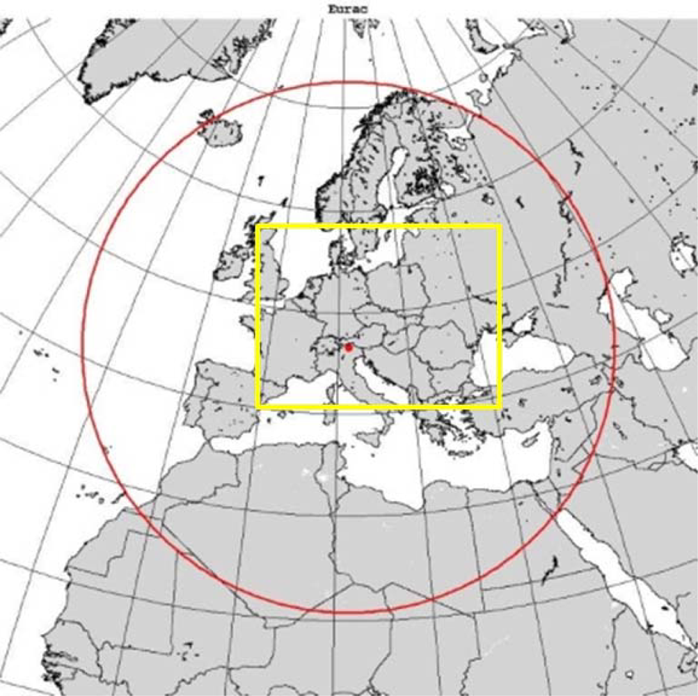
2. Study Area and Data

The proposed MODIS snow algorithm (hereafter called EURAC algorithm http://www.eurac.edu/en/research/institutes/remotesensing/default) was designed and developed to monitor snow coverage over Central Europe (42°N–51°N, 5°E–30°E) on a daily basis. This area is completely covered by the EURAC receiving station which has coverage from Iceland to the Mediterranean seas, including northern African countries (Figure 1). MODIS (or Moderate Resolution Imaging Spectroradiometer) is a key instrument aboard the Terra (EOS AM) and Aqua (EOS PM) satellites. Terra’s orbit around the earth is timed so that it passes from north to south across the equator in the morning, while Aqua passes south to north over the equator in the afternoon. Terra MODIS and Aqua MODIS are viewing the entire earth’s surface every one to two days, acquiring data in 36 spectral bands ( http://modis.gsfc.nasa.gov/about/).
The following MODIS products are used to produce the SCA maps at 250 m resolution:
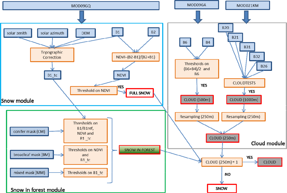
  • - MOD09GQ–MYD09GQ and MOD09GA–MYD09GA (Terra–Aqua): atmospherically corrected surface reflectance product at 250 m–500 m resolution. The 250 m resolution bands, band 1 (0.62–0.67 μm) and 2 (0.841–0.876 μm), are used to detect snow and snow in forested areas. The 500 m resolution bands, bands 4 (0.545–0.565 μm) and 6 (1.628–1.652 μm) are used to detect clouds along with 1 km resolution bands.
  • - MOD021KM–MYD021KM (Terra–Aqua): reflectance bands at 1 km resolution for cloud detection. The 1 km resolution bands are: 20 (3.660–3.840 μm), 21 (3.929–3.989 μm), 31 (10.780–11.280 μm), 32 (11.770–12.270 μm), 26 (1.360–1.390 μm).
  • - MOD03–MYD03 (Terra–Aqua): Geo-location dataset.
The algorithm is conceived to work the aforementioned products, as well as for processing by the EURAC receiving station. MODIS Products are processed by using the SeaSpace Terascan Suite version 3.3–10 that adopts the algorithm of SeaDAS v 5.1 and NASA DAAC v 4. SeaDAS itself does use IMAPP package (International MODIS/AIRS Processing Package), from CIMSS, University of Wisconsin-Madison ( http://cimss.ssec.wisc.edu/about.html).
Topographic information comes from the Shuttle Radar Topography Mission (SRTM) digital elevation model (DEM) (90 m resolution) and information on land cover (broadleaf, coniferous and mixed forest) is extracted from CORINE Land Cover 2006 ( http://sia.eionet.europa.eu/CLC2006/). For Switzerland, a forest mask developed by the Joint Research Centre (JRC) was adopted ( http://forest.jrc.ec.europa.eu/forest-mapping). The choice of the CORINE Land cover was based on the necessity to have a uniform and homogeneous land cover map which covers all the countries in the selected region of interest. Moreover, having a static map does not introduce any further processing step in the chain and this is an important aspect as the algorithm is conceived to work in real-time. However, some drawbacks emerge from the use of the CORINE Land cover map, mainly the problem of the water body change extent that will not be recognized in the procedure and the minimum map unit of 25 ha with respect to MODIS pixel of 6.25 ha. The latest can have an impact on the detection of snow in forested areas, especially in the border between snow and snow-free areas.

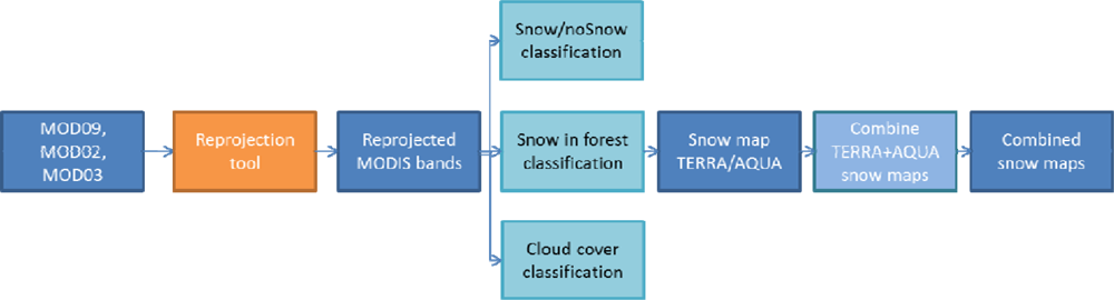
3. MODIS 250 m SCA Algorithm

The algorithm is divided into three parts (Figure 2). In the first part, the input data, is prepared for the classification (re-projection, calibration, water body masking). SCA maps of MODIS Terra and Aqua are generated in the second part, and combined in the third. The second part of the algorithm is mainly devoted to snow cover and cloud mapping and is composed of three modules. The first module is dedicated to snow detection based on the 250 m resolution MODIS bands and on Normalized Difference Vegetation Index (NDVI). The second module is related to the detection of snow in forest. The third module is devoted to the cloud detection. A detailed description of the three modules is provided in Figure 3.

3.1. Preprocessing of MODIS Data

All preprocessing steps were conceived to work both with MODIS data downloadable from NASA websites and with MODIS data received in near real-time from operating receiving stations. For this reason, part of the processing was tailored to work with the antenna facilities. In fact, the data are processed at EURAC’s processing and archiving facility conceived to deal with near real-time images, directly received through the EURAC receiving station located at Renon Peak (2,230 m). This allows ingesting the data directly from the antenna into the snow algorithm.
The re-projection tool is organized in order to be adjusted to the processing chain of the receiving station. This processor is designed to re-project all MODIS bands that are necessary to compute the SCA map over the defined area of interest into the ETRS-LAEA projection (also maps in UTM WGS824 can be available). It is able to deal with one or more granules in the same processing line. This means that the processor is able to get as inputs more granules of a single passage, for example, when the passage is split in more granules (like the Seaspace granules directly received by the receiving station).
This step includes also the calibration of the bands, thus transforming them from digital numbers (DN) to physical values, i.e., reflectances. In this case, the algorithm uses the MOD09GQ-MYD09GQ images which are already atmospherically corrected. These products are derived from Level 02 products MOD-MYD02 [24].
As topography can have a high influence on the reflectance, band 1, mainly used for snow detection, also underwent a topographic correction. This procedure is fundamental, as it reduces the effect of topography on the signal. When single bands are used, the topographic correction has to be performed in order to reduce the shadowing effects and their changes due to the seasonal cycle. This operation converts the reflectance to normalized reflectance, as if the surface was fully horizontal.
The topographic correction is a modified cosine correction, where some coefficients are empirically evaluated in order to reduce the typical over- and underestimation of the standard cosine approach [25]. The proposed approach is based on the formula:
L λ Corr = L λ ( cos θ z f ( IL ) )
where LλCorr is the corrected radiance and Lλ is the radiance at the top of the atmosphere as calculated from images, IL is the shaded relief related to the local incidence angle and θz is the sun zenith angle. The shaded relief IL varies between −1 (minimum of illumination) and 1 (maximum of illumination) and is calculated as follows:
IL = cos γ i = cos θ p cos θ z + sin θ p sin θ z cos ( φ φ a )
where θp is the slope in the considered point, θz is the sun zenith angle, φ is the sun azimuth angle and φa is the aspect in the considered point.
The function f(IL) is supposed to be linear, f(IL)=a+b*IL and the coefficients, a and b, are calculated by posing two conditions the corrected radiance has to fulfill, that is:
  • - after the correction, the areas “in light” and those “in shadow” should have the same mean radiance;
  • - the corrected radiance of areas in the correct sun illumination should remain equal to non-corrected radiance.
These areas are obtained by considering the relationship between the cosine of the sun zenith angle and the shaded relief as follows:
  • cos θz = IL no topographic correction is required;
  • cos θz > IL areas in shadows;
  • cos θz < IL areas in light.
Around 10 images from different periods of the year were selected to derive the empirical parameters, a and b, and 10 images to evaluate the results. The comparison with typical cosine correction indicates a strong reduction of the overestimation effect of the standard cosine correction.
In this phase, some NODATA areas are assigned from the radiometrically corrected images, where the reflectance values are too low to be exploited for snow detection.
As a final point, the pre-boundary water bodies mask extracted from CORINE Land Cover is applied to the images before starting the algorithm for snow cover detection.

3.2. Snow Module

For snow detection, most algorithms use the NDSI (Normalized Differential Snow Index) to discriminate snow covered areas from other surfaces [2628]. The NDSI is based on the fact that snow and ice are considerably more reflective in the visible rather than in the short-wave infrared (IR) part of the spectrum. Furthermore, the reflectance of most cloud types remains high in the short-wave IR where the reflectance of snow is low. For MODIS images, the use of this approach results in a snow cover map at 500 m resolution.
The resolution of 250 m provides the possibility to detect smaller snow covered surfaces, especially in mountainous areas that are characterized by extreme heterogeneous landscapes.
The MODIS 250 m resolution bands are the red and the near-infrared channels, named in the following B1 and B2, respectively.
To maintain the 250 m resolution, the methodology proposed here is adapted from Metsämäki et al. and Malcher et al.[13,14] and is based on the rationale that B1 and B2 reflectances are, in general, very high with respect to other natural objects (rocks, bare ground, forest) even though they change according to different snow conditions. For example, due to presence of impurities and increased snow grain size, the reflectances in the visible domain decrease as snow ages. For the near-infrared regions, the reflectances are at their maximum for dry snow and decrease strongly for increasing grain size [13,14].
For the pure snow detection, the NDVI is calculated from the two bands of MODIS 250 m (either MOD09GQ or MYD09GQ) products. Pixels are classified as “snow” after application of thresholds to NDVI and reflectance values of B1, mainly for detection of snow in forested areas (snow detection in the forest module). As a main difference, the NASA standard algorithm uses the NDSI at 500 m resolution for both pure snow detection along with NDVI to better constrain the detection of snow in a forested area [3]. The thresholds are determined on a statistical base by using numerous images from different years and different seasons within one year in order to take into account the changing reflectance variability of different types of snow. As an example, NDVI trends for monthly averages are reported in Figure 4 for two classes interested by snow cover, that is, bare rocks and natural grasslands. The graphs clearly indicate the variability through the year cycle. Snow is detected for NDVI values below 0.10. Furthermore it has been proved that the use of NDVI avoids the overestimation of the snow cover area due to increased reflectance from seasonal vegetation, especially at the end of the winter season [13].
The last part of the snow module introduces also a check on the snow-free areas by setting a threshold on the temperature values obtained by MODIS band 31 (11 μm). Two main thresholds are used: 283 K for the winter period from November to April, and 290 K for the remaining months. The thresholds are set dynamically between winter and summer in order to clean only the snow-free areas without impacting the snow distributions.

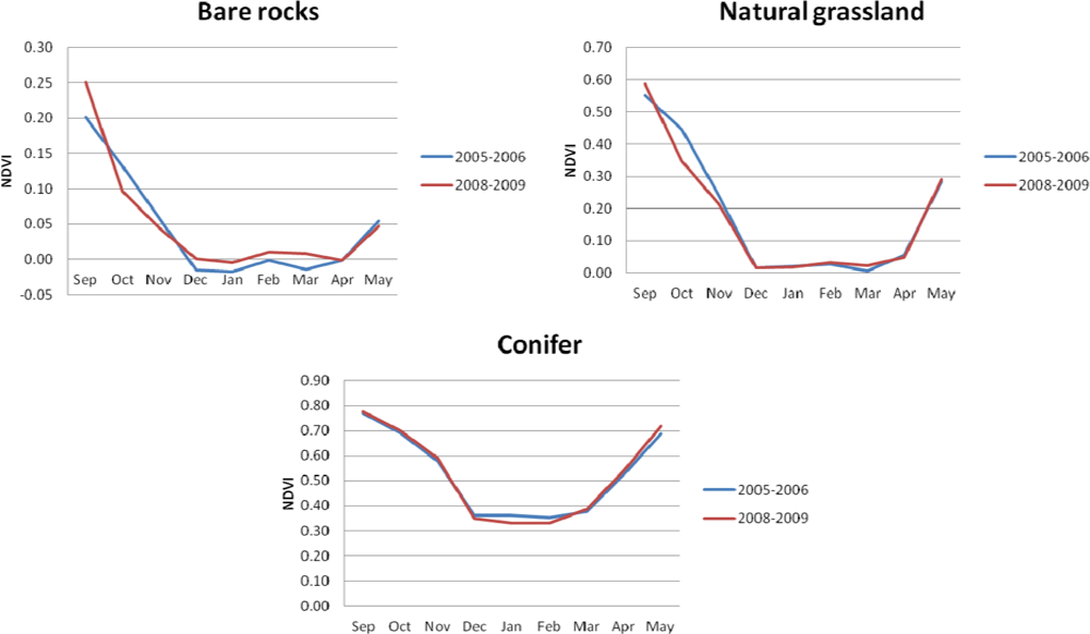
3.3. Snow Detection in Forest Module

For the detection of snow in forested areas, a multi-temporal approach is used, exploiting for B1 the ratio between the image to be classified and a snow-free reference image. As a reference image, an average of ten eight-day composite images is considered to have stable reference and to avoid the daily fluctuations of the reflectance.
Pixels with ratio values above a certain threshold, which is different for the different forest types, are classified as snow covered. For mapping purposes the forest standings are divided in pure coniferous standings (evergreen), pure broad-leaved standings (deciduous) and mixed forest, as each class can interact with snow differently, based on its own proper characteristics.

Conifer:

Soon after a snowfall, snow may lie on the tree crown or branches for a short time. If B1 reflectance values are very high, in case of dense forest stands (NDVI values over a certain threshold), the presence of snow on the conifer trees can also be detected. Afterwards, the snow falls below the tree crown due to wind action, the snow weight itself, and can also disappear due to melting.
Therefore the radiometric contribution of the snow under the trees is partially masked by the tree canopy. The pure coniferous standings cover the snow beneath and hinder its detection with the optical sensors. In this case, the NDVI value and the ratio between the actual image (snow) and the reference image are considered. The approach is adapted after Klein et al.[29], but exploits only the NDVI variation in the multi-temporal comparison.
Three thresholds are defined for the following values:
  • - NDVI is lower for forest in winter with respect to summer with values around 0.2–0.4 [25] (Figure 4);
  • - B1 reflectance tc (topographically correct) values higher than 0.10–0.15 indicates the presence of snow due to the high value of snow reflectance even if mixed with forest reflectance;
  • - B1/B1ref indicates a difference with respect to the summer image in order to avoid misclassification in the evaluation of B1 reflectance due to problem of mixed pixels and the contribution of tree reflectance. Ratio values higher than 1.2–1.4 may indicate the presence of snow.

Broadleaf:

In the case of broadleaf forest, the presence of snow is less influenced by the presence of trees as the leaves are lost in fall. In the forest stands, a further subdivision is considered between dense and sparse forest to take into account the different tree density. This discrimination is performed based on NDVI thresholds, generally for values lower than 0.2. We have validated this discrimination in some selected areas by using Land Cover Classification Maps. Subsequently, the distinction of snow covered and snow-free areas is performed using the threshold on B1 band (for values higher than 0.10–0.25 based on the forest density).

Mixed:

in case of mixed forest, a threshold on B1 reflectance is considered. The mixed forest is quite complicated to be detected and the evaluation of the algorithm outputs is also very difficult. For this reason, only the threshold on B1 reflectance is considered (for values higher than 0.10–0.15).

3.4. Cloud Module

The cloud module is divided in two steps. The first step is performed on band 4 and 6 of MOD09GA and MYD09GA images (500 m), thus exploiting the different absorption of cloud and snow in these bands. It is the same principle on which the NDSI works. The comparison with several snow covered areas in different illumination conditions suggested that the threshold on the mean values of these bands (B6 + B4)/2 is more suitable to detect the snow. With respect to values found in literature, some adaptations need to be carried out. For example, in alpine areas, it was found that B6 > 0.2 is suitable since it has been proved that the reflectance of many clouds, particularly over the snow covered areas, have values between 0.2 and 0.3 [14].
This threshold works well to discriminate snow from most of the obscuring clouds, because clouds show a high reflectance in the visible and near-infrared part of the electromagnetic spectrum including part of the mid-infrared [30], whereas the reflectance of the snow drops strongly in thermal infrared part of the spectrum due to absorption.
This threshold, however, is not enough to identify or discriminate thin cirrus clouds which behave in this part of the spectrum similarly to snow. In this case, a second part of the module introduces the use of the brightness temperature at 11 μm, thus allowing discrimination of this type of cloud.
This step of the cloud cover detection uses MOD021KM or MYD021KM (1 km) product as indicated in Ackerman et al.[31]. In the context of the alpine environment, the thresholds are adjusted to fit the local conditions. The threshold retrieval is obtained on a statistical basis.
The applied procedure performs an orthorectification and geocoding of MODIS021KM-level 1B (Reflectance and emissive bands) of the following bands: 20, 21, 31, 32, 26.
The emissive bands have to be converted in brightness temperatures (BT), while band 26 can be entered directly in the calculation of the thresholds.
In order to detect the cloud cover the following tests are performed: test1, BT 11; test2, BT 11–BT 3.7; test3, BT 3.7–BT 3.9; test4, 1.38 (band 26); test5, BT 3.7–BT 12.
Different tests are related to different cloud types. In particular, the difference BT 3.7–BT 12 provides an improved estimation of the cloud mask [3].
The probability of a pixel being cloud free or cloud covered is determined on the different test by using the approach of Ackerman et al.[31], but adapted to meet the conditions of the areas under investigation. The different test outputs are then averaged and the resulting final map has values between 0 (completely cloud covered sky) and 1 (completely cloud free sky). Intermediate values are classified on the basis of previous statistical analysis. Based on work of Ackerman et al.[31], for values between 0 and 0.66, pixels have a probability higher than 95% of being cloudy. For more details on the cloud module, the authors can refer the literature [31,32].

3.5. Merging Aqua and Terra SCA Maps

An improved snow cover product can be obtained by combination of snow maps derived from MODIS Terra and Aqua sensors [3336]. In fact, their different acquisition mode and time (morning acquisitions for Terra in descending mode and late morning and/or afternoon acquisitions for Aqua in ascending mode) determine a reduction in both cloud coverage and pixels without valuable information due to the different illumination conditions and satellite viewing angle.

3.6. Product Delivery Information

As mentioned earlier, the SCA maps can be processed by using MODIS images received directly from the EURAC receiving station. After the pre-processing of the Levil1b and Level2 MODIS Products, that can take up to 2 h, the EURAC snow module is capable of producing snow maps in a few minutes. Therefore, starting from the image acquisitions, the maps are delivered to the users in a few hours. An example is presented in Table 1. The SCA maps are released in GEOTIFF format and with ETRS89/ETRS-LAEA reference system.
Two kinds of products can be delivered:
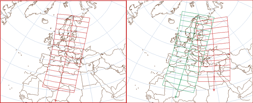
  • - single SCA map (indicated as IM) based on MODIS Terra or Aqua images on the area where the acquisitions are available;
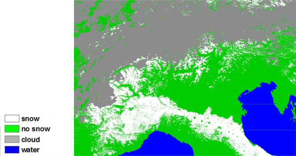
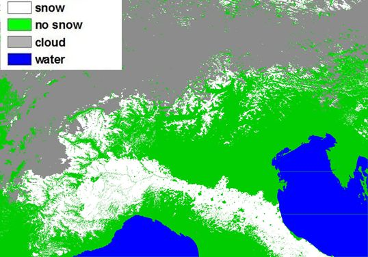
  • - enhanced SCA maps (indicated as CM) based on a combination of snow maps derived from MODIS Terra and Aqua acquisitions on the area where the acquisitions are available, thus reducing both cloud and “no data”-pixel. To obtain a complete coverage of the area of interest, a single pass is sometimes enough, while in other cases, two consecutive passes from the same satellite are required. Examples of these two cases are respectively shown in Figure 5 for the Terra satellite.

4. SCA Maps Quality Indices

The final SCA maps have also some other auxiliary files indicating the technical quality (successful acquisitions and any other technical issues) and the scientific quality maps. The file contains five layers, of which the first layer is the snow map. For all quality flags the following levels of accuracy are identified:
  • 0: missing data;
  • 1: low quality;
  • 2: medium quality;
  • 3: high quality.
The quality layer for snow is based on the NDSI.
The SCA maps obtained with the proposed approach are compared to the output of the standard snow index map (NDSI, based on 500 m resolution), obtaining the following cases:
  • - In the case that both the standard NDSI indicates a high snow probability (NDSI > 0.7) and the proposed SCA have also detected snow, the data are flagged as high quality.
  • - In the case that the NDSI maps indicate a medium snow probability (0.4 < NDSI < 0.7) and the proposed SCA maps detect snow, the data are flagged as medium quality.
  • - In the case that the NDSI values indicate low probability of snow (NDSI < 0.4) and the proposed SCA maps detect snow, these pixels are flagged as low quality.
For cloud detection, the following cases are categorized based on the cloud probability value described in Section 3.4:
  • - Cloudy pixels set to “HIGH” have a probability value in the cloud mask higher than 95%.
  • - Cloudy pixels set to “MEDIUM” have a probability value in the cloud mask between 95% and 68%.
  • - Cloudy pixels set to “LOW” have a probability value in the cloud mask lower than 68%.
The quality based on input reflectance data is used to detect missing or uncorrected reflectances values in the input data. The NASA corrected reflectance input data can have negative values. This can appear over very dark surfaces as, e.g., an ocean or under complete shadow of the mountains. As these negative values are not scientifically useful for snow detection, these values are flagged as low quality.
The last layer is based on satellite viewing geometry. This quality flag is related to the fact that data have a lower quality for certain viewing conditions (depending on the satellite and sensor relative position) and these data are flagged accordingly:
  • - High quality when the solar zenith is less than 85.0° and sensor zenith is less than 60°;
  • - medium quality when the solar zenith is either greater than 85.0° or sensor zenith is greater than 60°;
  • - low quality when the solar zenith is greater than 85.0° and sensor zenith is greater than 60°.
This follows the NASA rules, used for the merging of the NASA MOD09 data (MOD09 user’s guide, http://dratmos.geog.umd.edu/products/MOD09_UserGuide_v1_3.pdf).
The layers are provided separately as independent information to the SCA maps and are not used in the SCA algorithm.

5. Results

Figure 6 illustrates an example over the area of Central Europe acquired on 18 April 2011, while Figure 7 reports an example of SCA maps during winter 2011–2012. More detail in Figure 7 illustrates the snow cover areas during the snowfall for Po valley areas at the beginning of February 2012. Figure 8 illustrates some details of the EURAC snow cover maps with respect to MODIS standard algorithm and RGB images. The areas were selected in mountain regions to better highlight the usefulness of 250 m snow cover in such areas. The comparison with RGB indicates how the 250 m SCA maps are able to detect features that in the 500 m SCA maps are missed due to the resolution. This aspect is quite important when dealing with snow cover detection in small watersheds and in relation to data assimilation in high resolution hydrological models.
The maps in Figures 6 and 7 are combined maps derived from Terra and Aqua acquisitions acquired on the same day. Preliminary results indicate that in average in some cases, the decrease of the cloud cover can be around 20–25% [35]. Also, Parajka and Blöschl [34] found a decrease in snow cover over Austria of up to 21% depending on the season. In Figure 6, the cloud reduction was around 8%.
An analysis carried out by Thirrel et al.[37] on the SCA maps generated with the proposed algorithm and with corresponding MODIS SCA standard products indicates that over one year (365 days):
  • - The proposed algorithm determines from 200 to 310 available SCA maps;
  • - MODIS algorithm produces from 150 to 280 available SCA maps.
This effect is due to the more conservative algorithm for cloud detection with respect to NASA SCA products which make a strict selection over the analyzed areas.
Further and more detailed analyses are presented in the companion paper [23].

6. Conclusions

A new algorithm for snow detection from MODIS images at 250 m is proposed. The main advantage of the proposed approach lies in the exclusive use of 250 m for the snow maps. This allows better highlighting of the snow variability, especially in complex terrain such as mountainous areas.
The algorithm is composed of different modules, each tailored to meet the regional conditions over Europe and, in particular, of mountainous areas.
The main concept behind the proposed approach is twofold. First, the use of 250 m bands allows for the obtaining of more detailed maps. Second, the snow algorithm and the cloud detection have been developed through trying to meet local conditions. One advantage with respect to detection of snow cover fraction is that the snow detection is carried out at pixel level with a simple decision tree approach, thus reducing the impact of the snow detection in the pixel of 500 m, using as a reference high resolution images (Landsat) and/or unmixing approaches.
The SCA maps are further qualified by the addition of four quality layers for snow detection, cloud detection, input reflectances and viewing geometry. These quality flags identify problematic areas and permit the proper evaluation of the final SCA maps.
The SCA maps are delivered to users in near real-time, around 4 h after MODIS image acquisitions and downloading, thanks to the availability of a receiving station.
The proposed algorithm has been extensively validated by comparison with high resolution SCA maps derived from Landsat 7 ETM+ images and with snow depth measured from ground stations in selected test sites in Austria, Slovakia, Germany and Italy, as detailed in the companion paper [23].
Moreover, a comparison with the NASA standard SCA products MOD10 (MYD10) was carried out. The comparison with Landsat and MOD11 (MYD11), carried out on the same overlapped area, revealed similar trends. In particular, when the algorithm is exclusively based on NDVI to maintain the 250 m resolution, the snow detection in forest areas suffers. In a detailed comparison with Landsat and MODIS, the snow maps indicate an accuracy range between 88.1%–93.6% and 85.4%–95.3%, respectively. The lower accuracy values are related to forested areas when in open free areas the performances are quite similar, with the advantage of detecting more detailed features with respect to the 500 m MOD10 (MYD10) maps.
Moreover, an analysis carried out by Thirrel et al.[37] indicates that the improved and locally adapted cloud cover maps increase the availability of snow maps by approximately 20%. The comparison with ground snow depth measurements indicates a variability in the accuracy between 82% and 94%, where the lowest values of accuracy are found in steepest terrain.
The main drivers for the development of a 250 snow algorithm were both the necessity to have a higher resolution map to better detect snow variability in mountainous terrain with high variable topography and also to deliver the map in real-time. These requests come from local users and from research proposals. Actually, the maps are provided on a daily basis to South Tyrol Civil Protection and they are used in their own early warning system to provide information on avalanche risk, as well as for touristic activities. An experimental test in collaboration with the EU Joint Research Centre in Ispra (Italy) has also been carried out in order to check the feasibility of a real-time delivery for ingestion in a hydrological model for flood forecast, LISFLOOD [37].

References

  1. Roy, A.; Royer, A.; Turcotte, R. Improvement of springtime stream-flow simulations in a boreal environment by incorporating snow-covered area derived from remote sensing data. J. Hydrol 2010, 390, 35–44. [Google Scholar]
  2. Dozier, J.; Painter, T.H. Multispectral and hyperspectral remote sensing of alpine snow properties. Ann. Rev. Earth Planet. Sci 2004, 32, 465–494. [Google Scholar]
  3. Hall, D.K.; Riggs, G.; Salomonson, V.V.; DiGirolamo, N.E.; Bayr, K.J. MODIS snow-cover products. Remote Sens. Environ 2002, 83, 181–194. [Google Scholar]
  4. Clark, M.P.; Slater, A.G.; Barrett, A.P.; Hay, L.E.; McCabe, G.J.; Rajagopalan, B.; Leavesley, G.H. Assimilation of snow covered area information into hydrologic and land-surface models. Adv. Water Resour 2006, 29, 1209–1221. [Google Scholar]
  5. Tekeli, A.E.; Akyürek, Z.; Şorman, A.A.; Şensoy, A.; Şorman, A.Ü. Using MODIS snow cover maps in modeling snowmelt runoff process in the eastern part of Turkey. Remote Sens. Environ 2005, 97, 216–230. [Google Scholar]
  6. Dietz, A.J.; Wohner, C.; Kuenzer, C. European snow cover characteristics between 2000 and 2011 derived from improved MODIS daily snow cover products. Remote Sens 2012, 4, 2432–2454. [Google Scholar]
  7. Wang, X.; Xie, H.; Liang, T. Evaluation of MODIS snow cover and cloud mask and its application in Northern Xinjiang, China. Remote Sens. Environ 2008, 112, 1497–1513. [Google Scholar]
  8. Hall, D.K.; Riggs, G.A. Accuracy assessment of the MODIS snow-cover products. Hydrol. Process 2007, 21, 1534–1547. [Google Scholar]
  9. Klein, A.G.; Barnett, A. Validation of daily MODIS snow maps of the Upper Rio Grande River Basin for the 2000–2001 snow year. Remote Sens. Environ 2003, 86, 162–176. [Google Scholar]
  10. Liang, T.G.; Huang, X.D.; Wu, C.X.; Liu, X.Y.; Li, W.L.; Guo, Z.G. An application of MODIS data to snow cover monitoring in a pastoral area: A case study in Northern Xinjiang, China. Remote Sens. Environ 2008, 112, 514–1526. [Google Scholar]
  11. Maurer, E.P.; Rhoads, J.D.; Dubayah, R.O.; Lettenmaier, D.P. Evaluation of the snow covered area data product from MODIS. Hydrol. Process 2003, 17, 59–71. [Google Scholar]
  12. Zhou, X.; Xie, H.; Hendrickx, M.H.J. Statistical evaluation of remotely sensed snow-cover products with constraints from streamflow and SNOTEL measurements. Remote Sens. Environ 2005, 94, 214–231. [Google Scholar]
  13. Metsämäki, S.; Vepsäläinen, J.; Pulliainen, J.; Sucksdorff, Y. Improved linear interpolation method for the estimation of snow-covered area from optical data. Remote Sens. Environ 2002, 82, 64–78. [Google Scholar]
  14. Malcher, P.; Floricioiu, D.; Rott, H. Snow Mapping in Alpine Areas Using Medium Resolution Spectrometric Sensors. Proceedings of IEEE International Geoscience and Remote Sensing Symposium, Toulouse, France, 21–25 July 2003; 4, pp. 2835–2837.
  15. Warren, S.G. Optical properties of snow. Rev. Geophys. Space Phys 1982, 20, 67–89. [Google Scholar]
  16. Sirguey, P.; Mathieu, R.; Arnaud, Y. Subpixel monitoring of the seasonal snow cover with MODIS at 250 m spatial resolution in the Southern Alps of New Zealand: Methodology and accuracy assessment. Remote Sens. Environ 2009, 113, 160–181. [Google Scholar]
  17. Salomonson, V.V.; Appel, I. Development of the Aqua MODIS NDSI fractional snow cover algorithm and validation results. IEEE Trans. Geosci. Remote Sens 2006, 44, 1747–1756. [Google Scholar]
  18. Parajka, J.; Blöschl, G. MODIS-Based Snow Cover Products, Validation, and Hydrologic Applications. In Multiscale Hydrologic Remote Sensing Perspectives and Applications; Chang, N.-B., Hong, Y., Eds.; CRC Press: Boca Raton, FL, USA, 2012; pp. 185–212. [Google Scholar]
  19. Vikhamar, D.; Solberg, R. Snow-cover mapping in forests by constrained linear spectral unmixing of MODIS data. Remote Sens. Environ 2003, 88, 309–323. [Google Scholar]
  20. Painter, T.H.; Rittger, K.; McKenzie, C.; Slaughter, P.; Davis, R.E.; Dozier, J. Retrieval of subpixel snow covered area, grain size and albedo from MODIS. Remote Sens. Environ 2009, 113, 868–879. [Google Scholar]
  21. Rittger, K.; Painter, T.H.; Dozier, J. Assessment of methods for mapping snow cover from MODIS. Adv. Water Resour. 2012; in press. [Google Scholar]
  22. GCOS. Systematic Observation Requirements for Satellite-Based Data Products for Climate 2011 Update: Supplemental Details to the Satellite-Based Component of the “Implementation Plan for the Global Observing System for Climate in Support of the UNFCCC (2010 Update); WMO: Geneva, Switzerland, 2011; Available online: http://www.wmo.int/pages/prog/gcos/Publications/gcos-154.pdf (accessed on 15 December 2012).
  23. Notarnicola, C.; Duguay, M.; Moelg, N.; Schellenberger, T.; Tetzlaff, A.; Monsorno, R.; Costa, A.; Steurer, C.; Zebisch, M. Snow cover maps from MODIS images at 250m resolution, Part 2: validation. Remote Sens 2012. submitted.. [Google Scholar]
  24. MODIS Surface Reflectance User’s Guide, Version 1.3;; February 2011. Available online: http://modis-sr.ltdri.org/ (accessed on 15 December 2012).
  25. Civco, D.L. Topographic normalization of Landsat Thematic Mapper digital imagery. Photogramm. Eng. Remote Sensing 1980, 46, 1191–1200. [Google Scholar]
  26. Crane, R.G.; Anderson, M.R. Satellite discrimination of snow/cloud surfaces. Int. J. Remote Sens 1984, 5, 213–223. [Google Scholar]
  27. Dozier, J. Spectral signature of alpine snow cover from the Landsat thematic mapper. Remote Sens. Environ 1989, 28, 9–22. [Google Scholar]
  28. Lopez, P.; Sirguey, P.; Arnaud, Y.; Pouyaud, B.; Chevallier, P. Snow cover monitoring in the Northern Patagonia ice field using MODIS satellite images (2000–2006). Glob. Planet Change 2008, 61, 103–116. [Google Scholar]
  29. Klein, A.G.; Hall, D.K.; Riggs, G.A. Improving snow-cover mapping in forests through the use of a canopy reflectance model. Hydrol. Process 1998, 12, 1723–1744. [Google Scholar]
  30. Russow, W.B.; Garder, L.C. Validation of ISCCP cloud detection. J. Climate 1993, 6, 2370–2393. [Google Scholar]
  31. Ackerman, S.; Strabala, K.; Menzel, P.; Frey, R.; Moeller, C.; Gumley, L.; Baum, B.; Seemann, S.W.; Zhang, H. Discriminating Clear-Sky from Cloud with MODIS Algorithm Theoretical Basis Document (MOD35), MODIS Cloud Mask Team Version 5.0. October 2006.
  32. Cappelluti, G.; Morea, A.; Notarnicola, C.; Posa, F. Automatic detection of local cloud systems from MODIS data. J. Appl. Meteorol. Climatol 2006, 45, 1056–1072. [Google Scholar]
  33. Gafurov, A.; Bárdossy, A. Cloud removal methodology from MODIS snow cover product. Hydrol. Earth Syst. Sci 2009, 13, 1361–1373. [Google Scholar]
  34. Parajka, J.; Blöschl, G. Spatio-temporal combination of MODIS images—Potential for snow cover mapping. Water Resour. Res 2008, 44, W03406. [Google Scholar]
  35. Rastner, P.; Irsara, L.; Schellenberger, T.; Della Chiesa, S.; Bertoldi, G.; Endrizzi, S.; Notarnicola, C.; Steurer, C.; Zebisch, M. Snow Cover Monitoring and Modelling in the Alps Using Multi Temporal MODIS Data. Proceedings of the International Snow Science Workshop, Davos, Switzerland, 27 September–2 October 2009.
  36. Wang, X.; Xie, H. New methods for studying the spatiotemporal variation of snowcover based on combination products of MODIS Terra and Aqua. J. Hydrol 2009, 371, 192–200. [Google Scholar]
  37. Thirrel, G.; Notarnicola, C.; Kalas, M.; Zebisch, M.; Schellenberger, T.; Tetzlaff, A.; Duguay, M.; Mölg, N.; Burek, P.; de Roo, A. Assessing the quality of a real-time snow cover area product for hydrological applications. Remote Sens. Environ 2012, 127, 271–287. [Google Scholar]
Figure 1. Area covered by the EURAC receiving station (red circle) and area covered by the snow product presented in this paper (yellow rectangle).
Remotesensing 05 00110f1
Figure 2. Overview of the processing steps for SCA map generation.
Remotesensing 05 00110f2
Figure 3. Overview of the processing steps of the three main modules dedicated respectively to snow, snow in forest and cloud detection.
Remotesensing 05 00110f3
Figure 4. NDVI variability expressed in monthly averages from September to May in bare rocks, natural grassland and conifer classes.
Remotesensing 05 00110f4
Figure 5. MODIS Terra coverage in single pass (left) and two passes (right).
Remotesensing 05 00110f5
Figure 6. Example of SCA maps from MODIS (Terra and Aqua combined) data acquired over Europe on 18 April 2011 obtained with the EURAC algorithm.
Remotesensing 05 00110f6
Figure 7. Example of SCA maps from MODIS (Terra and Aqua combined) data acquired over Northern Italy on 16 February 2012 obtained with the EURAC algorithm. In this SCA, the intense snowfall of the Po valley is clearly detected.
Remotesensing 05 00110f7
Figure 8. Detailed examples of EURAC SCA maps in comparison to MOD10 images from NASA algorithm and RGB images.
Remotesensing 05 00110f8
Table 1. Acquisition and delivery time for EURAC SCA products (IM and CM) respectively for the day 28 February 2011. On this day, two Terra and one Aqua overpasses were acquired by EURAC receiving station.
SatelliteStart TimeIM Delivery TimeIM Elapsed TimeCM Delivery TimeCM Elapsed Time
Terra09:1911:0101:41
Terra10:5712:5802:0113:0702:10
Aqua12:4114:4802:0714:5802:17

