Post-Fire Canopy Height Recovery in Canada’s Boreal Forests Using Airborne Laser Scanner (ALS)

Canadian Forest Service, Natural Resources Canada, 506 West Burnside Road, Victoria, BC V8Z 1M5, Canada
*
Author to whom correspondence should be addressed.
Remote Sens. 2012, 4(6), 1600-1616; https://doi.org/10.3390/rs4061600
Submission received: 9 April 2012
/
Revised: 28 May 2012
/
Accepted: 29 May 2012
/
Published: 1 June 2012
Abstract
:Canopy height data collected with an airborne laser scanner (ALS) flown across unmanaged parts of Canada’s boreal forest in the summer of 2010 were used—as stand-alone data—to derive a least-squares polynomial (LSPOL) between presumed post-fire recovered canopy heights and duration (in years) since fire (YSF). Flight lines of the >25,000-km ALS survey intersected 163 historic fires with a known day of detection and fire perimeter. A sequential statistical testing procedure was developed to separate post-fire recovered canopy heights from pre-fire canopy heights. Of the 153 fires with >5 YSF, 121 cases (89%) could be resolved to a complete or partial post-fire canopy replacement. The estimated LSPOL can be used to estimate post-fire aboveground biomass and carbon sequestration in areas where alternative information is dated or absent. These LIDAR derived findings are especially useful as existing growth information is largely developed for higher productivity ecosystems and not applicable to these ecosystems subject to large wildfires.
1. Introduction
Forested areas in Canada’s northern regions are largely unmanaged and are not subject to resource surveys with the same level of detail or regularity as those in regions to the south [1–3]. Provincial survey activities are typically linked to strategic planning over managed forest areas where forest harvesting is practiced. Canada’s northern forested areas are generally low-productivity environments that are also distant from populations and markets. In the absence of harvesting, wildfire is the key agent of disturbance, and fire suppression is commonly not pursued. In an effort to augment monitoring and inventory activities in Canada’s northern forested regions, we carried out an airborne laser scanner (ALS) campaign during the summer of 2010. The objective was to obtain representative information about forest canopy height, model-based estimates of stem-volume, and biomass [4–6]. Using a discrete return scanning laser system, we flew 34 transects over a total distance of 25,000 km across Canada’s V boreal forests [7]. Based on the flying height and scan angle, the swath width of transects was 400 m or greater. Several transects (25) intersected areas burned in fires with a known incidence date and fire perimeter, with fires dating back to 1942. The most recent fire burned in 2007. The 2010 canopy heights derived from the ALS data provide a basis from which to estimate the rate of recovery of the vegetation after a fire [8–10]. Note that, due to remoteness and logistical considerations, the campaign did not include co-located collection of field data or other information in areas disturbed by fire.
Information on canopy recovery is important since canopy height is strongly correlated with live aboveground forest biomass, which, in turn, is correlated to the amount of carbon stored in aboveground live biomass components of a forested area [11–13]. Canopy height recovery following a forest fire is an important variable in the carbon balance of northern fire-driven forests [14,15]. We focus on years since fire rather than stand age, as there is a variable period of time during which regeneration initiates and local competition will regulate the return of trees to a given site [16,17].
The use of ALS data to estimate post-fire vertical vegetation recovery rates would be straightforward if forest fires consumed all live vegetation within a fire perimeter. In that case, the height of the vegetation immediately following the fire area would be zero, and the height of vegetation observed in 2010 would be the result of a post-fire recovery. Yet numerous studies have shown that most boreal forest fires leave a mosaic of surviving and dead standing vegetation elements within the outer perimeter of the area affected by a forest fire [18–23]. Areas registered as burned in the national Forest Fire Database [24] may include a mosaic of different starting points for the post-fire canopy recovery process.
A direct consequence of the potential of an incomplete fire consumption is that canopy heights estimated from the 2010 ALS data collected over formerly burned areas could be a mixture of heights from older surviving vegetation and younger post-fire regeneration [25–27]. With coincident and concurrent field data, or high spatial resolution satellite imagery, a separation could be supported using image-based change detection or interpretation [28,29]. This study demonstrates a procedure for the separation, when the only source of information comes from ALS data and publicly available archived Landsat images. Combined with estimates of canopy closure the results from this study will improve our estimates of carbon sequestration in areas where basic information about forest conditions and growth is limited in amount and distribution.
2. Material and Methods
2.1. ALS Data Acquisition
We acquired surface elevation data (latitude, longitude, elevation) in 34 individual survey flights between 14 June and 20 August 2010 with an Optech Airborne Laser terrain Mapper (ALTM) 3100 mounted in a twin engine PA31 Piper Navajo. The flight lines were situated between 56°W (Newfoundland) and 138°W (Yukon), and between latitudes 43°N and 65°N. Nominal acquisition parameters were: (a) a flying altitude of 1,200 m a.g.l.; (b) a velocity of 150 knots; (c) a pulse repetition frequency (PRF) of 70 kHz; and (d) a scan angle of ±15°. These parameters give a nominal multiple return density of ∼2.82 pts/m2, fully sufficient for the task at hand [30,31] The laser pulse footprint diameter in the standard narrow-beam divergence mode of 0.3 mRad is approximately 0.3 m at 1,200 m a.g.l. To reduce limitations to data collection, the acquisition plan we developed was flexible, allowing for flying around adverse weather, high relief, excessive fire and smoke activity, and restricted airspace, among other things. In so doing, we maximized flying and acquisition time by avoiding an overly prescribed flight plan that would have necessitated waiting out adverse conditions.
2.2. ALS Data Processing
We processed these strips of ALS data by integrating GPS and IMU (Inertial Measurement Unit) data with the laser range and scanner data to generate binary data files containing the laser point position, intensity, and scan angle information. We classified returns as first, intermediate, last, or single. Additional processing by the Applied Geomatics Research Group ( http://agrg.cogs.nscc.ca/, accessed 7 December 2011) created a ground return point dataset used to produce a 1-m DEM raster of ground elevation [32]. We overlaid the ALS “all-returns” point data onto this grid and subtracted the ground elevations to generate a canopy point data set. The accuracy of the DEM is expected to be around 0.3 m [33]. However, we acknowledge that in complex terrain or short-statured open scattered forests of the north with slow decaying woody-debris, hummocks of sphagnum, and dense shrubs, the accuracy can be lower (0.5–1.5 m) [34–36].
We then processed ALS data into a suite of plot-level canopy metrics, whereby returns from 2 m or more above the ground DEM elevation were classified to non-ground surface returns [37]. An ALS plot is a 25 × 25 m square, indexed to a 1:50,000-scale NTS sheet and located within 200 m from either side of a transect flight line. We consider these 25 × 25 m cells as LIDAR-plots, relating plot-like information for remote locations. We used the freely available FUSION software [38] to create a suite of distributional metrics for each LIDAR-plot. For this study we used the average canopy height, the standard deviation of canopy heights, and height-weighted mean canopy height (LHT): The first two were used to screen forested “plots” from non-forested plots. If the mean canopy height was greater than 2.0 m and the standard deviation above 1.0 m, we assumed the plot was a treed plot and we considered it for analysis. We considered values of LHT as proxies for Lorey’s height [39].
We also classified the land cover in each plot according to the classification system of the Earth Observation for Sustainable Development of forests (EOSD) project [40]. We restricted plots with pre-1990 fires to EOSD classes 200 and higher (“Forest/Trees”). As expected from knowledge of previous wildfire locations and trends [41,42], about 70% of the intersected burned areas were, in 2010, dominated by open or dense conifers.
2.3. Fire Data
We searched the national Large Fire (≥200 ha) Database [42] with geo-referenced centroid and perimeter (extent at time of extinction) of burned areas for intersections with the ALS flight lines. We found a total of 163 historic fires that intersect with the LIDAR transect flight lines. Of these intersected wildfires, nine were less than five years old at the time of over-flight in 2010 and were discarded because we cannot discriminate between shrubs and young trees at this early stage [43]. For each intersected fire, we had data on the years since fire (YSF), spatial data relating perimeter (fire boundary), and area (fire size). Fire sizes varied from 344 to 51,322 ha (mean = 2,778 ha), and the year of burning ranged from 1942 to 2007 with a median of 1990.
2.4. Estimating Post-Fire Tree Canopy Recovery
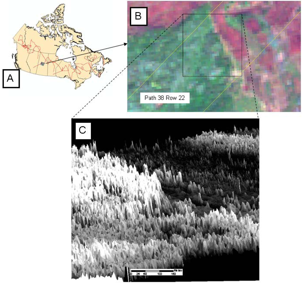
Without field data or high spatial resolution satellite imagery to support a partitioning of observed canopy heights to a pre-fire residual canopy or a post-fire regenerated canopy assumption, our starting point for the analysis was an assumption of approximately equal pre-fire canopy height distributions inside and outside of intersected fire perimeters. For large fires in the boreal forest, this is a reasonable working hypothesis since most unattended fires are extinguished by fire-stopping events, for example rain [44,45]. Fires also stop at natural boundaries (e.g., lakes, rivers, rock outcrops). With ALS-data and archived Landsat imagery we were able to identify and account for natural boundaries. “Outside” is defined here as the area covered by the LIDAR swath (200 m wide) and within a distance of 200 m from the fire perimeter. The 200 m width restriction is argued on the basis of the average spatial autocorrelation of 0.34 in mean height. In a 200 m long strip of 8 LIDAR plots, the average plot-to-plot correlation is approximately 0.05 and found significant at the 5% level. A wider buffer would yield a non-significant average correlation. A variogram-based analysis would result in a very similar choice of buffer width. We labeled LHT data from inside and outside a burned area as LHTin and LHTout respectively, and discarded data from a strip approximately 50 m wide centered on the fire boundary. Results with a discard within a 100 m separation belt were practically identical. Google Earth™ images from 2010–2011 were used as ancillary classification information and to improve interpretation of the LHT data ( http://www.google.com/earth/index.html, accessed 22 December 2011). A pictorial example illustrating the LIDAR transects, a Landsat TM image of a partially burned area, and a pseudo 3-D rendition of the corresponding LIDAR canopy heights are in Figure 1.
The task of apportioning a part or all of the LHTin observations to a post-fire canopy recovery was facilitated by first classifying the empirical distributions of LHTin and LHTout as either unimodal or multi-modal [46]. An important indicator for the classification of canopy heights to a pre-fire remnant canopy or a post-fire regenerated canopy was the apparent mean canopy height growth rate per year since the recorded fire, i.e., LH̄T × YSF−1. As a visual aide to our analyses, we also computed smoothed probability density functions of canopy heights f̂in,i(lht) and f̂out,i(lht), i= 1,…,154. A bi-weight kernel with a bandwidth of 1 m was used for this purpose [47].
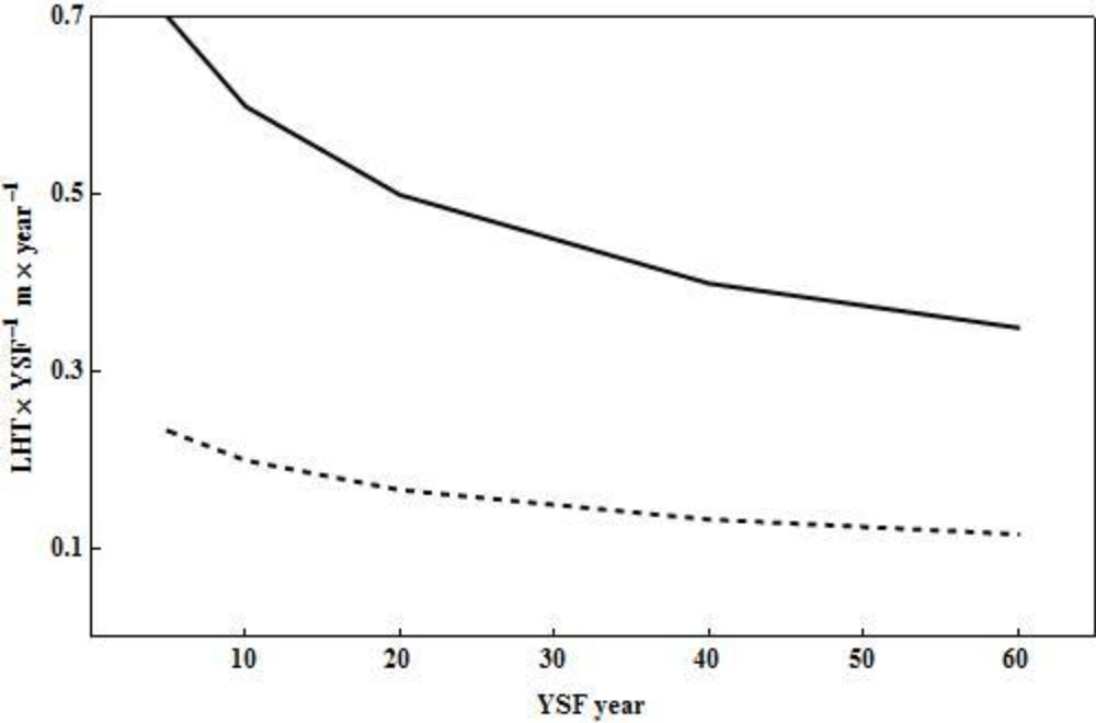
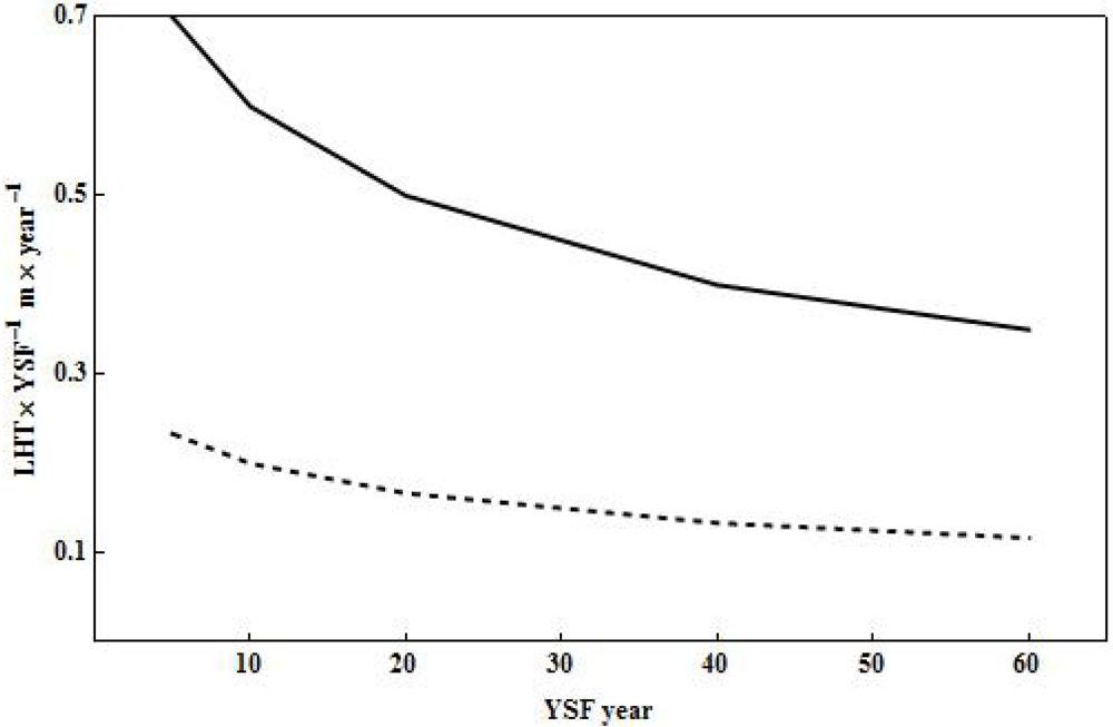
To determine whether a calculated height growth rate was commensurate with the hypothesis of a post-fire recovery, we established an upper bound for LH̄T×YSF−1. An apparent growth rate larger than this upper limit suggests that the current canopy predates the fire event. We determined the upper limit via a piecewise linear quantile regression [48] from a set of 1810 provincial, territorial, national and research (flux-tower) plots [3,49] located in the Boreal, the Taiga Shield, and the Taiga Cordillera ecozones ( http://sis.agr.gc.ca/cansis/nsdb/ecostrat/intro.html, accessed 22 December 2011). Since the plot(s) used to establish the upper limit were located further to the south, and since a majority of the plots were established in stand types with a commercial value, we assumed that the average height growth rate of intersected post-fire regeneration should fall below the 95th percentile regression line. The 95% confidence band for the plot-based estimates of height growth rates are in Figure 2. Thus, to be accepted as a post-fire regenerated canopy, the mean annual height growth LH̄T×YSF−1 should be less than LĤTQ95 × YSF−1. To accommodate the uncertainty in the quantile regressions (approximate standard error was 20 cm × year−1), we allowed an excess of up to 10%.
The stepwise screening of the 135 sets of twinned unimodal distributions of LHT and associated decision rules for deciding on the height of the post-fire recovered canopy is outlined in Table 1. The classification rules for the remaining 19 cases with a unimodal (inside and outside of a fire perimeter) distribution of LHT are in Table 2. Note, for the sake of brevity, only tests with a minimum of one positive outcome are listed.
All tests listed in Tables 1 and 2 were one-sided bootstrap t-tests [50] at the 5% level of significance and 600 replications. The sample size was, in all cases, min(50, nside / Sqrt[VIFside]), side = {in, out}, where VIF is the variance inflation factor [51] due to spatial autocorrelation in LHT (Pearson’s product moment correlation of LHT values in adjoining plots was 0.34). This choice of sample size ensured that differences in LHT larger than or equal to 1.2 m would be declared significant at the 5% level of significance at a rate of approximately 0.95 [52].
When LH̄Tin < LH̄Tout or when one or both of the distributions of LHT inside and outside the intercepted fire perimeter failed the test of a single mode at the 95% level of significance, we pooled LHTin and LHTout data and then separated it into two clusters via a k-means procedure [53]. A visual inspection of the LHT distributions data rarely suggested more than two clusters. We calculated cluster means and standard deviations for data from the inside and the outside of a fire perimeter and labeled them as LH̄Tside.clu, and ŝ(LHTside.clu) with clu = {1,2}, side = {in, out}. Decision rules for classifying clustered canopy heights are detailed in Tables 1 and 2.
As seen from Tables 1 and 2, in 32 cases we classified the observed distribution of LHTin to the pre-fire canopy category. An attempt to identify patches of post-fire regeneration by comparing Google Earth™ imagery to spatial k-means clusters of LHTin was unsuccessful (k ≤ 6). Since we could not repudiate that the left tail of f̂in,i(lht) contains elements of a post-fire recovering canopy, we assigned each case a default average annual post-fire canopy height growth rate equal to 0.5LĤTQ95 × YSF−1.
3. Results and Discussion
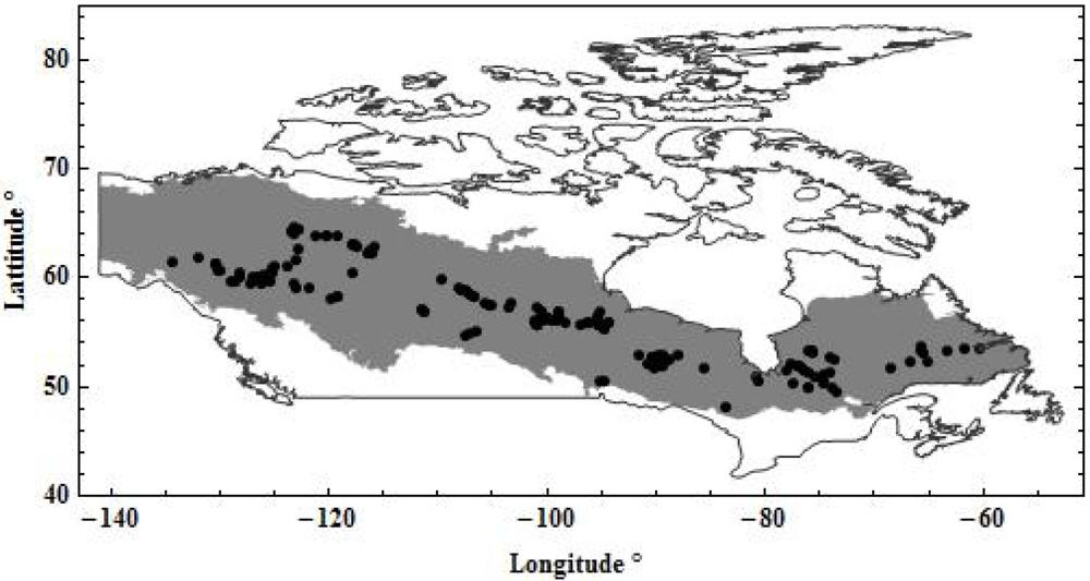
The spatial distribution of the 163 historic fires intersected by the ALS transects is shown in Figure 3. Fire perimeters were located between latitudes 48°10′ and 68°35′ and between longitudes −134°24′ and −60°22′. Overall, the sample of burned areas appears to be a small, yet fairly representative of the boreal forest.
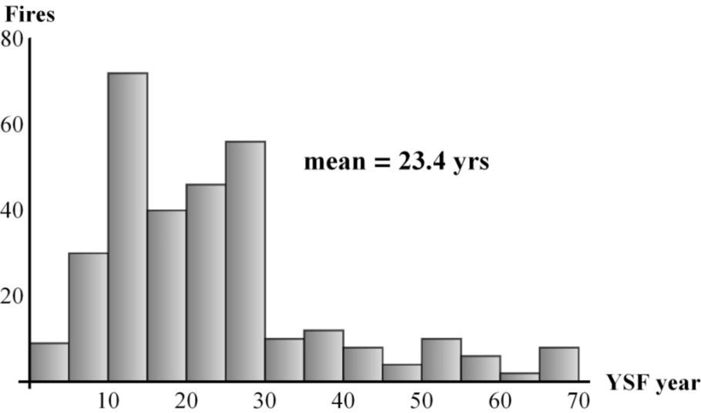
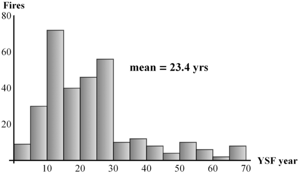
The years since fire (YSF) distribution in the study areas varied from 3 years to 68 years with a mean of 23 years (median 20 years) and a mode at 14 years (9%). Figure 4 illustrates the YSF distribution. Cases with an YSF-value of less than 5 years were not subject to analysis since the young age prevents us from discriminating between pre- and post-fire tree populations. Also, the distribution of YSF cannot be interpreted in terms of fire frequencies and fire cycles [54,55] due to incomplete records for fires prior to 1990 [42] generally coinciding with the advent of satellite remote sensing and the systematic, synoptic, mapping of large fires.
The classification of LHTin was facilitated by the large number of unimodal distributions. In 135 cases (88%) we accepted the null hypothesis of a unimodal distribution both inside and outside of the fire perimeter (diptest 5% level of significance [46]). Three randomly selected examples from the 34 (22%) cases where f̂in(LHT) was classified as the distribution of a post-fire regenerated canopy (Table 1, Step 1) are in Figure 5. Although the available data (YSF, f̂in(LHT), f̂out(LHT), LH̄TQ95, and satellite imagery) supported the classification, one cannot repudiate that both LH̄TQ95 and f̂out(LHT) may include heights from a pre-fire canopy.
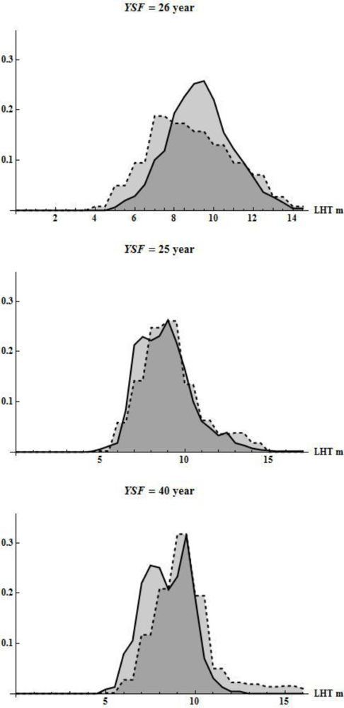
Three randomly selected examples from the largest group of 85 cases (56%) cases where f̂in(LHT) was classified as a mixed distribution of a pre- and post-fire canopy (Table 1, Step 2) are in Figure 6. In these cases f̂in(LHT) dominates f̂out(LHT) to the left of LH̄Tin. The assigned height to the post-fire canopy (LH̄Tin.1) is always smaller than the means of f̂in(LHT) and f̂out(LHT). The partitioning of f̂in(LHT) into a pre- and post-fire canopy distribution is, in the context of this study, a first approximation an attempt to fill an information gap in areas lacking basic forest inventory information. Clearly, field data, or high resolution imagery would have been preferred and improved the results [56].
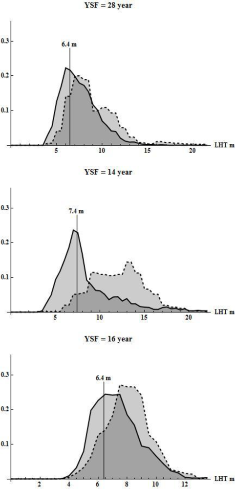
In 32 cases (21%) it was not possible to ascertain a post-fire regeneration of a tree canopy. Typically the fires were either too young (YSF < 10 years) to allow a clearly identifiable cohort of post-fire regeneration to emerge, or the apparent annual mean growth rate (LH̄Tin × YSF−1) of the observed canopy within a fire perimeter was greater than what can reasonably be expected (i.e., LH̄TQ95 × YSF−1). Three randomly selected cases from this group are shown in Figure 7. As indicated, the assigned default height to the post-fire canopy represents at most two percent of the observed height distribution inside the fire perimeter. Given a strong likelihood that the studied fires were caused by lightning and the low probability of surface fires in Canada’s north [22,33,46], we assumed that most of the observed height distribution emerged from a previous fire. Our database did not allow us to verify this assumption. In some cases the assigned “default” height may have been too high (recall, default computed as average annual post-fire canopy height growth rate equal to 0.5LĤTQ95 × YSF−1). It is known that boreal forest fires can create adverse conditions for post-fire regeneration, resulting in either a considerable delay in the recovery of a post-fire canopy or the growth of a vegetation type different from the one present prior to the fire [19,57,58]. A new LIDAR-based algorithm for separating forested from non-forested areas [59] may improve the discrimination of pre- and post-fire canopy height by eliminating areas that do not qualify as forest based on a minimum crown coverage definition.
Our results were not sensitive to the imposed minimum separation of 50 m between canopy heights from the inside and outside of the fire-perimeter. Analyses with a 100 m limit resulted in three additional rejections of unimodality and two fewer inconclusive cases. Estimates of canopy height recovery were practically identical with an adjusted coefficient of determination between the two set of estimates of 0.996 and the slope of 1.006 and intercept of −0.004 were statistically non-significant at the 0.05 level.
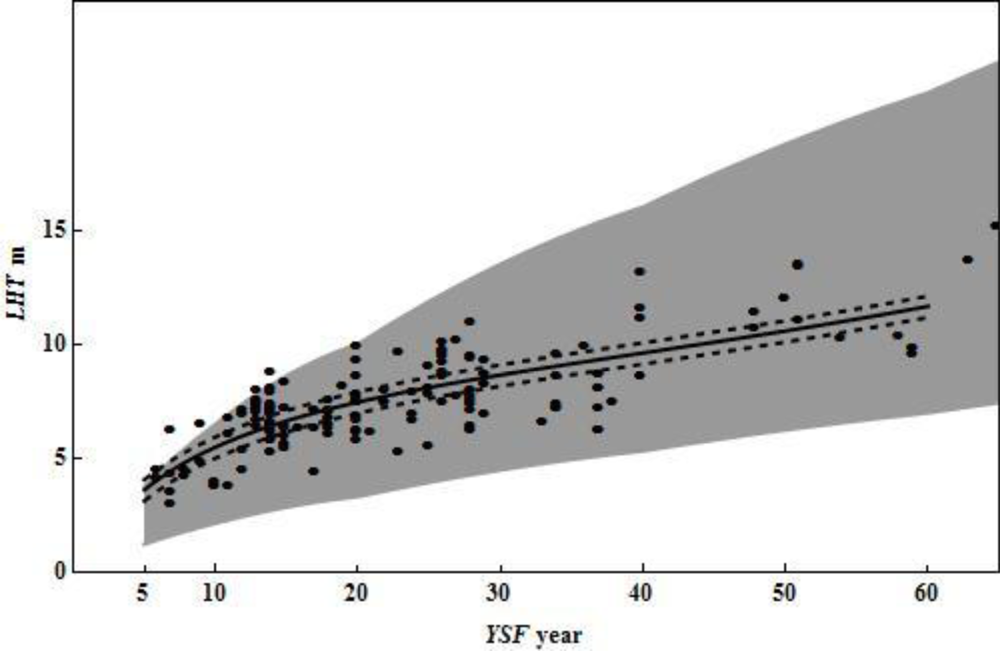
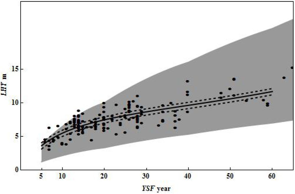
A summary of the 154 estimates of post-fire regenerated canopy heights is presented in Figure 8. A forward-stepwise regression analysis [60] with LH̄Tin × YSF−1 as the dependent variable and YSF, latitude (LAT), longitude, number of growing degree days, average daily maximum temperature (May-August) as explanatory variables identified YSF and LAT, as the only significant explanatory variables. Squared and square-root transformation of all explanatory variables were included in the stepwise screening which used a entry level of significance of 0.02, and a retention level of significance of 0.05 [61]. The model identified by the stepwise screening and re-transformed to a polynomial of LHTin in YSF is in Figure 8 (adjusted coefficient of determination = 0.63; residual standard error = 1.31 m).
The height–age model in Figure 8 can be converted to a model for the aboveground live biomass (AGBM) as a function of YSF and canopy closure and then to a model for sequestered carbon. The success of this approach requires validated biomass equations for post-fire regenerated stands [62]. The weak influence of location and two important climate variables was unexpected. Without an identification of species or a knowledge of the number of years it takes for stand establishment and regeneration after fire, we cannot determine if actual location effects have been masked by species differences and variation in the years it takes for trees to re-populate a burned area. Complex interactions between longitude and latitude is another potential masking issue. At a national scale, our sampling intensity is very low; an order of magnitude increase of additional locations would be necessary to determine geographic trends. Although the estimated standard error around the estimated YSF-trend in LHT is relatively large (1.3 m), the model is an important step forward towards an estimation of biomass and carbon sequestration, in areas of Canada’s boreal forest where we lack basic forest inventory information.
4. Conclusions
Post-fire tree canopy height distributions in boreal forests are typically composed of post-fire regeneration and pre-fire canopy elements. When canopy heights are derived from airborne laser scanner data an estimate of post-fire canopy recovery rates requires a separation of the burned and unburned structural elements. Without ancillary information, the separation must be based on statistical inference and generally accepted limits of tree height growth. In this study, we proposed and implemented a novel sequential statistical procedure for separating post- and pre-fire canopy elements. In so doing, we demonstrated that a separation of post- and pre-fire canopy elements could be identified and separated with confidence in most cases. Our approach serves to advance the capacity for understanding forest structural dynamics and regeneration rates following wildfire over remote boreal regions. A novel sequential statistical testing procedure was applied to stand-alone ALS data of canopy height collected over 163 previously burned areas in Canada’s boreal forest allowing us to separate pre- and post-fire canopies, and to estimate post-fire recovery rates with acceptable levels of precision. Inference based on Hartigan’s diptest was critical to the success of the study. Further improvements would be possible with the addition of high-resolution satellite imagery, although the limited image extents, relative to boreal wildfire areas, would result in unique challenges.
Acknowledgments
We thank Geordie Hobart of the Canadian Forest Service for data preparation and processing assistance. We thank The Canadian Interagency Forest Fire Centre and its member agencies ( http://www.ciffc.ca/) for developing the National Fire Database and for enabling our use of the data in this analysis.
References
- Leckie, D.G.; Gillis, M.D. Forest inventory in canada with emphasis on map production. For. Chron 1995, 71, 74–78. [Google Scholar]
- Wulder, M.A.; Kurz, W.A.; Gillis, M. National level forest monitoring and modeling in Canada. Progr. Plan 2003, 61, 365–381. [Google Scholar]
- Gillis, M.D.; Omule, A.Y.; Brierley, T. Monitoring canada’s forests: The national forest inventory. For. Chron 2005, 81, 214–221. [Google Scholar]
- Wulder, M.A.; Seemann, D. Forest inventory height update through the integration of LIDAR data with segmented landsat imagery. Can. J. Remote Sens 2003, 29, 536–543. [Google Scholar]
- Næsset, E. Accuracy of forest inventory using airborne laser scanning: Evaluating the first nordic full-scale operational project. Scand. J. For. Res 2004, 19, 554–557. [Google Scholar]
- Hudak, A.T.; Evans, J.S.; Smith, A.M.S. Lidar utility for natural resource managers. Remote Sens 2009, 1, 934–951. [Google Scholar]
- Brandt, J.P. The extent of the north american boreal zone. Env. Rev 2009, 17, 101–161. [Google Scholar]
- Angelo, J.J.; Duncan, B.W.; Weishampel, J.F. Using LIDAR-derived vegetation profiles to predict time since fire in an oak scrub landscape in east-central florida. Remote Sens 2010, 2, 514–525. [Google Scholar]
- Morsdorf, F.; Meier, E.; Kotz, B.; Itten, K.I.; Dobbertin, M.; Allgower, B. Lidar-based geometric reconstruction of boreal type forest stands at single tree level for forest and wildland fire management. Remote Sens. Environ 2004, 92, 353–362. [Google Scholar]
- Listopad, C.M.C.S.; Drake, J.B.; Masters, R.E.; Weishampel, J.F. Portable and airborne small footprint LIDAR: Forest canopy structure estimation of fire managed plots. Remote Sens 2011, 3, 1284–1307. [Google Scholar]
- Tinker, D.; Stakes, G.K.; Arcano, R.M. Allometric equation development, biomass, and aboveground productivity in ponderosa pine forests, black hills, wyoming. W. J. Appl. For 2010, 25, 112–119. [Google Scholar]
- Nabuurs, G.J. Special section: European forest carbon balance as assessed with inventory based methods. For. Ecol. Manage 2010, 260, 239–240. [Google Scholar]
- García, M.; Riaño, D.; Chuvieco, E.; Danson, F.M. Estimating biomass carbon stocks for a mediterranean forest in central spain using LIDAR height and intensity data. Remote Sens. Environ 2010, 114, 816–830. [Google Scholar]
- De Santis, A.; Chuvieco, E. Burn severity estimation from remotely sensed data: Performance of simulation versus empirical models. Remote Sens. Environ 2007, 108, 422–435. [Google Scholar]
- Bond-Lamberty, B.; Peckham, S.D.; Ahl, D.E.; Gower, S.T. Fire as the dominant driver of central canadian boreal forest carbon balance. Nature 2007, 450, 89–92. [Google Scholar]
- Gaboury, S.; Boucher, J.-F.; Villeneuve, C.; Lord, D.; Gagnon, R. Estimating the net carbon balance of boreal open woodland afforestation: A case-study in Québec’s closed-crown boreal forest. For. Ecol. Manage 2009, 257, 483–494. [Google Scholar]
- Lhermitte, S.; Verbesselt, J.; Verstraeten, W.W.; Veraverbeke, S.; Coppin, P. Assessing intra-annual vegetation regrowth after fire using the pixel based regeneration index. ISPRS J. Photogramm 2011, 66, 17–27. [Google Scholar] [Green Version]
- Escuin, S.; Navarro, R.; Fernández, P. Fire severity assessment by using NBR (normalized burn ratio) and NDVI (normalized difference vegetation index) derived from Landsat TM/ETM images. Int. J. Remote Sens 2008, 29, 1053–1073. [Google Scholar]
- Murphy, K.A.; Reynolds, J.H.; Koltun, J.M. Evaluating the ability of the differenced normalized burn ratio (DNBR) to predict ecologically significant burn severity in alaskan boreal forests. Int. J. Wildland Fire 2008, 17, 490–499. [Google Scholar]
- Cocke, A.E.; Fulé, P.Z.; Crouse, J.E. Comparison of burn severity assessments using differenced normalized burn ratio and ground data. Int. J. Wildland Fire 2005, 14, 189–198. [Google Scholar]
- Nappi, A.; Drapeau, P.; Saint-Germain, M.; Angers, V.A. Effect of fire severity on long-term occupancy of burned boreal conifer forests by saproxylic insects and wood-foraging birds. Int. J. Wildland Fire 2010, 19, 500–511. [Google Scholar]
- Hély, C.; Flannigan, M.; Bergeron, Y. Modeling tree mortality following wildfire in the southeastern canadian mixed-wood boreal forest. For. Sci 2003, 49, 566–576. [Google Scholar]
- Beverly, J.L.; Martell, D.L. Modeling pinus strobus mortality following prescribed fire in quetico provincial park, north-western Ontario. Can. J. For. Res 2003, 33, 740–751. [Google Scholar]
- Martell, D.L. Wildfire regime in the boreal forest. Conserv. Biol 2002, 16, 1177. [Google Scholar]
- Jaskierniak, D.; Lane, P.N.J.; Robinson, A.; Lucieer, A. Extracting LIDAR indices to characterise multilayered forest structure using mixture distribution functions. Remote Sens. Environ 2011, 115, 573–585. [Google Scholar]
- van Leeuwen, M.; Nieuwenhuis, M. Retrieval of forest structural parameters using LIDAR remote sensing. Eur. J. For. Res 2010, 129, 749–770. [Google Scholar]
- Kane, V.R.; Bakker, J.D.; McGaughey, R.J.; Lutz, J.A.; Gersonde, R.F.; Franklin, J.F. Examining conifer canopy structural complexity across forest ages and elevations with LIDAR data. Can. J. For. Res 2010, 40, 774–787. [Google Scholar]
- Dalponte, M.; Bruzzone, L.; Gianelle, D. Tree species classification in the southern alps based on the fusion of very high geometrical resolution multispectral/hyperspectral images and LIDAR data. Remote Sens. Environ 2012, 123, 258–270. [Google Scholar]
- Hudak, A.T.; Strand, E.K.; Vierling, L.A.; Byrne, J.C.; Eitel, J.U.H.; Martinuzzi, S.; Falkowski, M.J. Quantifying aboveground forest carbon pools and fluxes from repeat LIDAR surveys. Remote Sens. Environ 2012, 123, 25–40. [Google Scholar]
- Evans, J.; Hudak, A.; Faux, R.; Smith, A.M. Discrete return LIDAR in natural resources: Recommendations for project planning, data processing, and deliverables. Remote Sens 2009, 1, 776–794. [Google Scholar]
- Treitz, P.; Lim, K.; Woods, M.; Pitt, D.; Nesbitt, D.; Etheridge, D. Lidar sampling density for forest resource inventories in ontario, canada. Remote Sens 2012, 4, 830–848. [Google Scholar]
- Axelsson, P. DEM generation from laser scanner data using adaptive TIN models. Int. Arch. Photogramm. Remote Sens. Spat. Inf. Sci 2000, 33, Part B4/1. 110–117. [Google Scholar]
- Wulder, M.A.; White, J.C.; Bater, C.W.; Coops, N.C.; Hopkinson, C.; Gang, C. Lidar plots—A new large-area data collection option: Context, concepts, and case study. Can. J. Remote Sens 2012. submitted.. [Google Scholar]
- Tinkham, W.T.; Huang, H.; Smith, A.M.S.; Shrestha, R.; Falkowski, M.J.; Hudak, A.T.; Link, T.E.; Glenn, N.F.; Marks, D.G. A comparison of two open source LIDAR surface classification algorithms. Remote Sens 2011, 3, 638–649. [Google Scholar]
- Meng, X.; Currit, N.; Zhao, K. Ground filtering algorithms for airborne LIDAR data: A review of critical issues. Remote Sens 2010, 2, 833–860. [Google Scholar]
- Sharma, M.; Paige, G.B.; Miller, S.N. DEM development from ground-based LIDAR data: A method to remove non-surface objects. Remote Sens 2010, 2, 2629–2642. [Google Scholar]
- Bater, C.W.; Coops, N.C. Evaluating error associated with LIDAR-derived DEM interpolation. Comput. Geosci 2009, 35, 289–300. [Google Scholar]
- McGaughey, R.J. Fusion/LDV: Software for Lidar Data Analysis and Visualization; Pacific Northwest Research Station, Forest Service, USDA: Portland, OR, USA, 2010. [Google Scholar]
- Næsset, E. Practical large-scale forest stand inventory using a small-footprint airborne scanning laser. Scand. J. For. Res 2004, 19, 164–179. [Google Scholar]
- Wulder, M.A.; White, J.C.; Cranny, M.; Hall, R.J.; Luther, J.E.; Beaudoin, A.; Goodenough, D.G.; Dechka, J.A. Monitoring Canada’s forests. Part 1: Completion of the eosd land cover project. Can. J. Remote Sens 2008, 34, 549–562. [Google Scholar]
- Wotton, B.M.; Nock, C.A.; Flannigan, M.D. Forest fire occurrence and climate change in canada. Int. J. Wildland Fire 2010, 19, 253–271. [Google Scholar]
- Stocks, B.J.; Mason, J.A.; Todd, J.B.; Bosch, E.M.; Wotton, B.M.; Amiro, B.D.; Flannigan, M.D.; Hirsch, K.G.; Logan, K.A.; Martell, D.L.; et al. Large forest fires in canada, 1959–1997. J. Geophys. Res 2003, 108, 8149. [Google Scholar]
- Oswald, E.T.; Brown, B.N. Vegetation Establishment during 5 Years Following Wildfire in Northern British Columbia and Southern Yukon Territory; BC-X-320; Forestry Canada: Victoria BC, Canada, 1990; p. 46. [Google Scholar]
- Anderson, K. A model to predict lightning-caused fire occurrences. Int. J. Wildland Fire 2002, 11, 163–172. [Google Scholar]
- Girardin, M.P.; Wotton, B.M. Summer moisture and wildfire risks across canada. J. Appl. Meteor. Climatol 2009, 48, 517–533. [Google Scholar]
- Hartigan, J.A.; Hartigan, P.M. The dip test of unimodality. Ann. Stat 1985, 13, 70–84. [Google Scholar]
- Silverman, B.W. Density Estimation for Statistics and Data Analysis; Chapman & Hall: London, UK, 1986; p. 175. [Google Scholar]
- Koenker, R. Quantile regression for longitudinal data. J. Multivar. Anal 2004, 91, 74–89. [Google Scholar]
- Boudewyn, P.; Song, X.; Magnussen, S.; Gillis, M.D. Model-Based, Volume-to-Biomass Conversion for Forested and Vegetated Land in Canada; BC-X-411; Canadian Forest Service, Natural Resources Canada: Victoria, BC, Canada, 2007; pp. 1–111. [Google Scholar]
- Efron, B.; Tibshirani, R.J. An Introduction to the Bootstrap; Chapman & Hall: Boca Raton, FL, USA, 1993; p. 436. [Google Scholar]
- Engle, R.F. Autoregressive conditional heteroscedasticity with estimates of the variance inflation. Econometrica 1982, 50, 987–1007. [Google Scholar]
- Beal, S.L. Sample size determination for confidence intervals on the population mean and on the difference between two population means. Biometrics 1989, 45, 969–977. [Google Scholar]
- Hartigan, J.A. Clustering Algorithms; Wiley: New York, NY, USA, 1975; p. 351. [Google Scholar]
- Bergeron, Y.; Gauthier, S.; Kafka, V.; Lefort, P.; Lesieur, D. Natural fire frequency for the eastern canadian boreal forest: Consequences for sustainable forestry. Can. J. For. Res 2001, 31, 384–391. [Google Scholar]
- Reed, W.J.; Johnson, E.A. Statistical methods for estimating historical fire frequency from multiple fire-scar data. Can. J. For. Res 2004, 34, 2306–2313. [Google Scholar]
- Leckie, D.; Gougeon, F.; Hill, D.; Quinn, R.; Armstrong, L.; Shreenan, R. Combined high-density LIDAR and multispectral imagery for individual tree crown analysis. Can. J. Remote Sens 2003, 29, 633–649. [Google Scholar]
- Burton, P.J.; Parisien, M.; Hicke, J.A.; Hall, R.J.; Freeburn, J.T. Large fires as agents of ecological diversity in the north american boreal forest. Int. J. Wildland Fire 2008, 17, 754–767. [Google Scholar]
- Allen, J.L.; Sorbel, B. Assessing the differenced normalized burn ratio’s ability to map burn severity in the boreal forest and tundra ecosystems of Alaska’s national parks. Int. J. Wildland Fire 2008, 17, 463–475. [Google Scholar]
- Eysn, L.; Hollaus, M.; Schadauer, K.; Pfeifer, N. Forest delineation based on airborne LIDAR data. Remote Sens 2012, 4, 762–783. [Google Scholar]
- Draper, N.R.; Smith, H. Applied Regression Analysis; Wiley: New York, NY, USA, 1981; p. 709. [Google Scholar]
- Hocking, R.R. The analysis and selection of variables in linear regression. Biometrics 1976, 32, 1–49. [Google Scholar]
- Domke, G.M.; Woodall, C.W.; Smith, J.E.; Westfall, J.A.; McRoberts, R.E. Consequences of alternative tree-level biomass estimation procedures on u.S. Forest carbon stock estimates. For. Ecol. Manage 2012, 270, 108–116. [Google Scholar]
Figure 1.
Context and example of a LIDAR transect at the boundary of a burned area. A. Overview of entire 2010 LIDAR campaign over the Canadian Boreal forest denoted in red. B. Sub-scene from Landsat-5 Path 38 Row 22 October 2003 RGB image of bands (5,4,3) with generalized LIDAR transect outline in yellow and the 2002 wildfire scar identified by the pixels with shades of pink. C. Three dimensional surface view of a 0.5 m LIDAR Canopy Height Model with the wildfire impact illustrated, boundary evident and unburned islands also evident. The sub-scene is located in Saskatchewan and is centered at 54°50′30″N, 107°7′0″W.
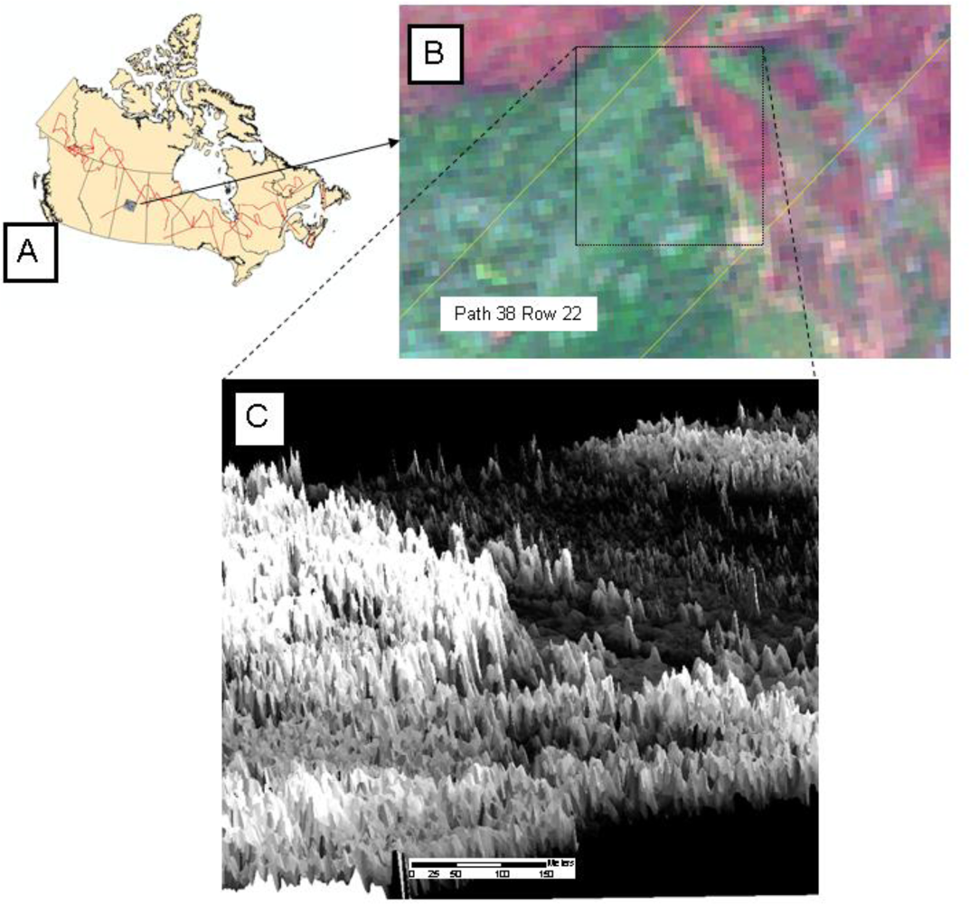
Figure 2.
Expected 95%-tile (full line) and 5%-tile (dashed) of average annual growth rate in mean canopy height (LHT m × year−1) in 1920 field plots in the Boreal, Taiga Shield, and Taiga Cordillera ecozones located to the south of the studied historic fires.
Figure 2.
Expected 95%-tile (full line) and 5%-tile (dashed) of average annual growth rate in mean canopy height (LHT m × year−1) in 1920 field plots in the Boreal, Taiga Shield, and Taiga Cordillera ecozones located to the south of the studied historic fires.

Figure 3.
Location map of centroids of intersected fire perimeters (black dots). The Canadian portion of the North-American boreal forest is gray-shaded [7].
Figure 3.
Location map of centroids of intersected fire perimeters (black dots). The Canadian portion of the North-American boreal forest is gray-shaded [7].
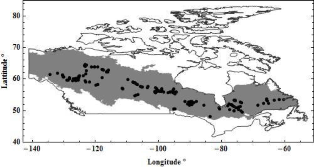
Figure 4.
Number of intersected fire perimeters by years since fire (YSF).

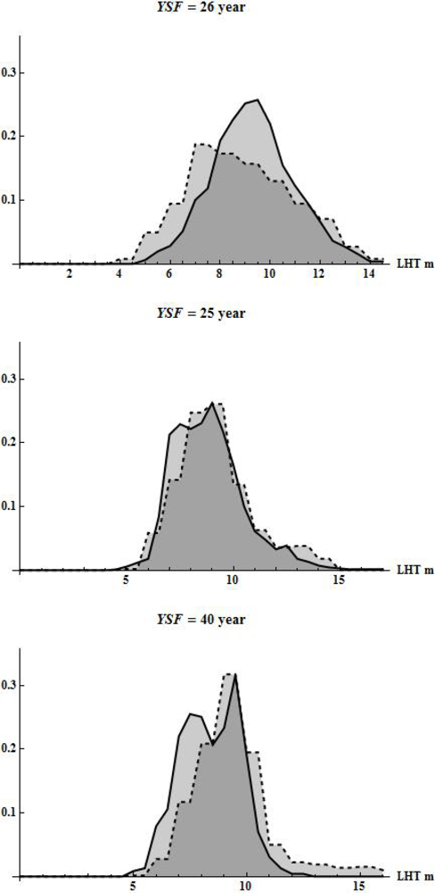
Figure 5.
Three randomly selected examples of probability distributions (34) of LHTin (full outline) classified as a post-fire canopy (Table 1, Step 1). The distribution of LHTout is indicated (dashed outline).
Figure 5.
Three randomly selected examples of probability distributions (34) of LHTin (full outline) classified as a post-fire canopy (Table 1, Step 1). The distribution of LHTout is indicated (dashed outline).

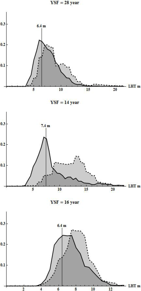
Figure 6.
Three randomly selected examples of distributions (85) of LHTin (full outline) classified as a partial post-fire canopy (Table 1, Step 2). The estimated mean height of the post-fire recovered canopy is indicated. The distribution of LHTout is indicated (dashed outline).
Figure 6.
Three randomly selected examples of distributions (85) of LHTin (full outline) classified as a partial post-fire canopy (Table 1, Step 2). The estimated mean height of the post-fire recovered canopy is indicated. The distribution of LHTout is indicated (dashed outline).

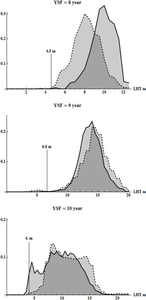
Figure 7.
Three randomly selected examples (of 32) without an identified post-fire recovered canopy. The assigned default canopy height is indicated. The distributions of LHTin (full outline) and LHTout (dashed outline) are indicated.
Figure 7.
Three randomly selected examples (of 32) without an identified post-fire recovered canopy. The assigned default canopy height is indicated. The distributions of LHTin (full outline) and LHTout (dashed outline) are indicated.
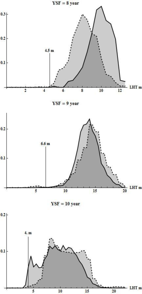
Figure 8.
Trends in mean post-fire regenerated canopy heights across years since fire (YSF). Trends are estimated for the median (full line) and maximum and minimum latitude (dashed) of the fire locations. The fitted regression model is:
.
= 0.78,
= 90.12 (P < 0.01). A 95% confidence interval for LHT determined from field plots located to the south of the studied fires is shaded in gray.

Table 1.
Classification of 135 (out of 153) unimodal distributions of LHTin to pre- and post-fire canopy heights when the empirical distribution of LHTout also passed the test of a single mode. See text for a definition of LH̄Tin.1.
| Step | Classification Rule (Test) | Classification of LHTin | Cases | Avg. Post-Fire Height Growth m × year−1 |
|---|---|---|---|---|
| 1 | YSF ≥ 25 and LH̄Tin ≤1.1LĤTQ95 and |LH̄Tin -LH̄Tout|< 1.2 m | Post-fire canopy | 34 | |
| 2 | LH̄Tin ≥ LH̄Tout + 1.2 m and LH̄Tin < 1.1LĤTQ95 | Partial post-fire canopy | 85 | |
| 3 | LH̄Tin ≥1.1LĤTQ95 | Pre-fire canopy | 16 |
Table 2.
Classification of 19 (out of 154) distributions of LHTin to pre- and post-fire canopy heights when either LHTin, or LHTout or both failed the diptest of a single mode.
| Step | Classification Rule (Test) | Classification of LHTin | Cases | Avg. Post-Fire Height Growth m × year−1 |
|---|---|---|---|---|
| Step 1 | LH̄Tin.1 ≤ LH̄Tout.1 and LH̄Tin.2 ≤ LH̄Tout.2 and LH̄Tin.1 ≤ LĤTQ95 and LH̄Tin.2 ≤ LĤTQ95 | Post-fire canopy | 1 | |
| Step 2 | LH̄Tin.1 ≤ LH̄Tout.1 and LH̄Tin.2 > LH̄Tout.2 LH̄Tin.1 ≤ LĤTQ95 | Partial post-fire canopy | 2 | |
| Step 3 | LH̄Tin.1 > LĤTQ95 | Pre-fire canopy | 16 |
Share and Cite
MDPI and ACS Style
Magnussen, S.; Wulder, M.A. Post-Fire Canopy Height Recovery in Canada’s Boreal Forests Using Airborne Laser Scanner (ALS). Remote Sens. 2012, 4, 1600-1616. https://doi.org/10.3390/rs4061600
AMA Style
Magnussen S, Wulder MA. Post-Fire Canopy Height Recovery in Canada’s Boreal Forests Using Airborne Laser Scanner (ALS). Remote Sensing. 2012; 4(6):1600-1616. https://doi.org/10.3390/rs4061600
Chicago/Turabian StyleMagnussen, Steen, and Michael A. Wulder. 2012. "Post-Fire Canopy Height Recovery in Canada’s Boreal Forests Using Airborne Laser Scanner (ALS)" Remote Sensing 4, no. 6: 1600-1616. https://doi.org/10.3390/rs4061600