Exploiting the Classification Performance of Support Vector Machines with Multi-Temporal Moderate-Resolution Imaging Spectroradiometer (MODIS) Data in Areas of Agreement and Disagreement of Existing Land Cover Products

Abstract

Several studies have focused in the past on global land cover (LC) datasets harmonization and inter-comparison and have found significant inconsistencies. Despite the known discrepancies between existing products derived from medium resolution satellite sensor data, little emphasis has been placed on examining these disagreements to improve the overall classification accuracy of future land cover maps. This work evaluates the classification performance of a least square support vector machine (LS-SVM) algorithm with respect to areas of agreement and disagreement between two existing land cover maps. The approach involves the use of time series of Moderate-resolution Imaging Spectroradiometer (MODIS) 250-m Normalized Difference Vegetation Index (NDVI) (16-day composites) and gridded climatic indicators. LS-SVM is trained on reference samples obtained through visual interpretation of Google Earth (GE) high resolution imagery. The core of the training process is based on repeated random splits of the training dataset to select a small set of suitable support vectors optimizing class separability. A large number of independent validation samples spread over three contrasting regions in Europe (Eastern Austria, Macedonia and Southern France) are used to calculate classification accuracies for the LS-SVM NDVI-derived LC map and for two (globally available) LC products: GLC2000 and GlobCover. The LS-SVM LC map reported an overall accuracy of 70%. Classification accuracies ranged from 71% where GlobCover and GLC2000 agreed to 68% for areas of disagreement. Results indicate that existing LC products are as accurate as the LS-SVM LC map in areas of agreement (with little margin for improvements), while classification accuracy is substantially better for the LS-SVM LC map in areas of disagreement. On average, the LS-SVM LC map was 14% and 18% more accurate compared to GlobCover and GLC2000, respectively.

1. Introduction

Reliable and regularly updated land use/land cover (LULC) maps at medium to coarse spatial resolution are required for various modeling and monitoring purposes. At continental to global scale, accurate LULC data are for example needed for modeling energy, water and carbon flux exchanges of terrestrial ecosystem components [1,2]. At regional scale, prominent applications range from vegetation dynamics and land change monitoring to urbanization and policy development [3–5].

Available (global) LULC maps show large differences in the number and definitions of LULC classes depending on satellite data type, foreseen application as well as the specific objectives of the map developers [6]. For example, the Global Land Cover Map 2000 (GLC2000) [7] is based on 22 land cover classes described through the United Nations (UN) Land Cover Classification System (LCCS) [8]. The GlobCover 2009 map [9] (Version 2.3 available for the year 2009), hereafter GlobCover, is also labeled according to the LCCS. However, a different cartographic and thematic aggregation is performed. The Moderate-resolution Imaging Spectroradiometer (MODIS) Land Cover Type product (MCD12Q1, version 5) [10] includes five different global classification systems, among which the 17-class system described through the International Geosphere Biosphere Programme (IGBP).

For map production, usually spectral or spectro-temporal features are used with classifiers ranging from decision trees to parametric (maximum likelihood) classifiers. For example, GLC2000 was derived at 1-km spatial resolution using an unsupervised clustering approach and daily observations acquired between 1999 and 2000 from SPOT-VEGETATION. MODIS LC was derived at 500-m spatial resolution using a supervised decision tree classifier with yearly average of nadir BRDF-adjusted reflectance, enhanced vegetation index (EVI) and land surface temperature (LST) values. At 300-m spatial resolution, GlobCover was derived using supervised classification and unsupervised clustering of spectral and temporal information from bi-monthly composites of ENVISAT-MERIS acquisitions (reflectance and minimum and maximum NDVI values).

Besides the mentioned differences regarding input features, compositing period, spatial resolution and classification algorithms, existing (global) LULC products also differ in map projection and reference time. These issues make an accuracy assessment and a map inter-comparison difficult. Generally, however, it is agreed that overall classification accuracies of global products are only in the range between ∼65% and ∼75% [6]. For example, GLC2000 demonstrated an overall accuracy of 68.6% using stratified random sampling of Landsat data with 544 homogeneous samples points [7,11]. GlobCover was validated using various satellite data sources at fine spatial resolution (e.g., image data from Google Earth), temporal profiles and annual composites of medium and coarse resolution satellite data (such as ENVISAT-MERIS and SPOT-VEGETATION). The product achieved an overall accuracy weighted by the class area of 67.5% [9]. MODIS LC was validated using the training dataset with a 10-fold cross-validation analysis. This product reported an overall accuracy of 74.8%. However, a high variability in the class-specific accuracies was observed [10].

Over the last years, various studies have focused on datasets harmonization and inter-comparison and have found significant inconsistencies between existing products. For instance, [6] found that GLC2000, GlobCover (Version 2.1 for the year 2005) and MODIS LC (Version 5 IGBP) maps show large differences in the total surface classified as cropland and forest land cover. For the pair GlobCover-GLC2000, these differences were found as high as 28.4% of the average surface classified as cropland. Further results of map comparisons and relative quality assessment can be found in [6,11–14].

Despite the known discrepancies between existing products [11], little emphasis has been placed on examining the disagreements between existing products. Such a focus could help improve the overall accuracy of future land cover products [15].

With this study we present a preliminary analysis of MODIS 250-m NDVI (10 years of 16-day composites) time series data to derive LULC maps. We focus on six broad vegetation classes and one additional non-vegetated class (Urban/Built-up). The approach involves the use of a Least Square Support Vector Machine (LS-SVM) algorithm trained on reference samples obtained through visual interpretation of Google Earth (GE) high resolution imagery. The core of the LS-SVM training process is based on repeated random splits of the training dataset to select a small set of suitable support vectors optimizing class separability. Independent validation samples spread over three contrasting regions in Europe (Eastern Austria, Macedonia and Southern France) are used to assess the accuracy of the LS-SVM NDVI-derived classification and of two existing LC products: GLC2000 and GlobCover. The three regions of interest are characterized by different climatic conditions and patterns in land use and land cover.

Two main research questions are addressed in this study:

• Is it feasible to outperform overall classification accuracies of existing (global) land cover products (GLC2000 and GlobCover) using LS-SVM fed with MODIS NDVI time series and additional climatic indicators?
• Are there any systematic patterns in classification performance (e.g., classification accuracy of the LS-SVM for samples where existing maps agree/disagree; class specific performance differences between LS-SVM and existing products)?

In addition, the paper explores some key issues associated with the collection of reference data and the training of the classification algorithm. We investigate the possibility to minimize sampling efforts through guided sampling using ancillary information from intersection of two existing land cover products (GLC2000 and GlobCover). It will be shown that higher classification accuracy can be achieved using only points of agreement.

The paper discusses these questions together with the results, and gives some recommendations to improve the accuracy of existing products, with a focus on areas of disagreement.

2. Materials and Methods

2.1. Overview

A methodology is described for producing reliable land cover maps focusing on broad (here seven) LC classes. Only a few broad LC classes were chosen (1) to provide a practical separation between managed vegetation and natural vegetation, and (2) to keep some flexibility and not preclude the possibility of comparisons with other LC schemes. The LC definitions used in this study and corresponding GlobCover and GLC2000 class codes are provided in

Table 1. Land Cover (LC) class codes and descriptions after aggregation of GlobCover and GLC2000 products. Water was not classified but taken from a water mask made for the Moderate-resolution Imaging Spectroradiometer (MODIS) satellite sensor data.

Generalised Land Cover Class	GlobCover Class	GLC2000 Class	Description
Cropland	11,14,20,30	23,16,17,18	Agriculture, managed vegetation, mosaic cropland/other vegetation
Deciduous Forest	50,60	2,3	Close to open deciduous broadleaf trees cover
Evergreen Forest	70,90	4	Close to open evergreen needleleaf trees cover
Mixed Forest	100	6,9	Mixed broadleaf and needleleaf trees cover/other trees
Shrub Cover	110,130,150	11,12,14	Shrub and sparse herbaceous or sparse shrub cover
Grassland	120,140	13	Herbaceous vegetation, rangeland
Urban/Built up	190	22	Urban, mixed urban or artificial land

.

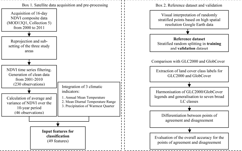
Multi-temporal datasets such as the MODIS product provide a cost-effective means to develop and to deliver regularly updated land cover products over large geographic regions [16–18]. Here we used as input features time series of 16-day NDVI composites from MODIS satellite sensor data (MOD13Q1) for the classification. For each of the 23 compositing periods, the average and the variance was derived from the full time series. The profile of average NDVI reflects the basic growth curves of different vegetation types. The variance reflects the class-specific reactivity to inter-annual changes in climatic driving variables (e.g., temperature, precipitation). Three climatic features were added to the NDVI-based features to facilitate large scale classifications with a common set of support vectors. The overall workflow is schematized in Figure 1.

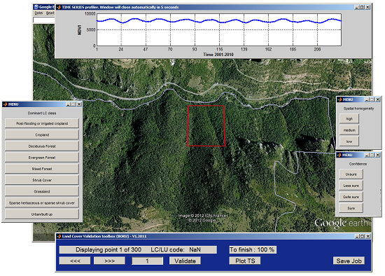
To reduce the efforts required for collecting ground truth information, reference data were derived through visual interpretation of high resolution images. For this purpose a Matlab (MathWorks) tool was developed making efficient use of GE data.

For the classification a Least Square Support Vector Machine (LS-SVM) algorithm, developed by Suykens et al. [19], was implemented. LS-SVM represents a variant of the original SVM formulation [20] with similar classification performance, reduced complexity and enhanced processing power [21]. We selected a SVM-based algorithm, as this method is used in various remote sensing classification problems and achieves good accuracy compared to other classification algorithms (e.g., maximum likelihood, discriminant analysis or decision trees). A comprehensive review is available in [22]. The classification performance of SVM with MODIS time series was assessed in [23]. The authors investigated, among other issues, the impact of training samples size and confirmed the superior generalization power even with small number of training samples (20 pixels per class). They also explored the variability in the overall accuracy using multiple randomly selected subsets of training samples, for a given training sample size.

In our study, we trained the LS-SVM algorithm with repeated random splits of the training dataset to select a small set of suitable support vectors optimizing class separability [24,25].

For comparison of our LS-SVM LC map with existing land cover products, validation focused on an independent dataset not used during the training phase. Class-specific and overall classification accuracies were calculated. Special attention was paid to those samples, where existing maps disagreed.

2.2. Satellite Data and Pre-Processing

The data used in this study consisted of 16-day NDVI composites from MODIS/Terra with a 250-m pixel size. The MODIS 16-day NDVI composite is a Level 3 product (MOD13Q1), calculated from the Level 2 daily surface reflectance product (MOD09 series) [26]. Data were aggregated using the Constrained View angle-Maximum Value Composite (CV-MVC) compositing method in a 16-day interval [27].

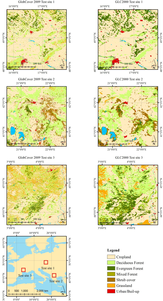
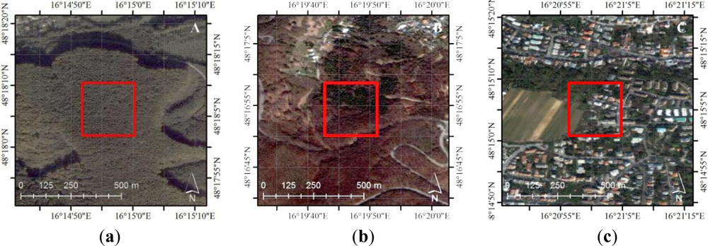
MODIS NDVI data spanning from February 2000 to mid-2011 were downloaded for three experimental test sites (

Table 2. Summary of the experimental test sites. The data used in this study consisted of 16-day Normalized Difference Vegetation Index (NDVI) composites for three test sites (2001 to 2010), from which averages and variances were calculated for each 16-day interval. Additionally, three climatic variables were used in the LC classification. Their respective average values are indicated.

Test Site	Lat./Lon.	Extension	MODIS Image Frame	Annual Mean Temperature (°C)	Mean Diurnal Range (°C)	Precipitation of Warmest Quarter (mm)
	(Scene Centre)	(km2)
Eastern Austria	48°52′6″N/18°13′44″E	107,400	h18v04	8.2	9.2	258
Macedonia	41°39′21″N/21°46′7″E	54,500	h18v04	9.7	10.2	137
Southern France	44°21′32″N/3°57′46″E	34,455	h19v04	10.3	9.8	186

). The test sites were selected to cover a variety of land cover types and climatic conditions in Europe.

MOD13Q1 image frames (here h18v04 and h19v04) were reprojected from the Sinusoidal to UTM projection with map datum WGS 84. This coordinate transformation was achieved using the MODIS data Reprojection Tool (MRT) with nearest neighbor resampling. The sub-setting of the three test sites was performed on the reprojected data. Images were consequently stacked to produce the time series dataset. One important requirement for multi-temporal analysis is the co-registration of the various acquisitions in the time series. According to the MODIS team, the geolocation accuracy is approximately 50 m at nadir [28]. Taking into account both nadir and off-nadir pixels, [17] reported an error of about 113 m that is considered acceptable for the purpose of the analysis.

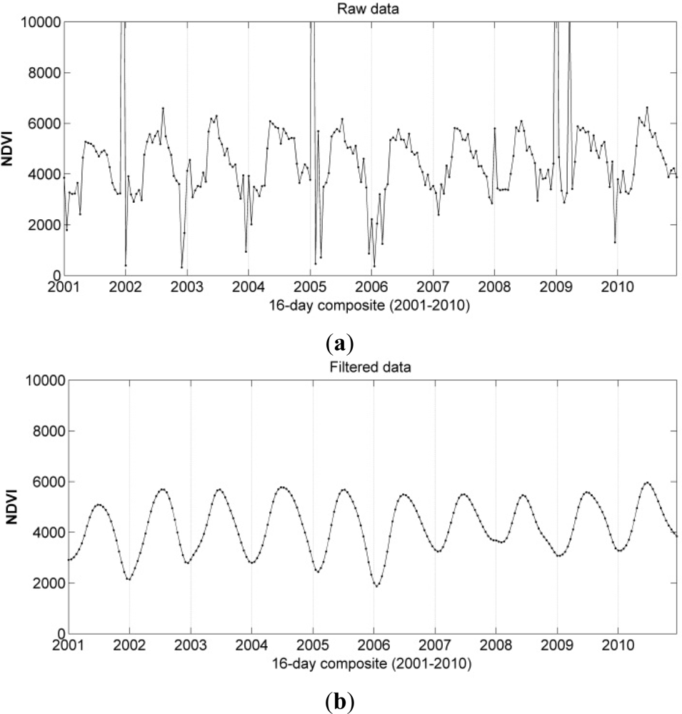
To fill data gaps, and to remove undesired effects of undetected clouds and poor atmospheric conditions, the time series data were filtered. The generation of the filtered dataset was based on a smoothing technique described in [29]. Data smoothing was achieved continuously from year 2000 to 2011. The employed Whittaker smoother [30] balances fidelity to the observations with the roughness of the smoothed curve. The algorithm is extremely fast, gives continuous control over smoothness with only one parameter, and interpolates automatically missing data. For further details the reader is referred to [29,31,32]. An example of NDVI time series before and after the filtering is presented in Figure 2.

The filtered time series consisted of 230 NDVI data values (10 years of data, 23 acquisitions per year, 1 observation every 16 days) from the start of 2001 to the end of 2010 (first and last complete year). The 230 NDVI data values were summarized to provide 16-day inter-annual averages (n = 23) and the corresponding variances (n = 23) for the period 2001–2010. The final NDVI dataset used in our study thus consisted of 46 observations representing the inter-annual averages and variances. A positive effect of using multi-annual data was shown by [33] where the effect of data compositing and length of the observation period on the LC accuracy was investigated.

As a consequence of the multi-annual data compositing, changes in land use and land cover may be expected to produce artefacts in the inter-annual averages (and variances) of the NDVI values. In this study, we assumed that LULC changes would have only a minimal impact on our European dataset. The rate of land cover changes for 36 European countries was estimated by [34] being 1.3% of the total land surface for the period 2000–2006, with average annual change rates of 0.08% for Austria, 0.14% for Macedonia and 0.11% for France.

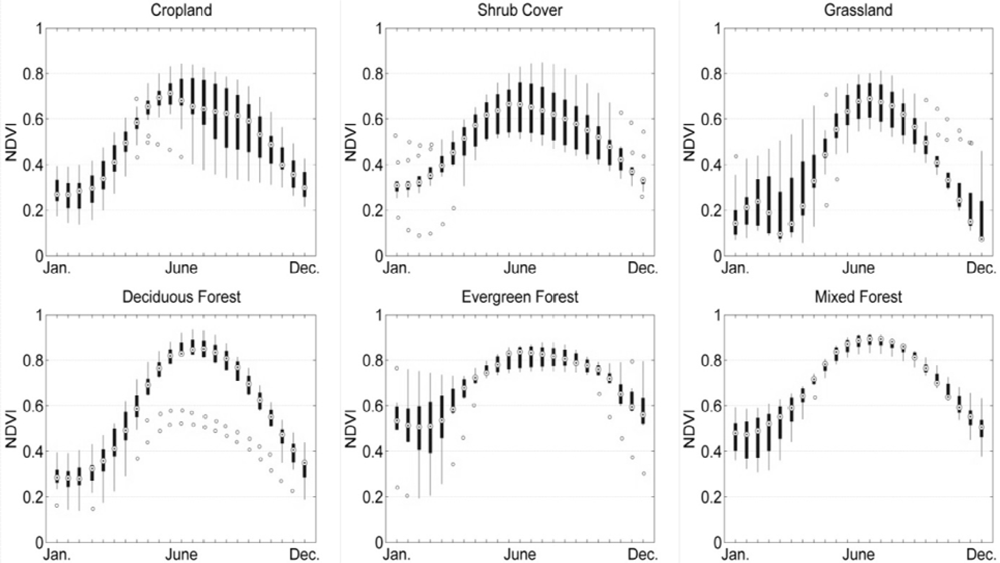
Three climatic indicators were included as LS-SVM input features so that the classifier receives information concerning the respective climatic conditions of each sample: the Annual Mean Temperature, the Mean Diurnal Temperature Range, and the Precipitation of Warmest Quarter calculated at 1-km spatial resolution. These three indicators were selected from the global climate layers of the WorldClim [35] dataset summarizing annual and seasonal trends of monthly temperature and rainfall values. Temperature and precipitation are important drivers of crop/vegetation growth and phenology. They are thus responsible for inter-annual and spatial variability of NDVI profiles.

The data values of the 49 features dataset were normalized using the standard score and constituted the input for the multi-temporal land cover (LS-SVM) classification.

2.3. Reference Dataset

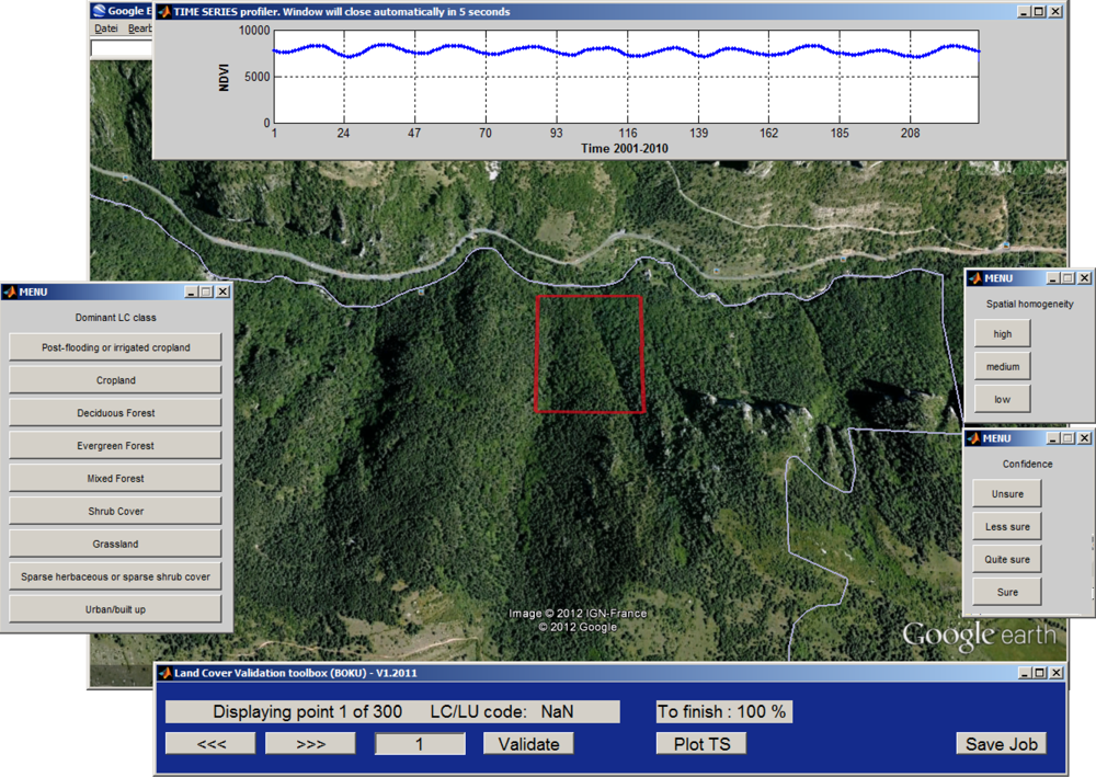
Reference LC information is required to train the LS-SVM, and to determine the quality of the established map in the accuracy assessment process. Visual interpretation of high spatial resolution images represents a time- and cost-saving alternative to traditional field surveys for ground truthing, and the only practical solution at regional and global scales [36,37]. For this purpose, a software toolbox was developed under Matlab to assist the display of satellite images available in GE and to add the visually determined LC label to each of the surveyed point. The NDVI time series corresponding to the MODIS 250-m pixel under validation was used to assess the consistency of the interpreted LC type with the temporal characteristics and to cross-check for changes that may have occurred during the 10 years. The main interface of the software toolbox is presented in Figure 3.

Two quality indicators were also assigned: (i) the confidence of interpretation, and (ii) the homogeneity of the area under interpretation. The first index categorizes the uncertainties arising while interpreting the high spatial resolution images. Four levels were distinguished: ‘Sure’, ‘Quite sure’, ‘Less sure’ and ‘Unsure’. The second index expresses the level of pixel homogeneity observed in the GE high spatial resolution images. We defined three possible categories based on the number and proportion of land cover types covering the MODIS 250-m pixel footprint and in its neighborhood area (about half a pixel to account for possible geolocation errors) (Figure 4):

• ‘High’ for homogeneous pixels containing only one land cover type (a);
• ‘Medium’ for mixed pixels with a clear predominance of one land cover type (b);
• ‘Low’ for mixed pixels with more than one land cover type without a clear majority (c). Note that despite this low homogeneity a (single) LC label was assigned.

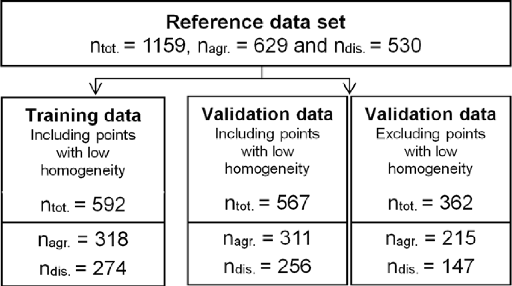
Using this approach, we visually interpreted a total number of 1,235 points randomly selected, of which 76 were qualified as ‘Unsure’. To reduce thematic errors in the reference dataset caused by the visual interpretation, these 76 points were excluded from further analysis.

The final dataset (n_tot = 1,159) was randomly split into two sub-samples (training and validation). For the optimization of the LS-SVM algorithm, only the training samples were used. The validation samples were used only for the classification performance assessment. Accuracy measures were calculated for different levels of pixel homogeneity: (1) first for medium to high homogeneity levels (n = 362), and (2) subsequently including all levels of pixel homogeneity (n = 567) .

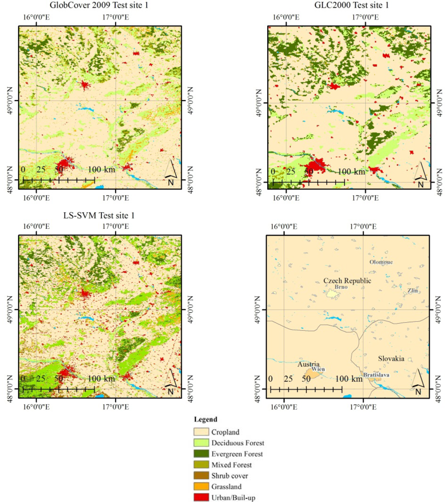
2.4. Comparison with Existing LC Products

The classification performance of the LS-SVM was compared to two existing LC products (GLC2000 and GlobCover). The LC class codes were extracted based on the exact location of the reference dataset points for GLC2000 (1-km pixel size). For GlobCover (300-m pixel size) a 3 × 3 neighborhood majority rule was used. In case where no class met the majority threshold, the center value was taken. A prerequisite to compare land cover data from existing LC products is the harmonization of the different classification legends. Processing aspects and recommendations for LC harmonization are described in [38]. Although GLC2000 and GlobCover are based on different mixed unit definitions and LC legends, both consider 22 LC classes according to the United Nations (UN) Land Cover Classification System (LCCS) [8]. Various methodologies have been proposed to aggregate and compare LC maps obtained from different satellite sensor data and mapping projects [37]. In our study, the LC legends of GLC2000 and GlobCover were first cross-related using a crisp approach [12]. This permits comparing class descriptions between the two mapping projects. Subsequently, the LC classes of the two legends were translated to a third system and thematically aggregated into seven LC classes (see Table 1). 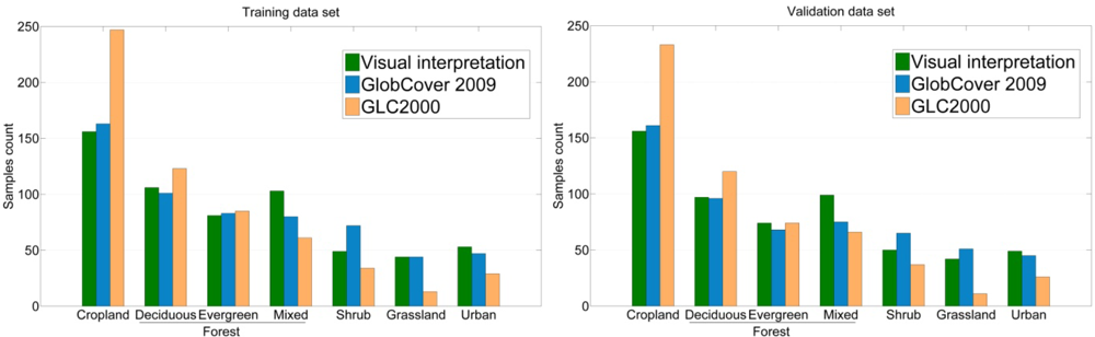This yields two new LC maps with harmonized legends (Figure 5). After harmonization and aggregation of legends, the areas of agreement (‘agr.’) and of disagreement (‘dis.’) between the two recoded LC products were derived. The distribution and the number of samples in the training and validation datasets are provided in Figure 6 and in Figure 7, respectively.

2.5. Classification Algorithm and Training Strategy

The image classification was performed by a non-linear SVM classifier [20]. The algorithm uses a kernel function to transform the training samples from the input space to a feature space of higher dimension. This results in a linearly separable dataset—normally non-linearly separable in the original input space—that can be separated by a linear classifier [39]. In this high-dimensional space, the algorithm finds an optimal separating hyperplane between two classes of training samples. The optimal hyperplane is constructed by maximizing the distance (margin) to the closest data points from the plane. The orientation of the plane is determined only by the training points that lie on the class boundaries, the so-called ‘support vectors’ [40].

SVMs are intrinsically binary classifiers and different strategies have been proposed to solve the multi-class problem [41,42]. However, various studies found that the performance of one approach compared to another depends on the dataset used and on the specific classification problem [43]. In this study, the multi-class classification problem was decomposed into multiple binary classifications using the one-against-one coding scheme, which provides good accuracy and is usually more suitable for practical use [44] compared to other coding schemes. This approach was also selected in similar studies dealing with land cover classification [45]. Regarding SVM algorithm and kernel function settings, we used a Least Square-SVM (LS-SVM) classifier with a Radial Basis Function (RBF) kernel. LS-SVM is a particular case of SVMs proposed by Suykens and Vandewalle [19,46]. 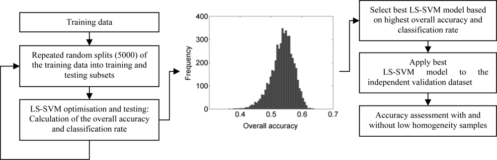The original formulation was revised to use a set of linear equations instead of quadratic programming problems and therefore to reduce the complexity and to improve the computing power [21]. The algorithm has two tuning parameters, namely the regularization parameter and the scaling factor of the kernel function. For the purpose of our study, the two tuning parameters and the optimum set of support vectors were optimized concurrently in a computational loop (5,000 iterations). In a first step, the training dataset was randomly split into subsets of training (candidate support vectors) and testing datasets. Based on these candidate support vectors (subset of training samples), a model optimization was performed to identify the best performing parameter combination for our classification problem. For this purpose, we used a grid-search method, as recommended by [47]. Each parameter combination was checked using a leave-one-out cross-validation, and the parameter pair with best cross-validation accuracy was selected. For each split, the LS-SVM model was optimized with the candidate support vectors, and the overall accuracy and the classification rate were assessed using the testing dataset. The number of candidate support vectors (80) was given by the minimum number of samples that each class has in the training set. This optimization was repeated 5,000 times using random splits of the training dataset into multiple subsets of training (candidate support vectors) and testing datasets. The best LS-SVM model of the 5,000 iterations was selected based on the highest overall accuracy and classification rate and it was applied to the independent validation dataset. Since random splitting was applied, some samples may never be selected, whereas others may be selected more than once. The schematization of the training, testing and validation process is presented in Figure 8. With this approach, we selected the most informative training samples that were likely to be good support vectors for the entire study region. The importance of small but informative training samples was also highlighted in previous studies dealing with intelligent selection of reference data for SVM classification in the spectral domain [24,25].

2.6. Accuracy Assessment and Accuracy Target

The classification performance evaluation was based on common statistical measures [48] derived from the classification error matrix. Only the validation dataset was used for this purpose. The selected statistical measures included the Overall Accuracy (OA), the Producer’s Accuracy (PA), the User’s Accuracy (UA), and the Cohen’s Kappa coefficient (κ). The two-side confidence intervals (CI) for the OA were calculated at 95% confidence level using the normal approximation method [49] with the continuity correction.

The performance of the LS-SVM classifier for the entire validation dataset is reported and distinguishing between ‘agr.’ and ‘dis.’ validation samples. Similarly, we report the accuracy of GlobCover and GLC2000. In benchmarking the LS-SVM performance, we refer to the classification accuracy achieved with GlobCover and GLC2000. We report the increase/decrease of the OA of LS-SVM classifier as percentage of the OA for GlobCover and for GLC2000. The statistical significance of the differences between the pairs LS-SVM-GlobCover and LS-SVM-GLC2000 was evaluated with the McNemar’s test with the continuity correction [50].

3. Results

3.1. Accuracy Assessment for Medium and High Homogeneity Samples

A first accuracy assessment was performed using only those samples qualified as medium to high homogeneity. Thus, the 205 low homogeneity samples (n_agr = 96 and n_dis = 109) were excluded (Figure 7). The error matrices and accuracy measures for LS-SVM, GlobCover and GLC2000 are presented in

Table 3. Error matrices and statistical measures for LS-SVM, GlobCover and GLC2000. Validation dataset excluding points of low spatial homogeneity (n_tot = 362). The error matrix was summarized based on the statistical measures: Producer’s Accuracy (PA), User’s Accuracy (UA), Overall Accuracy (OA) and the Cohen’s Kappa coefficient (κ). The visual interpretation of GE imagery was considered the ground truth (Reference).

		Reference							∑	P.A.	U.A.
		C	D	E	M	S	G	U
LS-SVM	Cropland (C)	88	3	4	0	11	8	0	114	81%	77%
	Deciduous Forest (D)	3	49	2	9	2	3	0	68	75%	72%
	Evergreen Forest (E)	2	4	28	19	0	0	0	53	68%	53%
	Mixed Forest (M)	2	6	7	33	0	0	0	48	53%	69%
	Shrub Cover (S)	9	1	0	1	17	3	1	32	53%	53%
	Grassland (G)	2	2	0	0	0	14	0	18	50%	78%
	Urban (U)	3	0	0	0	2	0	24	29	96%	83%
	∑	109	65	41	62	32	28	25	362	O.A.:	70%
										κ:	63%
		C	D	E	M	S	G	U	∑	P.A.	U.A.
GlobCover	Cropland (C)	74	8	2	3	8	7	2	104	68%	71%
	Deciduous Forest (D)	3	29	5	12	1	1	0	51	45%	57%
	Evergreen Forest (E)	3	3	26	11	0	2	0	45	63%	58%
	Mixed Forest (M)	0	9	6	35	3	1	0	54	56%	65%
	Shrub Cover (S)	23	3	2	0	19	1	0	48	59%	40%
	Grassland (G)	6	13	0	1	0	16	0	36	57%	44%
	Urban (U)	0	0	0	0	1	0	23	24	92%	96%
	∑	109	65	41	62	32	28	25	362	O.A.:	61%
										κ:	53%
		C	D	E	M	S	G	U	∑	P.A.	U.A.
GLC 2000	Cropland (C)	95	15	7	2	14	13	5	151	87%	63%
	Deciduous Forest (D)	9	34	3	12	3	5	0	66	52%	52%
	Evergreen Forest (E)	1	5	22	19	1	2	1	51	54%	43%
	Mixed Forest (M)	1	7	4	27	4	0	0	43	44%	63%
	Shrub Cover (S)	2	3	5	2	10	0	1	23	31%	43%
	Grassland (G)	1	1	0	0	0	8	0	10	29%	80%
	Urban (U)	0	0	0	0	0	0	18	18	72%	100%
	∑	109	65	41	62	32	28	25	362	O.A.:	59%
										κ:	20%

for the corresponding validation dataset (n_tot = 362).

LS-SVM achieved an overall accuracy (OA) of 70% (95% C.I.: 65%–75%) and an overall κ of 0.63; GlobCover and GLC2000 reported an OA of 61% (95% C.I.: 56%–66%) and of 59% (95% C.I.: 54%–64%), respectively. From these figures we calculated the percentage of increase or decrease of the overall accuracy of LS-SVM with respect to GlobCover and GLC2000. In this comparison, LS-SVM resulted 14% and 18% more accurate than GlobCover and GLC2000 respectively. According to the two-tailed P-value, differences are considered to be extremely statistically significant (p < 0.001).

Table 4. Summary table for validation data excluding points of low spatial homogeneity; the top part of the table shows the percentage of increase/decrease of overall accuracy (OA) for LS-SVM with respect to GlobCover and GLC2000. The bottom part of the table shows statistical significance of differences of the results based on the McNemar’s test (P-value and Chi-square) with the continuity correction. NS = Non-Significant result and S = Significant result at the 95% confidence level.

% Increase/Decrease OA of LS-SVM with Respect to:
	Total	Agreement	Disagreement
GlobCover	14%	5%	68%
GLC2000	18%		89%
	McNemar’s Test
	P-value
GlobCover	P < 0.001 (S)	P > 0.05 (NS)	P < 0.001 (S)
GLC2000	P < 0.001 (S)		P < 0.001 (S)
	Chi-square (df = 1)
GlobCover	7.46	0.68	22.72
GLC2000	9.69		27.48

shows a summary of the percentage of increase/decrease of the overall accuracy for LS-SVM with respect to GlobCover and GLC2000. An example of the three maps is provided in Figure 9 for a subset in test site 1.

In details, Cropland in LS-SVM reported a very high producer’s accuracy, indicating a good identification for all points visually interpreted as this class (Table 3); errors in the user’s accuracy were often due to confusion with Shrub Cover. This result indicates that LS-SVM produces an overestimation of Cropland class with a commission error of 23%. A similar trend was observed in GLC2000, with lower user’s accuracies due to an additional confusion of Cropland with Deciduous Forest and Grassland classes. In contrast, GlobCover presented a higher omission error (32%) due to confusion with Shrub Cover. The poor producer’s accuracy of Cropland in the GlobCover product was due to confusion with Deciduous Forest, Shrub Cover and Grassland. Amongst the three products, LS-SVM and GLC2000 gave the best results for the Cropland class.

For all LC products, Shrub Cover and Grassland were the two most difficult classes to identify with a producer’s accuracy ranging from 29% (GLC2000) to 59% (GlobCover) and a user’s accuracy ranging from 40% (GlobCover) up to 80% (GLC2000). All three LC products confused Shrub Cover and Grassland classes with Cropland; GLC2000 achieved the lowest performance (omission error 71%).

To better illustrate the difficulties encountered in classifying the mentioned LC classes, Figure 10 represents the average temporal NDVI profiles of the 6 vegetated LC classes present in the study region. The graph was generated plotting the NDVI of the selected support vectors (n = 80). NDVI temporal profiles clearly highlight the similarities in the signatures of Cropland and Shrub Cover classes and the resulting difficulties in separating Shrub Cover from Cropland. On the contrary, Grassland and Cropland present quite different temporal profiles. In the latter case, the misclassification might be partly due to errors in the visual interpretation of the high resolution images. Problems in separating these two classes are also commonly reported in other studies [11]. For instance, classification results of Shrub Cover and Grassland showed clear discrepancies with the interpretation of experts in the validation of GlobCover [9].

Regarding forest LC classes for LS-SVM, Deciduous Forest class was classified with producer’s and user’s accuracies greater than 70%. Evergreen Forest presented a lower accuracy with a producer’s accuracy of 68% and a user’s accuracy of 53%, being often confused with Mixed Forest class. The commission error indicates that LS-SVM produces an overestimation of Evergreen Forest class with an error of 47%. In both GlobCover and GLC2000, we observed a high commission error (42%–57%) for Evergreen Forest. Confusions between forest types were also observed in GlobCover, indicating that the temporal information was not optimally used. A source of error could lso be in the way the forest was interpreted by the visual interpreter. For instance, in the validation of GlobCover many forest points were often assigned directly to Mixed Forest class since leaf type and the leaf phenology information were not available [9]. A similar explanation was provided by [11] for the validation of GLC2000. A visual assessment showed that confusion between Deciduous Forest and Mixed Forest classes is also occurring in the LS-SVM LC map. For instance, a detailed analysis of the region presented in Figure 9 indicated that the Deciduous Forest areas located West of Vienna and North of Bratislava were confused with Mixed Forest.

Regarding Urban/Built-up class, all three LC products provided a good accuracy, with GlobCover achieving the best results. GLC2000 produced an omission error of 28% due to confusion of this class with Cropland.

3.2. Accuracy Assessment for All Levels of Pixel Homogeneity

A second accuracy assessment was undertaken considering all levels of pixel homogeneity (n_tot = 567) (Figure 7). In this case, the LS-SVM gave an OA of 63% (compared to 70% considering only medium-high homogeneity samples). Overall, the LS-SVM map was 10% and 24% more accurate compared to GlobCover and GLC2000, respectively.

The three LC products reported a similar overall accuracy (OA_agr of 64% for LS-SVM and 68% for GlobCover and GLC2000) where GlobCover and GLC2000 maps agreed. In the case of disagreement, GlobCover reported an OA_dis of 43% whereas GLC2000 showed significantly lower classification accuracy (OA_dis of 29%). LS-SVM gave for those samples an overall agreement (OA_dis) of 61%. A visual assessment indicated that the significantly lower performance of GLC2000 is probably caused by differences between the spatial resolutions of the LC map (1-km pixel size) and the spatial reference used for the visual interpretation (about 250-m). Due to this difference, two or more LC types could correspond to the same GLC2000 pixel (mixed pixel problem). This issue was expected to be more pronounced in areas with low homogeneity. This was the main reason for restricting the analysis in the previous section to samples of medium to high homogeneity.

3.3. Accuracy Assessment for Agreement and Disagreement Samples

To further investigate systematic patterns in classification performance, we evaluated the overall accuracy of the LS-SVM for samples where existing maps (GlobCover and GLC2000) agree or disagree. For this detailed analysis we considered only medium and high homogeneity samples (n_agr = 215 and n_dis = 147).

Error matrices and statistical measures are presented in

Table 5. Error matrices and statistical measures for LS-SVM and GlobCover/GLC2000 for the agreement data points (n_agr = 215).

		Reference							∑	P.A.	U.A.
		C	D	E	M	S	G	U
LS-SVM	Cropland (C)	59	3	3	0	3	4	0	72	81%	82%
	Deciduous Forest (D)	3	23	2	4	2	1	0	35	70%	66%
	Evergreen Forest (E)	1	2	18	10	0	0	0	31	67%	58%
	Mixed Forest (M)	2	4	4	22	0	0	0	32	59%	69%
	Shrub Cover (S)	6	0	0	1	7	2	1	17	54%	41%
	Grassland (G)	0	1	0	0	0	7	0	8	50%	88%
	Urban (U)	2	0	0	0	1	0	17	20	94%	85%
	∑	73	33	27	37	13	14	18	215	O.A.:	71%
										κ:	64%
		C	D	E	M	S	G	U	∑	P.A.	U.A.
GlobCover/GLC2000	Cropland (C)	69	5	1	1	4	5	1	86	95%	80%
	Deciduous Forest (D)	2	21	3	7	0	1	0	34	64%	62%
	Evergreen Forest (E)	1	1	18	7	0	1	0	28	67%	64%
	Mixed Forest (M)	0	6	3	22	2	0	0	33	59%	67%
	Shrub Cover (S)	1	0	2	0	7	0	0	10	54%	70%
	Grassland (G)	0	0	0	0	0	7	0	7	50%	100%
	Urban (U)	0	0	0	0	0	0	17	17	94%	100%
	∑	73	33	27	37	13	14	18	215	O.A.:	75%
										κ:	49%

for the samples in agreement. The overall accuracy was 71% (95% C.I.: 65%–77%) for LS-SVM and 75% (95% C.I.: 69%–81%) for GlobCover/GLC2000. The error was more uniformly distributed among all LC classes, with Cropland, Deciduous Forest and Urban being classes with best accuracies. Percentage differences between LS-SVM and the combination of GlobCover/GLC2000 are not considered statistically significant (p > 0.05) (see Table 4). Interestingly, where all three maps agreed (n = 144) we found an overall classification accuracy of 88%.

Table 6. Error matrices and statistical measures for LS-SVM and GlobCover/GLC2000 for the disagreement data points (n_dis = 147).

		Reference							∑	P.A.	U.A.
		C	D	E	M	S	G	U
LS-SVM	Cropland (C)	29	0	1	0	8	4	0	42	81%	69%
	Deciduous Forest (D)	0	26	0	5	0	2	0	33	81%	79%
	Evergreen Forest (E)	1	2	10	9	0	0	0	22	71%	45%
	Mixed Forest (M)	0	2	3	11	0	0	0	16	44%	69%
	Shrub Cover (S)	3	1	0	0	10	1	0	15	53%	67%
	Grassland (G)	2	1	0	0	0	7	0	10	50%	70%
	Urban (U)	1	0	0	0	1	0	7	9	100%	78%
	∑	36	32	14	25	19	14	7	147	O.A.:	68%
										κ:	61%
		C	D	E	M	S	G	U	∑	P.A.	U.A.
GlobCover	Cropland (C)	5	3	1	2	4	2	1	18	14%	28%
	Deciduous Forest (D)	1	8	2	5	1	0	0	17	25%	47%
	Evergreen Forest (E)	2	2	8	4	0	1	0	17	57%	47%
	Mixed Forest (M)	0	3	3	13	1	1	0	21	52%	62%
	Shrub Cover (S)	22	3	0	0	12	1	0	38	63%	32%
	Grassland (G)	6	13	0	1	0	9	0	29	64%	31%
	Urban (U)	0	0	0	0	1	0	6	7	86%	86%
	∑	36	32	14	25	19	14	7	147	O.A.:	41%
										κ:	32%
		C	D	E	M	S	G	U	∑	P.A.	U.A.
GLC 2000	Cropland (C)	26	10	6	1	10	8	4	65	72%	40%
	Deciduous Forest (D)	7	13	0	5	3	4	0	32	41%	41%
	Evergreen Forest (E)	0	4	4	12	1	1	1	23	29%	17%
	Mixed Forest (M)	1	1	1	5	2	0	0	10	20%	50%
	Shrub Cover (S)	1	3	3	2	3	0	1	13	16%	23%
	Grassland (G)	1	1	0	0	0	1	0	3	7%	33%
	Urban (U)	0	0	0	0	0	0	1	1	14%	100%
	∑	36	32	14	25	19	14	7	147	O.A.:	36%
										κ:	20%

reports the classification performance results for the disagreement data samples (n_dis = 147). It was not surprising that the overall accuracy decreased for this portion of the dataset. Nevertheless, LS-SVM still achieved an overall accuracy of 68% (95% C.I.: 60%–76%) while GlobCover and GLC2000 reported an overall accuracy of only 41% (95% C.I.: 33%–50%) and 36% (95% C.I.: 28%–44%), respectively. Compared to the validation dataset without the discrimination between agreement and disagreement, LM-SVM only showed a modest reduction in overall classification accuracy (from 70% to 68%). On the contrary, dramatic drops in overall classification accuracies were noted for GlobCover and GLC2000. For example, in the case of GlobCover, the overall classification accuracies dropped from 61% (Table 3) to 41% (Table 6).

Calculating the percentage of increase/decrease of the overall accuracy for the map pairs, we found that LS-SVM was 68% and 89% more accurate for the disagreement dataset compared to GlobCover and GLC2000, respectively. According to the two-tailed P-value (p < 0.001), differences are considered to be extremely statistically significant. A summary of the results is presented in Table 4.

4. Discussion

The results presented here demonstrate that there is a high potential in using LS-SVM fed with MODIS 250-m NDVI (16-day composites) and gridded climatic indicators for land cover classification. LS-SVM NDVI-derived LC maps achieved an overall accuracy of 70% and an overall κ of 0.63. Although the overall accuracy is below the 85% target, commonly referred as a minimum level for satellite-based LC product (70% per class accuracy) [51], our findings are comparable to those of previous studies dealing with similar LC classes [17,52,53]. Foody [54] suggested that a practical and realistic accuracy target should be defined for each particular application. For instance, in [53] the author reviewed several LC classification based on remotely sensed data and reported a mean overall accuracy of 76.19% (standard deviation = 15.59%) and a mean κ of 0.65 (standard deviation = 0.19) with about eight LC classes. Our results are in line with the output of this review paper. When comparing our results to the accuracy achieved by GlobCover and GLC2000 aggregated to seven LC classes, we observed that LS-SVM LC map clearly outperforms these two (global) land cover products.

According to our findings, we summarize the results as follows:

• Previous studies were often focused on the comparison of various LC datasets, to assess their strengths and weaknesses and to make the users and map developers aware of specific mapping problems [13]. Herold et al. [11] highlighted that a significant improvement in our global land cover mapping capacities can be achieved with a better accuracy for the areas of spatial disagreement among existing LC products. We attempted to achieve this improvement focusing especially on those areas where existing maps disagree. Our experimental results demonstrate that in the case of the LS-SVM LC classification, the accuracy of data points for areas of disagreement was notably improved up to 68% (considering a similar minimum mapping unit, such as LS-SVM at 250 m and GlobCover at 300 m) (see Table 4). On the contrary, an improvement for agreement points was difficult to achieve, confirming that currently available LC products are already relatively accurate in areas of agreement (71–75% in our assessment). Interestingly, data points (n = 144) that resulted in agreement in the three datasets (LS-SVM, GlobCover and GLC2000) achieved an overall accuracy of 88%.
• Only a few previous studies have independently evaluated the accuracy of LC products where existing maps agree/disagree [11,14]. These studies and our findings confirm that the classification accuracy of areas of agreement is systematically higher compared to areas where two (or more) maps disagree.
• Distinguishing between points of agreement and disagreement proved also helpful in the LS-SVM training process. Although not shown in this study, the iterative selection of support vectors drawn only from the agreement portion provided higher accuracy compared to the selection from the disagreement portion only. In the latter case, the LS-SVM achieved an OA of 73% (support vectors selected from the agreement portion only) vs. 67% (support vectors selected from the disagreement portion only) for the entire testing dataset. The OA was 70% (Table 3) when no distinction between agreement and disagreement is done in the training process. Our experimental results suggest that available LC products can be used to derive agreement/disagreement maps. These maps can be used as a kind of prior knowledge in classification projects to minimize and optimize sampling efforts through guided sampling in areas of agreement. Probably, points of agreement are also less prone to possible mis-assignments in the visual interpretation.
• We observe a clear relationship between accuracy, agreement/disagreement and pixel homogeneity. Considering, for example, the results of our visual interpretation for the entire reference dataset (n_tot = 1159) we notice a prevalence of cases in agreement compared to disagreement (434 vs. 307) for high and medium homogeneity levels. On the contrary, at low homogeneity level we observe fewer cases in agreement compared with disagreement (195 vs. 223).
• Large differences in the classification accuracy were also observed in respect to the confidence of interpretation. For examples, LS-SVM LC map achieved an OA of 63% for all levels of pixel homogeneity and confidence of interpretation (n = 567). This accuracy decreased to 47% when we considered ‘Less sure’ (n = 113) samples only; it increased to 62% and to 80% for ‘Quite sure’ (n = 328) and for ‘Sure’ (n = 126) samples, respectively. The impact of removing those samples that were flagged as ‘Unsure’ (76 in the reference dataset, 49 in the validation dataset) was not statistically significant. This confirms that classification accuracy is strongly related to the confidence of interpretation and possibly to the uncertainties in the reference dataset.
• A more detailed analysis of the classification accuracy extended to low homogeneity samples was limited by the differences between the spatial resolutions of GLC2000 and the spatial reference used for the visual interpretation. Due to this difference, two or more LC types could correspond to the same GLC2000 pixel. Hence, any direct comparison disfavors the GLC2000 dataset for those pixels. Including low homogeneity levels, the classification accuracy for LS-SVM was improved up to 40% (vs. 68% only for medium and high homogeneity samples) compared with GlobCover at 300 m. This aspect requires further investigation to confirm trends in disagreement at various levels of pixel homogeneity.
• The inclusion of the three climatic features contributed to reduce the standard deviation of the OA within the LS-SVM optimization step (5,000 iterations) and increased the classification rate (less unclassified pixels) (not shown). Together this stabilized the classification results. In this study, however, the improvement in overall accuracy was not statistically significant compared to not including climatic features (not shown). The contribution of climatic data may have a higher impact when working over (climatically) more diverse/larger areas, as otherwise phenological shifts may lead to mis-classifications.

5. Conclusions and Recommendations

This work evaluated the land cover (LC) classification performance of a least square support vector machine (LS-SVM) algorithm using Moderate-resolution Imaging Spectroradiometer (MODIS) 250 m Normalized Difference Vegetation Index (NDVI) time series. The classification performance was compared to the overall accuracies of two existing LC products (GlobCover and GLC2000). In particular, results were evaluated with respect to points in agreement and disagreement between GlobCover and GLC2000 using a harmonized legend with seven land cover classes. This disjoint analysis was performed to evaluate possible improvements in classification accuracy where existing maps are inconsistent (disagree).

The LS-SVM NDVI-derived LC map achieved an overall accuracy of 70% and it resulted 14% and 18% more accurate compared to GlobCover and GLC2000, respectively. The LS-SVM map was as accurate as existing LC maps in points of agreement (71–75% in our assessment), while classification accuracy was significantly improved (from 36–41% to 68%) in points of disagreement. This improvement was as high as 68% considering a similar minimum mapping unit such as LS-SVM at 250-m and GlobCover at 300-m. Results showed that there is a high potential to significantly improve the accuracy for areas where existing products disagree. Within our 3 test sites, areas of disagreement represent roughly 35% of the total area. This opens new possibilities to revise existing LC maps (e.g., by focusing on areas of disagreement).

Additionally, we investigated the possibility to reduce the effort for visual interpretation. This can be done by selecting and interpreting only points of agreement. Points of disagreement could be excluded a-priori from the visual interpretation and from the training dataset because these points can be considered of low quality and little help for classification. In training the classification algorithm, one can exclusively rely on training samples extracted over points of agreement, thus reducing the effort required for visual interpretation (saving man power and time). In future studies, sampling effort can thus be reduced focusing only on areas of agreement.

Given the currently available global datasets, the users of LC products should in our opinion focus on combining existing maps and identify areas of agreement and disagreement. The accuracy of areas of spatial disagreement could then be improved based for example on the methodology proposed in this study. The proposed methodology can be easily generalized to different legend definitions or levels of land cover detail. This will help maximizing the overall accuracy of the resulting final land cover map as confirmed by our study.

Similar to several other studies [6,12,13,15], our work confirmed that there is no clear preference of one LC product compared to others. A selection will always have to be based on a specific purpose or application. Steps to further improve the accuracy of land cover maps include, for instance, ensembles of different algorithms for map production based on multi-source datasets [55]. Subsequently, these maps can be combined and synthetized in one product based on decision fusion rules [56,57].

References

1. Poulter, B.; Frank, D.C.; Hodson, E.L.; Zimmermann, N.E. Impacts of land cover and climate data selection on understanding terrestrial carbon dynamics and the CO2 airborne fraction. Biogeosciences 2011, 8, 2027–2036. [Google Scholar]
2. Sellers, P.J.; Dickinson, R.E.; Randall, D.A.; Betts, A.K.; Hall, F.G.; Berry, J.A.; Collatz, G.J.; Denning, A.S.; Mooney, H.A.; Nobre, C.A.; Sato, N.; Field, C.B.; Henderson-Sellers, A. Modeling the Exchanges of energy, water, and carbon between continents and the atmosphere. Science 1997, 275, 502–509. [Google Scholar]
3. Kastens, J.H.; Kastens, T.L.; Kastens, D.L.A.; Price, K.P.; Martinko, E.A.; Lee, R.Y. Image masking for crop yield forecasting using AVHRR NDVI time series imagery. Remote Sens. Environ 2005, 99, 341–356. [Google Scholar]
4. Lunetta, R.S.; Knight, J.F.; Ediriwickrema, J.; Lyon, J.G.; Worthy, L.D. Land-cover change detection using multi-temporal MODIS NDVI data. Remote Sens. Environ 2006, 105, 142–154. [Google Scholar]
5. Schneider, A.; Friedl, M.A.; Potere, D. Mapping global urban areas using MODIS 500-m data: New methods and datasets based on ‘urban ecoregions’. Remote Sens. Environ 2010, 114, 1733–1746. [Google Scholar]
6. Fritz, S.; See, L.; McCallum, I.; Schill, C.; Obersteiner, M.; van der Velde, M.; Bottcher, H.; Havlik, P.; Achard, F. Highlighting continued uncertainty in global land cover maps for the user community. Environ. Res. Lett 2011, 6, 044005. [Google Scholar]
7. Mayaux, P.; Eva, H.; Gallego, J.; Strahler, A.H.; Herold, M.; Agrawal, S.; Naumov, S.; Demiranda, E.E.; Dibella, C.M.; Ordoyne, C.; Kopin, I.; Roy, P.S. Validation of the Global Land Cover 2000 map. IEEE Trans. Geosci. Remote Sens 2006, 44, 1728–1739. [Google Scholar]
8. Di Gregorio, A.; Jansen, L.J.M. Land Cover Classification System (LCCS): Classification Concepts and User Manual; FAO Land and Water Development Division: Rome, Italy, 2000. [Google Scholar]
9. Bontemps, S.; Defourny, P.; Van Bogaert, E.; Arino, O.; Kalagirou, V.; Ramos Perez, J. GLOBCOVER 2009 Product—Description and Validation Report V. 2.2; Université Catholique de Louvain (UCL) & European Space Agency (ESA), 2011. Available online: http://ionia1.esrin.esa.int/ (accessed on 8 June 2011).
10. Friedl, M.A.; Sulla-Menashe, D.; Tan, B.; Schneider, A.; Ramankutty, N.; Sibley, A.; Huang, X. MODIS Collection 5 global land cover: Algorithm refinements and characterization of new datasets. Remote Sens. Environ 2010, 114, 168–182. [Google Scholar]
11. Herold, M.; Mayaux, P.; Woodcock, C.E.; Baccini, A.; Schmullius, C. Some challenges in global land cover mapping: An assessment of agreement and accuracy in existing 1-km datasets. Remote Sens. Environ 2008, 112, 2538–2556. [Google Scholar]
12. Kaptué, T.A.T.; Roujean, J.L.; De Jong, S.M. Comparison and relative quality assessment of the GLC2000, GLOBCOVER, MODIS and ECOCLIMAP land cover data sets at the African continental scale. Int. J. Appl. Earth Obs. Geoinf 2011, 13, 207–219. [Google Scholar]
13. Pflugmacher, D.; Krankina, O.N.; Cohen, W.B.; Friedl, M.A.; Sulla-Menashe, D.; Kennedy, R.E.; Nelson, P.; Loboda, T.V.; Kuemmerle, T.; Dyukarev, E.; Elsakov, V.; Kharuk, V.I. Comparison and assessment of coarse resolution land cover maps for Northern Eurasia. Remote Sens. Environ 2011, 115, 3539–3553. [Google Scholar]
14. Fritz, S.; See, L. Identifying and quantifying uncertainty and spatial disagreement in the comparison of global land cover for different applications. Global Change Biol 2008, 14, 1057–1075. [Google Scholar]
15. Jung, M.; Henkel, K.; Herold, M.; Churkina, G. Exploiting synergies of global land cover products for carbon cycle modeling. Remote Sens. Environ 2006, 101, 534–553. [Google Scholar]
16. Pfeifer, M.; Disney, M.; Quaife, T.; Marchant, R. Terrestrial ecosystems from space: A review of earth observation products for macroecology applications. Global Ecol. Biogeogr 2012, 21, 603–624. [Google Scholar]
17. Knight, J.F.; Lunetta, R.S.; Ediriwickrema, J.; Khorrarn, S. Regional scale land cover characterization using MODIS-NDVI 250 m multi-temporal imagery: A phenology-based approach. GISci. Remote Sens 2006, 43, 1–23. [Google Scholar]
18. Clerici, N.; Weissteiner, C.J.; Gerard, F. Exploring the use of MODIS NDVI-based phenology indicators for classifying forest general habitat categories. Remote Sens 2012, 4, 1781–1803. [Google Scholar]
19. Suykens, J.A.K.; Vandewalle, J. Least squares support vector machine classifiers. Neural Process. Lett 1999, 9, 293–300. [Google Scholar]
20. Vapnik, V. The Nature of Statistical Learning Theory; Springer-Verlag: New York, NY, USA, 1995. [Google Scholar]
21. Van Gestel, T.; Suykens, J.A.K.; Baesens, B.; Viaene, S.; Vanthienen, J.; Dedene, G.; de Moor, B.; Vandewalle, J. Benchmarking Least squares support vector machine classifiers. Mach. Learn 2004, 54, 5–32. [Google Scholar]
22. Mountrakis, G.; Im, J.; Ogole, C. Support vector machines in remote sensing: A review. ISPRS J. Photogramm 2011, 66, 247–259. [Google Scholar]
23. Shao, Y.; Lunetta, R.S. Comparison of support vector machine, neural network, and CART algorithms for the land-cover classification using limited training data points. ISPRS J. Photogramm 2012, 70, 78–87. [Google Scholar]
24. Foody, G.M.; Mathur, A. Toward intelligent training of supervised image classifications: Directing training data acquisition for SVM classification. Remote Sens. Environ 2004, 93, 107–117. [Google Scholar]
25. Wang, J.; Neskovic, P.; Cooper, L.N. Selecting Data for Fast Support Vector Machine Training. In Trends in Neural Computation (Studies in Computational Intelligence); Springer-Verlag: Berlin, Germany, 2007; Volume 35, pp. 61–84. [Google Scholar]
26. Vermote, E.F.; El Saleous, N.Z.; Justice, C.O. Atmospheric correction of MODIS data in the visible to middle infrared: First results. Remote Sens. Environ 2002, 83, 97–111. [Google Scholar]
27. Huete, A.; Didan, K.; Miura, T.; Rodriguez, E.P.; Gao, X.; Ferreira, L.G. Overview of the radiometric and biophysical performance of the MODIS vegetation indices. Remote Sens. Environ 2002, 83, 195–213. [Google Scholar]
28. Wolfe, R.E.; Nishihama, M.; Fleig, A.J.; Kuyper, J.A.; Roy, D.P.; Storey, J.C.; Patt, F.S. Achieving sub-pixel geolocation accuracy in support of MODIS land science. Remote Sens. Environ 2002, 83, 31–49. [Google Scholar]
29. Atzberger, C.; Eilers, P.H.C. Evaluating the effectiveness of smoothing algorithms in the absence of ground reference measurements. Int. J. Remote Sens 2011, 32, 3689–3709. [Google Scholar]
30. Eilers, P.H.C. A perfect smoother. Anal. Chem 2003, 75, 3631–3636. [Google Scholar]
31. Atzberger, C.; Eilers, P.H.C. A time series for monitoring vegetation activity and phenology at 10-daily time steps covering large parts of South America. Int. J. Digit. Earth 2011, 4, 365–386. [Google Scholar]
32. Atkinson, P.M.; Jeganathan, C.; Dash, J.; Atzberger, C. Inter-comparison of four models for smoothing satellite sensor time-series data to estimate vegetation phenology. Remote Sens. Environ 2012, 123, 400–417. [Google Scholar]
33. Huettich, C.; Herold, M.; Wegmann, M.; Cord, A.; Strohbach, B.; Schmullius, C.; Dech, S. Assessing effects of temporal compositing and varying observation periods for large-area land-cover mapping in semi-arid ecosystems: Implications for global monitoring. Remote Sens. Environ 2011, 115, 2445–2459. [Google Scholar]
34. Meiner, A.; Georgi, B.; Petersen, J.-E.; Uhel, R. Land Use—SOER 2010 Thematic Assessment (The European Environment—State and Outlook 2010); European Environment Agency: Luxembourg, 2010. [Google Scholar]
35. Hijmans, R.J.; Cameron, S.E.; Parra, J.L.; Jones, P.G.; Jarvis, A. Very high resolution interpolated climate surfaces for global land areas. Int. J. Climatol 2005, 25, 1965–1978. [Google Scholar]
36. Cihlar, J.L. Cover mapping of large areas from satellites: Status and research priorities. Int. J. Remote Sens 2000, 21, 1093–1114. [Google Scholar]
37. Strahler, A.; Boschetti, L.; Foody, G.; Friedl, M.; Hansen, M.; Herold, M.; Mayaux, P.; Morisette, J.; Stehman, S.; Woodcock, C. Global Land Cover Validation: Recommendations for Evaluation and Accuracy Assessment of Global Land Cover Maps; Office for Official Publications of the European Communities: Luxembourg, 2006. [Google Scholar]
38. Jansen, L.J.M.; Groom, G.; Carrai, G. Land-cover harmonisation and semantic similarity: Some methodological issues. Land Use Sci 2008, 3, 131–160. [Google Scholar]
39. Huang, C.; Davis, L.S.; Townshend, J.R.G. An assessment of support vector machines for land cover classification. Int. J. Remote Sens 2002, 23, 725–749. [Google Scholar]
40. Mathur, A.; Foody, G. Multiclass and binary SVM classification: Implications for training and classification users. IEEE Geosci. Remote Sens. Lett 2008, 5, 241–245. [Google Scholar]
41. Melgani, F.; Bruzzone, L. Classification of hyperspectral remote sensing images with support vector machines. IEEE Trans. Geosci. Remote Sens 2004, 42, 1778–1790. [Google Scholar]
42. Gualtieri, J.A. The Support Vector Machine (SVM) Algorithm for Supervised Classification of Hyperspectral Remote Sensing Data. In Kernel Methods for Remote Sensing Data Analysis; Camps-Valls, G., Bruzzone, L., Eds.; John Wiley & Sons, Ltd: New York, NY, USA, 2009; pp. 49–83. [Google Scholar]
43. Duan, K.B.; Keerthi, S. Which is the Best Multiclass SVM Method? An Empirical Study. In Multiple Classifier Systems (Lecture Notes in Computer Science); Oza, N.C., Polikar, R., Josef Kittler, J., Roli, F., Eds.; Springer: Berlin/Heidelberg, Germany, 2005; pp. 278–285. [Google Scholar]
44. Hsu, C.W.; Lin, C.J. A comparison of methods for multi-class support vector machines. IEEE Trans. Neural Networks 2002, 13, 415–425. [Google Scholar]
45. Kavzoglu, T.; Colkesen, I. A kernel functions analysis for support vector machines for land cover classification. Int. J. Appl. Earth Obs. Geoinf 2009, 11, 352–359. [Google Scholar]
46. Suykens, J.A.K.; van Gestel, T.; De Brabanter, J.; de Moor, B.; Vandewalle, J. Least Squares Support Vector Machines; World Scientific Pub.Co.: Singapore, 2002. [Google Scholar]
47. Hsu, C.W.; Chang, C.C.; Lin, C.J. A Practical Guide to Support Vector Classsification. Available online: http://www.csie.ntu.edu.tw/~cjlin/papers/guide/guide.pdf (accesed on 9 August 2012).
48. Foody, G.M. Status of land cover classification accuracy assessment. Remote Sens. Environ 2002, 80, 185–201. [Google Scholar]
49. Brown, L.; Cai, T.; DasGupta, A. Interval estimation for a binomial proportion. Stat. Sci 2001, 16, 101–117. [Google Scholar]
50. Siegel, S. Nonparametric Statistics for the Behavioral Sciences; McGraw-Hill: New York, NY, USA, 1956. [Google Scholar]
51. Thomlinson, J.R.; Bolstad, P.V.; Cohen, W.B. Coordinating methodologies for scaling landcover classifications from site-specific to global: Steps toward validating global map products. Remote Sens. Environ 1999, 70, 16–28. [Google Scholar]
52. Lotsch, A.; Tian, Y.; Friedl, M.A.; Myneni, R.B. Land cover mapping in support of LAI and FPAR retrievals from EOS-MODIS and MISR: Classification methods and sensitivities to errors. Int. J. Remote Sens 2003, 24, 1997–2016. [Google Scholar]
53. Wilkinson, G.G. Results and implications of a study of fifteen years of satellite image classification experiments. IEEE Trans. Geosci. Remote Sens 2005, 43, 433–440. [Google Scholar]
54. Foody, G.M. Harshness in image classification accuracy assessment. Int. J. Remote Sens 2008, 29, 3137–3158. [Google Scholar]
55. Benediktsson, J.; Chanussot, J.; Fauvel, M. Multiple Classifier Systems in Remote Sensing: From Basics to Recent Developments. In MCS’07 Proceedings of the 7th International Conference on Multiple Classifier Systems; Haindl, M., Kittler, J., Roli, F., Eds.; Springer-Verlag: Berli/Heidelberg, Germany, 2007; Volume 4472, pp. 501–512. [Google Scholar]
56. Waske, B.; Benediktsson, J.A. Fusion of Support Vector Machines for classification of multisensor data. IEEE Trans. Geosci. Remote Sens 2007, 45, 3858–3866. [Google Scholar]
57. Udelhoven, T.; van der Linden, S.; Waske, B.; Stellmes, M.; Hoffmann, L. Hypertemporal classification of large areas using decision fusion. IEEE Geosci. Remote Sens. Lett 2009, 6, 592–596. [Google Scholar]
Figure 1. Workflow of the proposed land cover classification and validation process. The description of satellite data acquisition and pre-processing is reported in Box 1. Box 2 presents the processing of the reference dataset and the comparison with GLC2000 and GlobCover.
Remotesensing 04 03143f1
Figure 2. Example of NDVI time series before (a) and after (b) filtering. Data smoothing was achieved continuously from year 2000 to 2011 using the Whittaker smoother (λ = 15). For the classification only data from 2001 to the end of 2010 was used and is shown in the graphs.
Remotesensing 04 03143f2
Figure 3. The software toolbox interface developed to assist the display of satellite images available in Google Earth (GE) and for adding the visually determined LC labels to each of the surveyed points. The software allows the interactive display of NDVI time series (2001–2010) corresponding to the MODIS 250-m pixel under validation (red box). Two panels are available to provide quality indicators (Confidence and Spatial homogeneity).
Remotesensing 04 03143f3
Figure 4. Illustration of different levels of pixel homogeneities. Examples are provided for Deciduous Forest (a), Deciduous Forest mixed with Evergreen Forest (b) and Urban mixed with Deciduous Forest and Cropland (c) LC classes as interpreted in the high resolution Google Earth images. (a) high homogeneity, (b) medium homogeneity, and (c) low homogeneity.
Remotesensing 04 03143f4
Figure 5. GLC2000 and GlobCover maps after legend aggregation for the three test sites.
Remotesensing 04 03143f5
Figure 6. Distribution of LC data for the training (left) and validation (right) dataset. The randomized division of reference samples into training (n = 592) and validation data (n = 567) was done by class.
Remotesensing 04 03143f6
Figure 7. The reference dataset was divided into training and validation subset. The total number of points and the corresponding agreement (‘agr’) and disagreement (‘dis’) are provided for each subset. The accuracy assessment stage distinguished between two validation datasets; one including the points with low homogeneity and one excluding these points.
Remotesensing 04 03143f7
Figure 8. The schematization of the LS-SVM training, testing and validation process. The best set of support vectors was selected using an iterative approach with repeated random splits of the training data into multiple training and testing subsets. For each iteration, the LS-SVM was trained with the candidate support vectors (training subset), and the accuracy and classification rate were assessed using the testing subset. The best LS-SVM model was selected from the 5,000 candidate models according to the highest overall accuracy and the best classification rate. This model was applied to the validation dataset for accuracy assessment.
Remotesensing 04 03143f8
Figure 9. Examples of GlobCover, GLC2000 and LS-SVM maps for a small region between the cities of Vienna (Austria), Bratislava (Slovakia) and Brno (Czech Republic).
Remotesensing 04 03143f9
Figure 10. NDVI temporal profiles of the six vegetated land cover classes considered in this study. The graph was generated plotting the 10-year average NDVI of pixels corresponding to selected training points (n = 80) used in final LS-SVM model optimization. Whiskers extend within 1.5 times the interquartile range from the ends of the box. Points beyond the whiskers are outliers.
Remotesensing 04 03143f10