Estimating Coastal Lagoon Tidal Flooding and Repletion with Multidate ASTER Thermal Imagery

Department of Geography, East Carolina University, Greenville, NC 27858, USA
Remote Sens. 2012, 4(10), 3110-3126; https://doi.org/10.3390/rs4103110
Submission received: 19 August 2012
/
Revised: 10 October 2012
/
Accepted: 12 October 2012
/
Published: 18 October 2012
(This article belongs to the Special Issue Thermal Remote Sensing Applications: Present Status and Future Possibilities)
Abstract
:Coastal lagoons mix inflowing freshwater and tidal marine waters in complex spatial patterns. This project sought to detect and measure temperature and spatial variability of flood tides for a constricted coastal lagoon using multitemporal remote sensing. Advanced Spaceborne Thermal Emission Radiometer (ASTER) thermal infrared data provided estimates of surface temperature for delineation of repletion zones in portions of Chincoteague Bay, Virginia. ASTER high spatial resolution sea-surface temperature imagery in conjunction with in situ observations and tidal predictions helped determine the optimal seasonal data for analyses. The selected time series ASTER satellite data sets were analyzed at different tidal phases and seasons in 2004–2006. Skin surface temperatures of ocean and estuarine waters were differentiated by flood tidal penetration and ebb flows. Spatially variable tidal flood penetration was evaluated using discrete seed-pixel area analysis and time series Principal Components Analysis. Results from these techniques provide spatial extent and variability dynamics of tidal repletion, flushing, and mixing, important factors in eutrophication assessment, water quality and resource monitoring, and application of hydrodynamic modeling for coastal estuary science and management.

1. Introduction
Coastal lagoons are prominent features along many of the worlds sandy coasts and form behind baymouth barriers, barrier spits and barrier islands. Barrier islands and lagoons compose a substantial extent of the world’s coastlines, and some type of barrier system borders nearly half of the United States coast. These stretches of islands and backbarriers are broken by tidal inlets of variable extent, and volumetric exchange between riverine, estuarine, and marine waters. Kjerfve and Magill (1989) [1] are widely recognized as noting that inlet characteristics strongly influence the exchange between tidal lagoons and the sea and found that backbarrier coastal lagoons could be characterized as “leaky,” “constricted,” or “choked,” based on inlet width and spacing. Along much of the east coast of the United States, lagoons are constricted with one dominant inlet. Constricted inlets effectively function as tidal drains that induce turbulence during flood and ebb exchanges such that tidal exchanges in coastal lagoons have been used to evaluate flushing characteristics through the use of hypsometry and hydraulic turn over [2–4]. In well-mixed coastal lagoons, hydraulic turn over time is expressed as the number of tidal cycles required to exchange all of the water in the basins [1,5,6]. It is a mathematical computation, which utilizes the total capacity of a basin and material “newly” injected into a basin. As such, it is of general use and is not appropriate for pathways or residence time of specific water parcels in the system.
Published works applying the Advanced Spaceborne Thermal Emission Radiometer (ASTER) and other multitemporal satellite observations have focused on various coastal or lacustrine environments, including stereoscopic observations of waves and wakes [7] and currents and fronts [8]. In thermal remote sensing, there have also been analyses specifically to develop thermal emissivity and temperature estimates for ASTER [9] and for monitoring volcanic lake craters [10]. Spatial dynamics of coastal waters and riverine discharges have been examined using satellite data [11], and time series Landsat thermal infrared (TIR) have also been used to assess coastal sea surface temperature variability and climatology [12,13] and effects of spatial resolution on detection of stream discharges [14]. However, published studies are lacking that investigate tidal zonation, flushing, repletion, or thermal IR dynamics of lagoons or inlets. In addition, Laymon and Quattrochi [15] note that, as compared with Landsat or coarser resolution satellites, ASTER provides higher spatial resolution thermal data, which could improve the estimation of surface energy fluxes. In a study of spatial and temporal variability of land surface temperature in Egypt, Miliaresis et al. [16] investigated multi-temporal Moderate Resolution Imaging Spectrometer (MODIS) data and elevation. Their results showed that coastal areas were distinguished by thermal segmentation into a unique spatial zone. Given the importance of lagoonal and estuarine environments in coastal habitat, primary production, and human development, the management of these regions could be served by a closer examination by applied thermal remote sensing.
The purpose of this study is to evaluate the potential for remote sensing of water exchange in well-mixed coastal lagoons using satellite thermal infrared (TIR) satellite observations. Of primary interest is the identification of patterns of tidal basin flooding and refilling with tidal exchange and the utility of such synoptic observations to coastal managers. Basin refilling (or repletion) occurs as a turbulent flow of irregular topography of lagoon floors. It was expected that thermal infrared observations could reveal the spatial extent and degree of penetration of coastal marine waters into a coastal lagoon that would otherwise be indistinct in multispectral wavelengths. Thus, the project seeks to apply remote sensing to reveal a pattern of “repletion footprint.” For the purpose of distinguishing water that is not exchanged from the basin to the ocean at low tide, the term “residual water” is applied. This exploration focuses on the tidal flushing capabilities of the ASTER sensor onboard Terra satellite, which offers the potential for observing at-satellite radiance temperature and possible derivation of skin sea surface temperature. While not a replacement for high-resolution hydrodynamic modeling and its capability to predict flushing, repletion, turnover, and residence time, the use of satellite TIR imagery would enable a synoptic perspective at low cost for continual environmental monitoring. For small coastal bays and barrier island fronted estuaries with dynamic tidal inlets, this could afford a very advantageous management tool.
2. Study Area
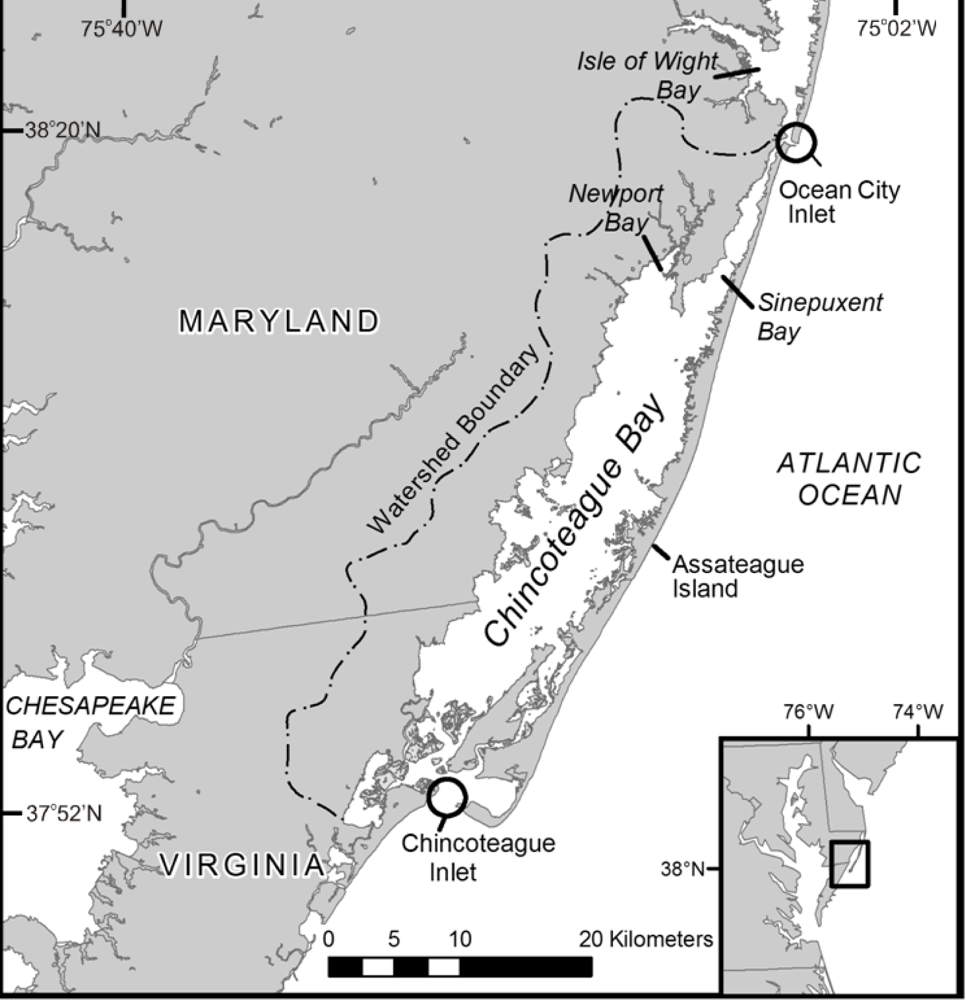
Chincoteague Bays offers an exemplary case study for understanding the complex interactions of land use and estuarine and lagoonal health, with a wide range of available coastal science observations [17]. Chincoteague Bay is located on the central Atlantic coast of the Delmarva Peninsula, astride the Virginia/Maryland border. The bay is enclosed to the east by Assateague Island and west by the upland of the Delmarva Peninsula (Figure 1). The bay is connected to the ocean via Chincoteague Inlet, the focus of this study in the south, and Ocean City Inlet to the north, via adjoining Sinepuxent Bay. Chincoteague Bay is surrounded by a relatively undeveloped watershed and is cleansed moderately by flushing from both inlets. Environmental conditions of Chincoteague Bay include historically extensive seagrasses and relatively good overall water quality with the exception of increasing localized eutrophication. Considered one of the most pristine coastal bays of the Mid-Atlantic, Chincoteague Bay is surrounded by a relatively undeveloped watershed and is cleansed moderately by flushing from both inlets [17,18].
The National Estuarine Eutrophication Assessment (1999) [19] estimated that overall microtidal amplitude for Chincoteague Bay averages 0.5 m, flushing volume 167,500,000 m3, and daily tide volume 323,671,498 m3, with a tide ratio = 0.26, and stratification = 0.00128. However, the volumetric contribution of deep channels near inlets and the intrinsic “choke-effect” of flood tidal marsh deltas yield slow flushing (∼63 days near Chincoteague, NEEA 2007) [20]. Although coarse data allows synoptic intercomparisons among bays, individual characteristics including watershed development, and inlet dynamics in other bays frequently yield much poorer water quality and hence, ecosystem vitality (e.g., Ocean City Bay and Isle of Wight Bay, MD, USA and Lynnhaven Bay, VA, USA). Generally good water quality, as evidenced by low nutrient levels, high clarity and low algal concentrations, has been found by monitoring in Chincoteague Bay, primarily in proximity of more frequently flushed inlets. Very good water quality (low nitrogen, moderate phosphorus, and very good clarity) can be found in association with flushing near Chincoteague Inlet, while interior Newport Bay and its upstream tributary exhibit high to very high algal concentrations, high phosphorus loading, low water clarity (measured by secchi disk depth), and low dissolved oxygen levels. Tributaries in the upper portions of this bay have degraded benthic communities and suffer an absence of submerged aquatic vegetation (SAV). Trends reported by the NEEA 2007 update [20] however, have raised concerns that water quality may be declining (and dissolved nitrogen increasing) in Chincoteague Bay, with diffuse nutrient loading and loss of SAV both symptomatic and negative feedbacks on future degradation of water quality.
3. Methodology
3.1. ASTER Quicklook Image Analysis
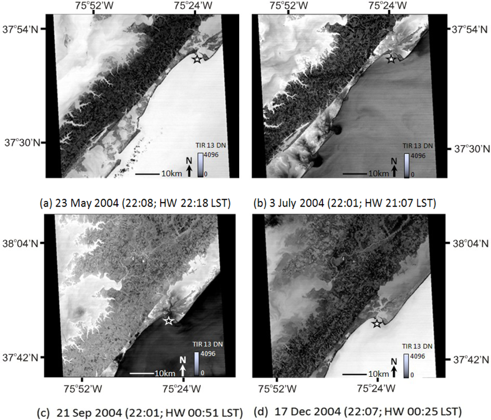
ASTER thermal infrared (TIR) satellite data was searched in the US Geological Survey Global Visualization Viewer (GLOVIS) ( http://glovis.usgs.gov/). Exploration of the image archive focused the imagery search on nighttime ASTER observations, since cloud-free images were more abundant and often higher thermal contrast between land and water features than daylight imagery. Although Landsat-7 ETM+ TIR imagery would be applicable, prior searches of available archives only uncovered limited and rather extensively cloud-covered data during the focal study period. For ASTER data, cloud-free flags and Quicklook images were examined for over 200 images, with tidal calculations used to select the maximum flood tide penetration dates. Quicklook images of TIR bands 13 and 14 also provided qualitative, initial judgments of thermal contrast between land, water, and among estuarine and ocean thermal water bodies. Images that highlighted strongly contrasting thermal differences between lagoonal and coastal marine waters were sought and visually compared for selection for subsequent analyses (tidal footprint delineation and spatial analysis.) Since continuous tidal station and water level monitoring observations were not available for Chincoteague Inlet, predicted tidal levels from WXTide32 were used, a free tide and current prediction software ( http://www.wxtide32.com/) and tidal predictions for National Oceanographic and Atmospheric Administration (NOAA) stations at Ocean City Inlet (station 8570283), 40 km to the north and Wachapreague (station 8631044), approximately 30km to the south ( http://tidesandcurrents.noaa.gov/). Figures 2 and 3 present the final set of selected images and their approximate tidal state at time (adjusted to synchronize image and tidal prediction to local standard time). Quicklooks provided for the analysis of relative thermal contrast using band 13 in scene selection. While ultimately these eight scenes from 2004 and 2005 were selected, over 80 other scenes were similar visually assessed but were not chosen owing to incompatible tidal stage at time of acquisition or extreme local mixing (e.g., wind and/or inter-lagoonal water mass exchanges between the adjoining bays). Table 1 summarizes the key characteristics of the images relative to tidal level and timing.
3.2. ASTER TIR Data and Surface Temperature
The availability of nighttime ASTER images offered the advantage of shorter revisit times as compared with other satellite sensors. ASTER’s high spatial resolution in the TIR bands (90 m) provides for discerning finer patterns in small coastal lagoons such as our study area. The ASTER sensor was launched in December 1999 onboard the NASA Terra satellite. Its unique data are collected in five wavebands of the thermal infrared (TIR) region of the spectrum, 8.30, 8.65, 9.10, and 11.3 m wavelengths with a nominal ground resolution of 90 m, allowing image characterization of water pixels smaller than 250 m in diameter [21]. Since ASTER’s satellite platform operates on a near-polar sun-synchronous orbit that allows day or nighttime thermal IR observing, the potential for more frequent image acquisition, up to every 8 days or less at higher latitudes, is possible.
Dynamic ocean, coastal, and inland water features are well suited to ASTER’s thermal remote sensing capabilities. Validation studies of the ASTER and MODIS instruments by NASA Jet Propulsion Laboratory affirmed the performance of airborne MODIS/ASTER (MASTER) thermal emissivity and skin surface temperature retrieval in comparison to buoy and float-tethered sensors [22]. ASTER has also been shown capable of retrieving temperature for land surfaces [23], lake surface temperatures [10], and detecting wind-induced coastal upwelling and surface circulation patterns. Handcock et al. [15] noted limitations of spatial resolution of ASTER TIR images (90 m × 90 m) might still restrict water surface temperature applications, or suffer overprediction of temperature in comparison to field measurements for stratified waters or anomalous surface skin effects. Atmospheric corrections are also important to the conversion from ASTER emissivity radiance to temperature and usually involve empirical (most often regression-based) corrections to ground measurements (e.g., “split window” or two-channel techniques or physics-based transformation with a radiative transfer model.) For land-surface temperature derivation, the accuracy of these two methods was shown to be comparable [21]. The ASTER science team has developed these derivatives into “on-demand” products, including surface temperature (AST08) or surface emissivity (AST05) digital image data products. Using these products, the thermal band 13 brightness temperature image received by the sensor is suited to the identification of thermally distinct water masses [21]. Following from these advancing capabilities, ASTER TIR data are applied to improve understanding of lagoonal and estuarine water dynamics.
Four images were selected for detailed analysis whose acquisition times fell within approximately 1 h of predicted peak flood tide at Chincoteague Inlet. A series of display enhancements using histogram contrast enhancement and color ramps were used to visually highlight and examine relative circulation patterns prior to statistical and predictive analyses. Following techniques employed by the ASTER science team, surface temperature grids were produced for these images following calculation of emissivity and land mask removal by a GIS overlay operation using ASTER bands 13 and 14 and split-window method demonstrated by Trunk and Bernard [10]. This mask sought to eliminate terrestrial, supratidal areas that would be above the mean high water line at flood tide, but this mask would necessarily include intertidal areas, including marshes and mudflats and lower portions of backbarrier estuarine beaches. Resulting water surface temperature images were qualitatively compared against in situ water temperatures in order to approximate peak flood tide (within 1 h) and provide for comparison of the flood tide penetration and pattern through Chincoteague Inlet and Bay.
3.3. Tidal Repletion Footprint Delineation and Variability
Images were also masked and subsetted to water features. Using iterative seed pixel extraction techniques, the repletion footprints of flood-tide images were delineated (determining the tidal stage from astronomic predictions coincident with image acquisitions.) After evaluating the nearshore marine surface temperature, a representative pixel was selected in the inlet throat and used to expand a homogeneous polygonal feature boundary using the Erdas IMAGINE seed pixel tool. Iterative analysis and selection of a Euclidean distance temperature threshold (T) and visual inspection determined the flood tide extent distal boundary. Thresholds were used in consideration of observations of seasonal coastal water temperatures as well as lagoonal temperatures (Table 2).
To assess the spatial pattern and variation of tidal footprints and surface temperature, Principal components analysis (PCA) and multiple write function memory overlays were used to visually and statistically evaluate dispersion of the flood tide, mixing, and repletion footprints. Each calculated repletion footprint was converted to a vector polygon Area of Interest and then translated to polygon shapefile for spatial analysis. Repletion footprint vector files were used to mask each image and create a multitemporal stack of repletion footprint pixels. These images were analyzed by PCA for determination of pattern and persistence over time and extent of the repletion zone. Derived PCA images offered the potential to reveal zonal spatial concentration variation of tidal flushing, reducing the volume of the time series for flood tide images to highlight areas of flushing versus more variable tidal penetration and residual waters. Eigenvalue and eigenvector analysis would reveal correlation of images and potential distinct residual vs. tidal waters vs. zones of mixing. Descriptive statistics and comparative analysis by correlation to the State of Maryland’s “in situ Eyes on the Bay” Coastal Bays Monitoring Program ( http://www.eyesonthebay.net/) were also used to distinguish representative versus anomalous values in the imagery. In order to distinguish ocean, estuarine and gradational mixing of waters, boxplots comparing tidal water temperatures and historical bay temperatures and paired T-tests for difference of means between tidal flushing waters and residual, non-flushed waters were calculated.
4. Results and Discussion
4.1. ASTER TIR Image Results
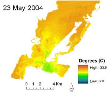
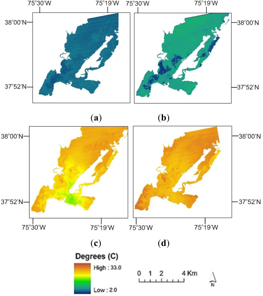
Initial results illustrated in Figure 4 revealed the seasonal trends and pattern of water surface temperatures across a generally north-south gradient from Chincoteague Inlet, through the main channels and around Chincoteague Island into the southern bay. Although covering multiple years, the series shows the predominant seasonal trend of increasing water temperature into summertime and decreasing bay and marine temperature contrast. Two exceptions to this trend are revealed in Figure 4(b), which shows marked cooler temperatures in intertidal marsh and shallows and Figure 4(c), which indicates relatively strong thermal contrast between the flood tide waters and the interior lagoon temperature. Since the image in Figure 4(b) is late May 2004, this season is representative of the onset of more rapid estuarine water heating versus the slower heating of flood tide coastal marine waters. A reversal of this pattern may be expected during the autumn, when the lagoon cools faster than the adjoining ocean arising from the lower volume and loss of heat in the lagoon.
4.2. Flood Tide Repletion Zones
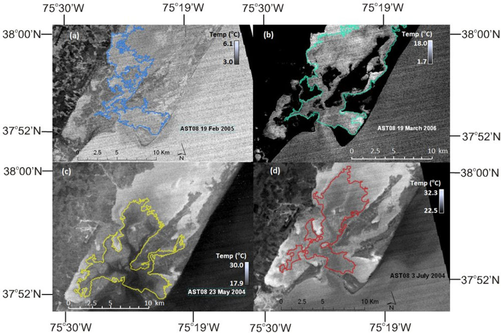
Utilizing the seed pixel homogeneity feature extraction method, each derived flood tide boundary was mapped for visual analysis and comparison (Figure 5). Table 2 summarizes the seed pixel temperature, threshold, and each scene surface water temperature range. Seed pixels were chosen in the throat of Chincoteague Inlet with exclusion of separate internal polygons. Values were iteratively adjusted by increasing the Euclidean threshold until the zone expanded to include the visually discernible extent of the flood tide in the scene. These thresholds are later compared with the distribution of scene temperature ranges, flood repletion zone temperatures, and in situ observations (Table 2 and Figures 6–8.) The flood tide penetrates an average of approximately 10 km from the inlet throat to the distal interior boundary in the lagoon. Subject to estuarine circulation and winds, the bays and intertidal areas closest to the inlet are most well flushed. An exception shown in Figure 5(a) is to the west of the inlet, where only slight penetration is evident as compared with the cove to the east. For all images, the flood tide penetrates 4–5 km or more past the Town of Chincoteague, highlighted as a point symbol in Figure 5. A potential limitation of this discrete delineation is also found in Figure 5(d), which only shows slight tidal penetration into the coves adjoining the inlet. It is likely in these very shallow, clear waters that summer time heating of adjoining surfaces could rapidly heat the incoming tidal waters, even for nighttime images such as these. Given the modest thermal contrast between ocean and lagoonal waters in mid-summer, the tidal water delineation such as Figure 5(d) could be underestimated by this technique. Similarly, low thermal differentiation in the February scene (Figure 5(a)) also lends to less contrast and more potential error. In addition, these two scenes (mid-winter and mid-summer) exhibited the lowest range of temperatures (Table 2.)
4.3. Spatial Zonation and Variation
Prior to evaluating further spatial pattern and variation, the measured water temperatures of flood tide and “residual” lagoonal waters (water mass believed to be resident and not-recirculated in the tidal flushing) were evaluated using exploratory statistics and visual analysis. Figure 6 shows the resulting distributions of residual and flushing tidal waters for each scene, underscoring the prior interpretation of low thermal contrast between coastal and lagoon waters during mid-late winter (February and March scenes, Figure 6(a,b)) and gradually increasing contrast as lagoonal waters more rapidly warmed relative to the ocean by late May (Figure 6(c)). However, one potential discrepancy was revealed in the plot for July 2004 (Figure 6(d)), which exhibited a greater degree of contrast between the tidal and residual water in the lagoon. Since these plots portray the distribution for all image pixels, it can be inferred that this likely masks the fact that some flushing tidal waters could rapidly warm in extreme shallows and amidst warm air advection in this breezy coastal location. Thus, it is likely that there exists a combination of mixing and shallow tidal water heating that confuses the higher temperature residual water mass with mixed and rapidly-warmed tidal influx. Comparison of results to circulation or detailed in situ measurements would be necessary to further affirm this interpretation.
4.3.1. Verification with in situ Observations
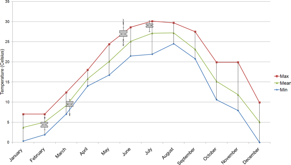
Although simultaneous “sea truth” observations were unavailable for validation, the ASTER temperature images compared well to the in situ observations recorded in the long-term State of Maryland “Eyes on the Bay” monitoring program (Figure 7). The line plot in this figure shows the distribution of the repletion waters to fall within the range and close to the monthly mean temperatures for Chincoteague during the months observed. The Eyes on the Bay station (#XBM1301) is in the middle of Chincoteague Bay astride the Virginia-Maryland border but just north of the typical interior boundary of flood tide waters. The ASTER scene residual water temperature estimates are typically below the average in February and March and within the range of in situ observations for May and July, corroborating the capability of ASTER TIR data to capture seasonal estuarine water temperature trends and infer patterns for individual dates and scenes. These differences may be explained by the individual conditions of the scenes observed and associated mixing. The scene-averaged residual water temperature is also restricted to the subset areas of ASTER scenes analyzed. This does not encompass the entirety of the lagoon and particularly the interior, less flushed and likely colder waters on the Maryland portion of the bay.
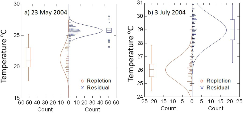
In addition to the box plots, water mass temperature distributions show overlap but distinct differences in means and variance between flood tide and residual waters (Figure 8). The flood repletion waters comprised a wider range of temperatures and overlapped the residual water temperatures at the cool range, while the residual lagoon waters were more homogeneous and warmer overall (Figure 8(a)) in May. As the summer season progressed and insolation and warm air advection increase the temperature of both the lagoon and coastal ocean, the evident difference diminishes (Figure 8(b)) and the range of overlap increases. These observations affirm the spatial patterns of temperature and highlight the increasing difficulty discerning a discrete tidal repletion boundary via thermal data in mid-summer. Nonetheless, the overall mean and range of ASTER-derived residual lagoon water temperatures and their seasonal temperature trends of the lagoon are corroborated by the Eyes on the Bay data.
4.3.2 Zonation and Principal Components Analysis
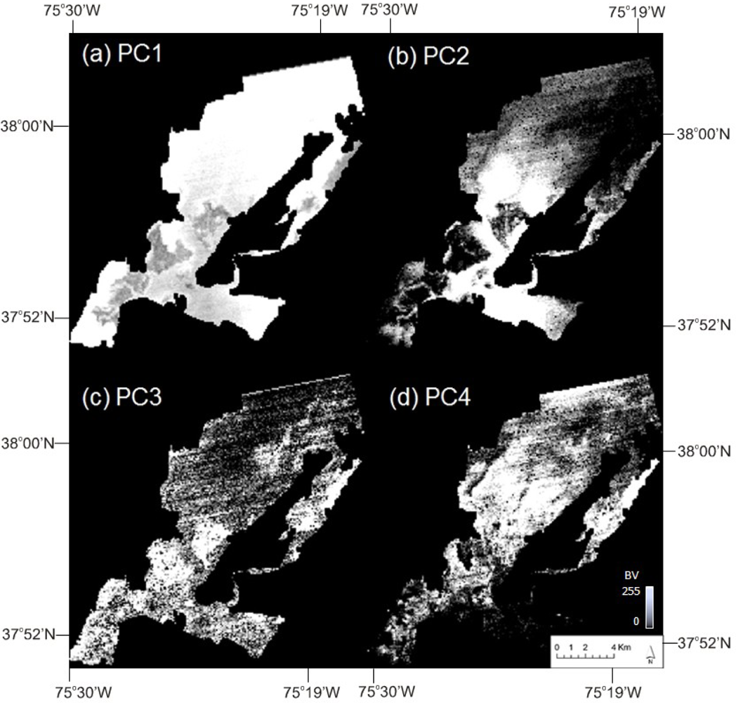
Results from PCA analysis are shown in tabular and graphical image form in Table 3 and Figure 9, respectively. The resulting eigenvalues illustrate that the first principal component (PC 1) summarizes nearly 96% of the input variance in the four thermal scenes investigated. The associated eigenvectors load nearly equally on the input images and also strongly highlight the zone of residual lagoonal water (Figure 9(a)). PC 1 is interpreted to capture the prevailing zone of residual water, indicating a broader area of homogeneity among the images. PC 2, in contrast, captures only approximately three percent (0.028 proportion of input variance) yet loads differentially, negatively in the cool months (February and March) versus positively in the warm months (May and July). The corresponding PC 2 image also markedly contrasts a zone corresponding to the generalized flood tide, shown as light tone (Figure 9(b)) This PC 2 image is thus interpreted to capture the average flood tide. Results from PC 3 and 4 captured less input variance, only approximately one percent (PC 3) and one-half percent (PC 4), respectively. The weighting is also more idiosyncratic, with PC 3 loading mainly on the February scene, and PC 4 mainly on the May temperature image. The spatial pattern of PC 3, however, is suggestive of the effects of intertidal marshes, which could advect heat loss to the atmosphere more readily. This area (Figure 9(c)) shows as a light tone and correlates to the February and March “cool spot” phenomena previously observed in Figure 4(a,b). The image for PC4 (Figure 9(d)) contains less overall contrast and subtle artifacts of scanline noise and bias in the sensor. Nonetheless, there is a spatial gradient of contrast that focuses on a repletion zone of mixing, mid-way through the flood tide plume. This inferred PC4 “zone of mixing” captures temporal-spatial variation of tidal flooding less well conveyed in the discrete feature extraction approach found in Figure 5.
4.4. Discussion
Results of this investigation reveal strong potential for satellite data such as ASTER TIR response to delineate tidal flooding and repletion in coastal lagoons and estuaries. Synoptic assessments of tidal flushing patterns can improve water level zoning and hydrographic surveying for the siting of tide stations and correction algorithms for bathymetry. However, there is room for improvement in the delineation of discrete tidal flushing zones, such as better integration of astronomical and harmonic components in hydrodynamic models and networks of water level and water quality monitoring. Overall, this investigation provides a foundation of first-order estimates using thermal satellite earth observation to predict hydraulic turn-over in lagoons and estuaries for managers seeking more information on watershed, estuary, and eutrophication vulnerability assessment. Subsequent investigations might explore composite repletion footprints to estimate tidal volume and hydraulic turn-over time, including other tidal stages, extreme events, or tidal progression with stereo observations. A longer time series of thermal satellite data might also be able to develop a coastal or estuarine sea surface temperature climatology and fine-scale data on surface energy fluxes, which would benefit ecological monitoring and management. The relatively high-resolution of ASTER TIR data shown here has evident potential for extensive and numerous coastal lagoons and bays with inlets and tidal creek channels. A longer time series of surface temperatures over such waters could also provide information on energy fluxes and micrometeorological processes that might improve forecasting (e.g., sea breezes and wind power) as compared with coarser satellite data. Observed tidal flushing from satellite also holds value in for assessing the range of uncertainty and variability of tidal repletion volumes under different meteorological forcing, particularly in small and/or distant coastal bays and lagoons where model data are limited and in situ observations expensive or infeasible. Management applications of these data include coastal ecological monitoring and restoration, such as seagrass restoration, benthic habitat assessment such as oysters, clam and aquaculture uses, and water quality protection. The availability of repetitive satellite thermal imagery and the synoptic approach presented thus provides an efficient means for resource monitoring as well as scientific investigation of estuarine processes.
The availability of TIR data on Landsat-7 ETM+ sensor with 60 m spatial resolution and sensitivity to 10.4–12.5 mm has not been overlooked in this study and remains highly applicable. Even with the onset of the Scan-Line Corrector (SLC) anomaly, Landsat-7 continued to collect data, which has since been provided free as well as reliably with interpolation and SLC-off post-processing [23,24]. However, preliminary searches on the Landsat-7 archive discovered frequent obscuration of data collected during daytime observing and a paucity of imagery available during appropriate near flood-tide conditions in the relatively short timespan focused upon by this study. Other studies have applied Landsat-7 TIR data successfully to regional oceanographic sea-surface temperature over longer timespans [12,13] or in relatively more arid environments than the coastal investigation herein [14,15]. Nonetheless, Landsat TIR data have a long history and near-global data availability, providing for possible historical change analysis or systematic coastal lagoon comparative research. In addition, the Landsat Data Continuity Mission (LDCM), scheduled to launch in 2013, will contain a Thermal Infrared Sensor (TIRS) package sensitive in two longwave bands (10.3–11.3 mm and 11.5–12.5 mm) with 100 m resolution, 12-bit data depth, and improved signal-to-noise ratio [25].
5. Conclusions
Our study results affirmed the feasibility and efficacy of ASTER TIR satellite data for analysis of tidal repletion patterns surrounding Chincoteague Inlet, Virginia, over a range of seasonal contrasts between ocean sea surface and lagoonal temperatures. Further scientific analysis could benefit from integration of such remote sensing with hydrodynamic modeling and coastal geospatial analysis of diverse estuarine processes and resource assessments. Satellite TIR imagery could also be useful to assess variability and anomalous meteorological forcing, such as lagoonal conditions during droughts, floods, or pre-/post-storm events. Specific insights from this project offer suggestions for subsequent research. First, search and discovery of ASTER Quicklook imagery in conjunction with tidal data proved valuable and efficient for selecting the most appropriate and highest data quality of imagery. The availability of Quicklook imagery and metadata is thus an important asset to the initial phases of this research. Second, algorithms for TIR data normalization and conversion to skin surface temperature were corroborated against in situ observations. However, as in situ data are often sparsely available, future studies should secure this availability in advance, ideally having access to a cross-section or spatial sampling that would coincide with residual, mixing, and inlet zones such as structured in this study. While meteorological data were not rigorously analyzed in this investigation, access to a numerical hydrodynamic simulation model would potentially improve the analysis and explain the typicality or atypicality of the zones delineated in our temporal analysis. Although numerical models require their own significant data inputs, the products of flushing time, residence time and circulation patterns would add to the inferences as well as provide model calibration. Nonetheless, numerical models which remain relatively rare in small coastal bays in lagoons, so this study has demonstrated the feasibility of mapping zones of mixing and repletion with a straightforward image processing methodology. The use of seed-pixel thresholding performed well for flood tide waters delineation, with the ensuing repletion waters matching closely to the in situ water observation data. PCA analysis also highlighted the variability of the zonation.
Having demonstrated ASTER multitemporal thermal data for analysis of tidal repletion, flushing, and flood tidal waters, a variety of other investigations are deemed feasible. Since many coastal bays and lagoons are interconnected along trailing continental margins with barrier islands, satellite TIR data could be useful to investigate inter-lagoonal water volume exchanges, upwelling, fronts, and plumes. High-resolution satellite TIR data may also further exploit the degree of mixing and quantitative estimation of “benthic weather” such as affects lagoon habitats, flora, fauna, and aquaculture, which optical multispectral remote sensing cannot discern, particularly in frequently turbid coastal environments. Future understanding of these phenomenon and management of coastal resources will be enhanced with the continued availability of thermal satellite imagery such as planned for the NASA Landsat Data Continuity Mission.
Acknowledgments
The author appreciates the support and facilities provided by the Center for Geographic Information Science and Renaissance Computing Institute (RENCI) at East Carolina University. George F. Oertel and George McLeod of Department of Ocean, Earth, and Atmospheric Sciences (OEAS), Old Dominion University, provided supporting literature and background on tidal hydraulics for the study. Two anonymous reviewers provided substantial suggestions to improve the manuscript.
References
- Kjerfve, B.J.; Magill, K.E. Geographic and hydrodynamic characteristics of a shallow coastal lagoon. Mar. Geology 1989, 88, 187–199. [Google Scholar]
- Boone, J.D.; Byrne, R.J. On basin hypsometry and morphodynamic response of coastal inlet systems. Mar. Geology 1981, 40, 27–48. [Google Scholar]
- Eiser, W.C.; Kjerfve, B.J. Marsh topography and hypsometric characteristics of a shallow coastal lagoon. Mar. Geology 1986, 88, 187–199. [Google Scholar]
- Oertel, G.F. Hypsographic, hydro-hypsographic and hydrological analysis of coastal bay environments, Great Machipongo Bay, Virginia. J. Coastal Res 2001, 17, 775–783. [Google Scholar]
- Oertel, G.F.; Overman, K.; Carlson, R.; Porter, J.H.; Allen, T.R. Hypsographic Analysis of Coastal Bay Environments Using Integrated Remote Sensing Techniques, Great Machipongo Bay, Virginia. Proceedings of 6th International Conference Remote Sensing for Marine and Coastal Environments, Charleston, SC, USA, 1–3 May 2001; pp. 269–276.
- Takeoka, H. Fundamental concepts of exchange and transport time scales in a coastal sea. Cont. Shelf Res 1984, 3, 311–326. [Google Scholar]
- Matthews, J. Stereo observation of lakes and coastal zones using ASTER imagery. Remote Sens. Environ 2005, 99, 16–30. [Google Scholar]
- Ferrier, G.; Macklin, J.T.; Neill, S.P.; Folkard, A.M.; Copeland, G.J.M.; Anderson, J.M. Observing estuarine currents and fronts in the Tay Estuary, Scotland, using an airborne SAR with Along-Track Interferometry (ATI). Int. J. Rem. Sens 2005, 26, 4399–4404. [Google Scholar]
- Gillespie, A.; Rokugawa, S.; Matsunaga, T.; Cothern, J.S.; Hook, S.; Kahle, A.B. A temperature and emissivity separation algorithm for advanced spaceborne thermal emission and reflection radiometer (ASTER) images. IEEE Trans. Geosci. Remote Sens 1998, 36, 1113–1126. [Google Scholar]
- Trunk, L.; Bernard, C.A. Investigating crater lake warming using ASTER thermal imagery: Case studies at Ruapehu, Poás, Kawah Ijen, and CopahuéVolcanoes. J. Volcanol. Geothermal Res 2008, 178, 259–270. [Google Scholar]
- Dinnel, S.P.; Schroeder, W.W.; Wiseman, W.J., Jr. Estuarine-shelf exchange using Landsat images of discharge plumes. J. Coastal Res 1990, 6, 789–799. [Google Scholar]
- Thomas, A.; Byrne, D.; Weatherbee, R. Coastal sea surface temperature variability from Landsat infrared data. Remote Sens. Environ 2002, 81, 262–272. [Google Scholar]
- Fisher, J.I.; Mustard, J.F. High spatial resolution sea surface climatology from Landsat thermal infrared data. Remote Sens. Environ 2004, 90, 293–307. [Google Scholar]
- Handcock, R.N.; Gillespie, A.R.; Cherkauer, K.A.; Kay, J.E.; Burges, S.J.; Kampf, S.K. Accuracy and uncertainty of thermal-infrared remote sensing of stream temperatures at multiple spatial scales. Remote Sens. Environ 2006, 100, 427–440. [Google Scholar]
- Laymon, C.A.; Quattrochi, D.A. Estimating Spatially Distributed Surface Fluxes in a Semi-Arid Great Basin Desert Using Landsat TM Thermal Data. In Thermal Remote Sensing in Land Surface Processes; Quattrochi, D.A., Luval, J.C., Eds.; CRC Press: Boca Raton, FL, USA, 2004; pp. 133–159. [Google Scholar]
- Miliaresis, G.; Partsinevelos, P. Terrain segmentation of Egypt from multi-temporal night LST imagery and elevation data. Remote Sens 2010, 2, 2083–2096. [Google Scholar]
- Environmental Protection Agency (EPA), Delmarva’s Coastal Bay Watersheds: Not up the Creek Yet; Report R-96/052; EPA Office of Research and Development, US EPA: Ocean City, MD, USA, 1996.
- Wazniak, C.; Hall, M.; Cain, C.; Wilson, D.; Jesien, R.; Thomas, J.; Carruthers, C.; Dennison, W. State of the Maryland Coastal Bays. 2004. Available online: http://www.mdcoastalbays.org/archive/2004/MCB-State-Bay-2004.pdf (accessed on 17 August 2005).
- Bricker, S.B.; Clement, C.G.; Pirhalla, D.E.; Orlando, S.P.; Farrow, D.R.G. National Estuarine Eutrophication Assessment: Effects of Nutrient Enrichment in the Nation’s Estuaries; National Ocean Service, Special Projects Office and the National Centers for Coastal Ocean Science: Silver Spring, MD, USA, 1999. [Google Scholar]
- Bricker, S.B.; Longstaff, B.; Dennison, W.; Jones, A.; Boicourt, K.; Wicks, C.; Woerner, J. Effects of Nutrient Enrichment in the Nation’s Estuaries: A Decade of Change (National Estuarine Eutrophication Update); National Ocean Service, National Centers for Coastal Ocean Science: Silver Spring, MD, USA, 2007. [Google Scholar]
- National Aeronautics and Space Administration, ASTER Higher-Level Product User Guide, Version 2.0; Report JPL D-20062; NASA Jet Propulsion Laboratory, California Institute of Technology: Pasadena, CA, USA, 2001; p. 80.
- Hook, S.J.; Myers, J.J.; Thome, K.J.; Fitzgerald, M.; Kahle, M.B. The MODIS/ASTER airborne simulator (MASTER)—A new instrument for earth science studies. Remote Sens. Environ 2001, 76, 93–102. [Google Scholar]
- Jimenez-Munoz, J.C.; Sobrino, J.A. Feasibility of retrieving land-surface temperature from ASTER TIR bands using two-channel algorithms: A case study of agricultural areas. IEEE Geosci. Remote Sens. Lett 2007, 4, 460–464. [Google Scholar]
- NASA. Landsat 7 Science Data Users Handbook. Available online: http://landsathandbook.gsfc.nasa.gov/pdfs/Landsat7_Handbook.pdf (accessed on 14 September 2012).
- NASA. Landsat Data Continuity Mission (LDCM). Available online: http://www.nasa.gov/mission_pages/landsat/spacecraft/index.html (accessed on 14 September 2012).
Figure 1.
Study area southern Chincoteague Bay and Chincoteague Inlet, Virginia.

Figure 2.
Selected ASTER Quicklooks for band 13 thermal images (60 km swath) used for selection and tidal stage analysis. Location of Chincoteague Inlet highlighted (★). Image acquisition and nearest high tide (HW) at Chincoteague Inlet Local Standard Time (LST) (a) 23 May 2004, (b) 3 July 2004, (c) 21 September 2004, and (d) 17 December 2004.

Figure 3.
ASTER time series for band 13 thermal Quicklook images (60 km swath) used for image selection and tidal stage analysis. Location of Chincoteague Inlet highlighted (★). Time of image acquisition and nearest low water (LW) tide or high tide (HW) at Chincoteague Inlet in Local Standard Time (LST) (a) 19 February 2005, (b) 7 March 2005, (c) 17 April 2005, and (d) 10 May 2005.
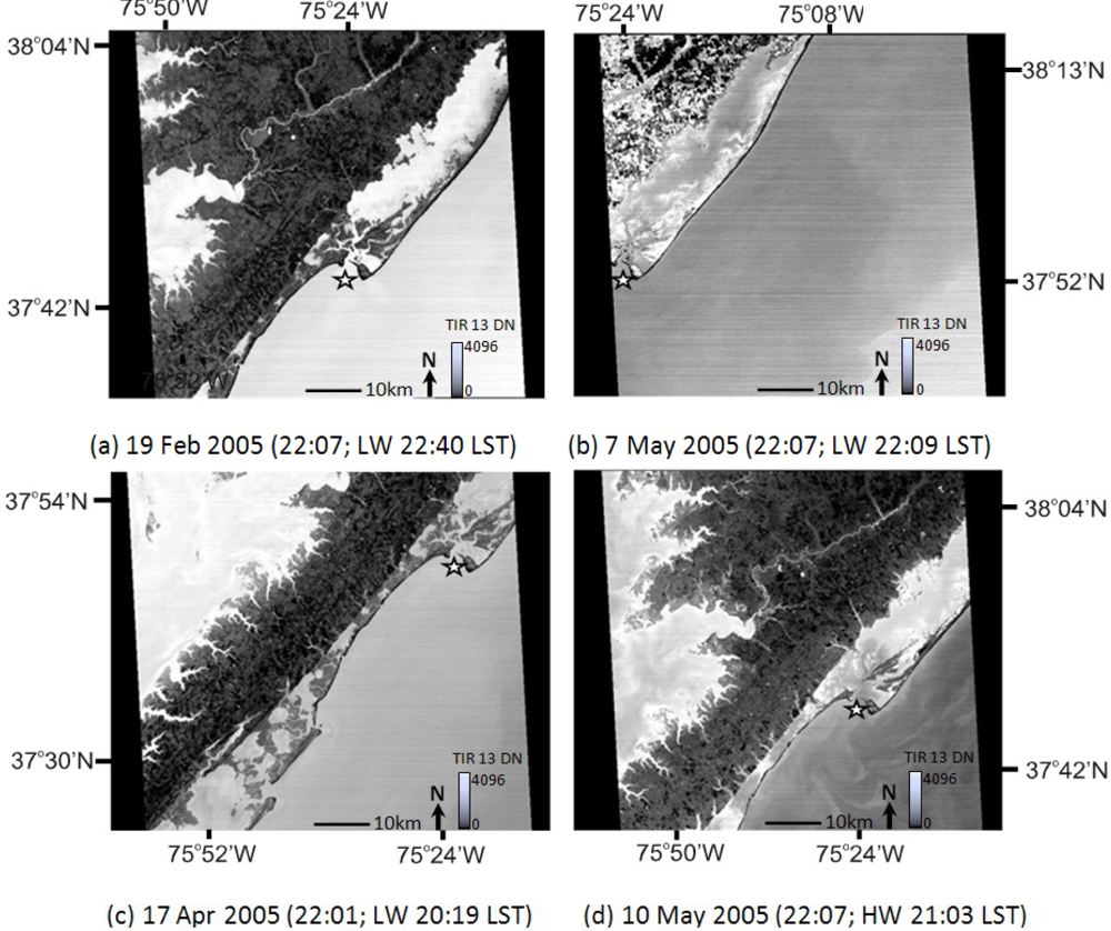
Figure 4.
ASTER time series surface temperature for water surfaces masked from land and transformed to skin surface temperature (a) 19 February 2005, (b) 19 March 2006, (c) 23 May 2004, and (d) 3 July 2004.
Figure 4.
ASTER time series surface temperature for water surfaces masked from land and transformed to skin surface temperature (a) 19 February 2005, (b) 19 March 2006, (c) 23 May 2004, and (d) 3 July 2004.

Figure 5.
Derived surface water temperatures and repletion footprints for each image highlighting the Town of Chincoteague (★) for location reference (a) 19 February 2005, (b) 19 March 2006, (c) 23 May 2004, and (d) 3 July 2004.
Figure 5.
Derived surface water temperatures and repletion footprints for each image highlighting the Town of Chincoteague (★) for location reference (a) 19 February 2005, (b) 19 March 2006, (c) 23 May 2004, and (d) 3 July 2004.

Figure 6.
Box plots of ASTER-derived skin surface temperatures for flood repletion and residual lagoon water bodies (a) 19 February 2005, (b) 19 March 2006, (c) 23 May 2004, and (d) 3 July 2004.
Figure 6.
Box plots of ASTER-derived skin surface temperatures for flood repletion and residual lagoon water bodies (a) 19 February 2005, (b) 19 March 2006, (c) 23 May 2004, and (d) 3 July 2004.
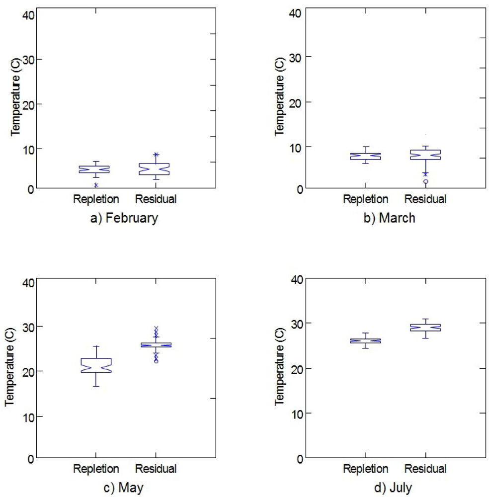
Figure 7.
Box plots of ASTER-derived skin surface temperatures for flood repletion water mass (box plots) with line plots of in situ mean, minimum, and maximum monthly 2001–2011 water temperatures for Chincoteague (Maryland Department of Natural Resources, “Eyes on the Bay” http://mddnr.chesapeakebay.net/eyesonthebay/ [18]).

Figure 8.
Frequency distributions and boxplots of derived ASTER skin surface flood tide repletion and residual lagoon water mass temperatures for sampled pixels (a) May and (b) July 2004 images.
Figure 8.
Frequency distributions and boxplots of derived ASTER skin surface flood tide repletion and residual lagoon water mass temperatures for sampled pixels (a) May and (b) July 2004 images.

Figure 9.
PCA brightness value images on normalized 8-bit range derived from time series ASTER temperature images (a) PC 1, (b) PC 2, (c) PC 3, and (d) PC 4.
Figure 9.
PCA brightness value images on normalized 8-bit range derived from time series ASTER temperature images (a) PC 1, (b) PC 2, (c) PC 3, and (d) PC 4.


Table 1.
Selected image acquisition times, flood/ebb peaks, and tidal offsets (Local Standard Time).
| Image Date | Image Acquisition (LST) | Tide (LST) | Image-Tidal Stage Offset (min) | Note |
|---|---|---|---|---|
| 19 February 2005 | 22:07 | Low 22:40 | −33.0 | Nearest mean low water (MLW) |
| 19 March 2006 | 22:01 | High 22:27 | −26.0 | Near high water |
| 23 May 2004 | 22:08 | High 23:16 | −68.0 | Near high water |
| 3 July 2004 | 22:01 | High 22:07 | −6.0 | Nearest mean high water (MHW) |
Table 2.
Seed pixel temperature, threshold, and water surface temperatures in tide feature extraction.
| Image Date | Seed Pixel Temperature (°C) | Euclidean Threshold (°C) | Scene Temperature Range (°C) |
|---|---|---|---|
| 19 February 2005 | 6.0 | ±0.5 | 3.3–6.1 |
| 19 March 2006 | 5.0 | ± 1.0 | 1.7–17.8 |
| 23 May 2004 | 18.9 | ± 2.5 | 17.9–30.0 |
| 3 July 2004 | 24.5 | ± 1.5 | 22.5–32.3 |
Table 3.
Eigenvalues and eigenvectors for time series Principal components analysis (PCA) for differentiation of water masses.
| Principal Components | ||||
| 1 | 2 | 3 | 4 | |
| Eigenvalues (variance proportion) | 15,139.80 (0.958) | 438.707 (0.028) | 131.679 (0.008) | 85.652 (0.005) |
| Eigenvectors | ||||
| 19 February 2005 | 0.419 | 0.419 | 0.804 | 0.022 |
| 19 March 2006 | 0.641 | 0.490 | −0.589 | −0.032 |
| 23 May 2004 | 0.469 | −0.544 | 0.019 | 0.694 |
| 3 July 2004 | 0.438 | −0.535 | 0.070 | −0.718 |
Share and Cite
MDPI and ACS Style
Allen, T.R. Estimating Coastal Lagoon Tidal Flooding and Repletion with Multidate ASTER Thermal Imagery. Remote Sens. 2012, 4, 3110-3126. https://doi.org/10.3390/rs4103110
AMA Style
Allen TR. Estimating Coastal Lagoon Tidal Flooding and Repletion with Multidate ASTER Thermal Imagery. Remote Sensing. 2012; 4(10):3110-3126. https://doi.org/10.3390/rs4103110
Chicago/Turabian StyleAllen, Thomas R. 2012. "Estimating Coastal Lagoon Tidal Flooding and Repletion with Multidate ASTER Thermal Imagery" Remote Sensing 4, no. 10: 3110-3126. https://doi.org/10.3390/rs4103110