Decision Tree and Texture Analysis for Mapping Debris-Covered Glaciers in the Kangchenjunga Area, Eastern Himalaya

1
Department of Geography and Institute of Arctic and Alpine Research, University of Colorado, CB 450, Boulder, CO 80303, USA
2
Laboratoire de Glaciologie et Géophysique de l’Environnement, 54 rue Molière, Domaine Universitaire, BP 96, Saint Martin d’Hères cedex 38402, France
*
Author to whom correspondence should be addressed.
Remote Sens. 2012, 4(10), 3078-3109; https://doi.org/10.3390/rs4103078
Submission received: 16 August 2012
/
Revised: 26 September 2012
/
Accepted: 29 September 2012
/
Published: 18 October 2012
(This article belongs to the Special Issue Earth Observation Technology Cluster: Innovative Sensor Systems for Advanced Land Surface Studies)
Abstract
:In this study we use visible, short-wave infrared and thermal Advanced Spaceborne Thermal Emission and Reflection Radiometer (ASTER) data validated with high-resolution Quickbird (QB) and Worldview2 (WV2) for mapping debris cover in the eastern Himalaya using two independent approaches: (a) a decision tree algorithm, and (b) texture analysis. The decision tree algorithm was based on multi-spectral and topographic variables, such as band ratios, surface reflectance, kinetic temperature from ASTER bands 10 and 12, slope angle, and elevation. The decision tree algorithm resulted in 64 km2 classified as debris-covered ice, which represents 11% of the glacierized area. Overall, for ten glacier tongues in the Kangchenjunga area, there was an area difference of 16.2 km2 (25%) between the ASTER and the QB areas, with mapping errors mainly due to clouds and shadows. Texture analysis techniques included co-occurrence measures, geostatistics and filtering in spatial/frequency domain. Debris cover had the highest variance of all terrain classes, highest entropy and lowest homogeneity compared to the other classes, for example a mean variance of 15.27 compared to 0 for clouds and 0.06 for clean ice. Results of the texture image for debris-covered areas were comparable with those from the decision tree algorithm, with 8% area difference between the two techniques.
1. Introduction
High-relief glacierized mountain ranges such as the Himalaya, the Karakoram and Alaska are characterized by the presence of heavy debris in the ablation areas of glacier tongues [1–3]. This limits field observations and prevents the full understanding of the dynamics of these glaciers, and their response to climatic changes. Debris material in these areas originates by rockfall from the steep valley sides, and is incorporated onto the glacier ice, building a continuous supraglacial debris mantle in the ablation zone of glaciers. These debris-covered tongues are typically characterized by alternating ridges and depressions on the order of 20–50 m in height, exposed ice cliff walls and supraglacial lakes [4,5]. Such features pose practical difficulties for glacier monitoring; hence field-based surveys are generally scarce, particularly in high Asia [4,6–11]. Given the concern for the growth of pro-glacier lakes, the potential for glacier lake outburst floods and the role of debris-covered glaciers in regional hydrology [12,13], there is currently high interest in understanding the behavior of these glaciers at larger spatial scales. Accurate estimates of debris cover area, thickness and thermal properties are needed to determine melting rates over these glacier tongues, and are increasingly addressed in glaciologic studies [10,11,14,15].
Debris cover is of interest to glaciologists due to its influence on the glacier melt processes. A thick debris cover (> a few centimeters, or “critical thickness”) has been shown to reduce the ablation rates of the ice underneath due to the low thermal conductivity of debris [10,14,16], whereas a thin debris cover (< a few centimeters) was shown to increase the ice melt rates due to the low albedo of the debris [17–19]. The critical thickness is defined as the thickness at which the sub-debris ice melt rate equals the clean ice melt rate at a particular location. However, ice continues to melt at a low rate for debris thicknesses even beyond this critical thickness [10,16]. Understanding the various controls on glacier melt processes on these debris-covered tongues is complicated and not fully understood in areas such as the Himalaya (in particular the role of ice cliff walls and supraglacial lakes) [20]. Several studies reported rates of thinning of debris-covered tongues comparable to those of clean ice [21–25], with a low ice flux to glacier tongues. Other studies from the Karakoram and the Alps [26–29], in contrast, reported a thickening of these glacier tongues due to either mass gain or glacier surges. Despite recent progress on characterizing the surface topography and thickness of debris cover [4,14,30], detailed information is still needed to characterize debris-covered glaciers at large scales in areas such as the Himalaya, perhaps using satellite data [20].
Previous remote sensing studies have established that mapping of debris-covered glaciers using multi-spectral information alone is challenging [31–34]. Therefore, in the last decade, a number of studies focused on combining multispectral and topographic information to delineate debris-covered glaciers. Among these approaches we mention: (1) a semi-automated approach based on a slope map, a false color composite of Landsat TM bands 3–5 and TM 4/TM 5 band ratio [35]; (2) morphologic approaches using clusters of curvature features [36] and (3) a hierarchical approach based on slope, elevation, aspect and terrain curvature [37]. These mapping methods are all considered “semi-automated” because they all involve manual digitization to some degree [38,39]. An increasing number of studies rely on the thermal capability of ASTER data for mapping the extent, thickness and thermal characteristics of debris-covered ice. Such approaches have been tested in the last decade for individual glaciers in the Himalaya [11,14,32,33,40–43] and the Alps [10,15,16,26,44]. A recent study [6] used visible to thermal infrared multi and hyperspectral analysis to characterize the geologic composition of glacier debris at a regional scale (Khumbu Himalaya, Nepal). Another study [45] proved the potential of ASTER thermal imaging for discriminating debris-covered and rock-covered glaciers using night-time and day-time images. Thermal mapping approaches rely on the cooling effect of the ice on the supraglacial debris. Supraglacial debris cover is generally several degrees colder than lateral moraines [15], except for areas where the debris cover is thick and continuous (hence insulated), or when the surrounding moraines are in shadow (hence colder than supraglacial debris) [33,46].
A major limitation for mapping debris-covered glaciers at large scales using the synergistic approaches mentioned above (multispectral and topographic data) is due to the heterogeneous distribution of the debris cover thickness and thermal properties along these glacier tongues. In this study we suggest that texture analysis may provide alternate methods for capturing spatial distribution of debris cover properties. Although used in textile inspection or medical image processing [47] and land cover classification (such as types of agricultural crops or urban analysis) [48], texture analysis has been only sparsely applied to debris-covered glaciers, for example for surface feature detection on synthetic aperture radar (SAR) images [49–52]. To our knowledge, however, texture measures using optical remote sensing have not been tested for mapping debris cover in the Himalayas.
In a previous paper [53], we presented an overview of a decision tree algorithm based on topographic and multi-spectral measures for mapping potentially debris-covered ice in the eastern Himalaya. Here we fully describe this method, and expand on the potential of ASTER surface temperature data and texture analysis for mapping the debris cover characteristics. We use high-resolution imagery from Quickbird (QB) and WorldView2 (WV2) for validating our results. We visually compare the output of the decision-tree algorithm with manually-digitized debris cover outlines based on texture analysis, as a basis for a future approach to debris cover mapping.
2. Study Area
Sikkim Himalaya (27°04′52″N to 28°08′26″N latitude and 88°00′57″E to 88°55′50″E longitude) is located in eastern India, between Nepal and Bhutan (Figure 1). This part of the Himalaya is situated under the monsoon influence characterized by “summer-accumulation type” glaciers, where accumulation and ablation occur concomitantly in the summer [54]. The study area also includes glaciers at the border with China (Tibetan plateau), and the Kangchenjunga glaciers in eastern Nepal. Relief ranges from 300 m at lowlands to 8,598 m (the summit of Mt. Kangchenjunga), with steep and rugged topography. There were 449 glaciers covering an area of 705.54 km2 in Sikkim during the 1970s, based on an inventory constructed from 1970 topographic maps [55]. Mool et al. [13] reported 285 glaciers covering an area of 576.4 km2 on the basis of 2000 Landsat ETM+ imagery. For testing of the debris cover algorithms and the texture analysis, we focus on ten glaciers, including Yalung, Onglaktang and Zemu glacier, all shown in Figure 1. Zemu is one of the longest valley-type glaciers in the Himalayas (∼26 km), and is the headwaters of the Tista River, which provides important water resources to lowlands [13]. We surveyed the area around Onglaktang glacier in western Sikkim in November 2006, acquiring photographs of the debris-covered tongue and the lateral moraines (Figure 2).
3. Data Sources and Methodology
3.1. Data Sources
A topographic map at 1:150,000 scale was used to infer the approximate location of debris-covered tongues in this area (Figure 3). The map was compiled from Survey of India maps dating from the 1960s–1970s and was published by the Swiss Foundation for Alpine Research. The exact date of each quadrant is not available because of restrictions on Indian topographic data [56,57]; therefore, we assume this map to date from the 1960s–1970s. Debris-covered tongues were delineated manually using on-screen digitization from the map and were split into individual glaciers using topographic information from the void-free and hydrologically-sound Shuttle Radar Topography Mission (SRTM) DEM, provided by CGIAR [58] and the ice divide protocol developed by [59].
An ASTER scene acquired on 27 November 2001 (04:57 UTC, 10:27 a.m. local time) was chosen as the main data source for this study based on minimal cloud cover, good contrast over snow and ice, and suitable date of acquisition (end of the ablation season) (Figure 1). The scene was almost cloud-free over the glaciers except some clouds in the southern part of the image; there was some transient snow on the glaciers and surrounding bare land (Figure 1). Two products were obtained from the EROS Data Center ( http://eros.usgs.gov/): AST14DMO (the orthorectified product package based on registered radiance at sensor L1B) and AST08 (the surface kinetic temperature). The orthorectified AST14DMO product consists of the 14 ASTER bands and a DEM constructed on-demand at LPDAAC from bands 3n and 3b using Silcast software, with no ground control points. The accuracy of the ASTER DEMs is reported to be less than 25 m (root mean square error in the vertical coordinate, RMSEz) [60].
Two QB scenes acquired in January 2006 were ordered from Digital Globe as ortho-ready standard imagery. These are radiometrically-calibrated scenes, corrected for sensor and platform distortions [61]. The scenes were orthorectified using the SRTM DEM CGIAR version and mosaicked in ERDAS Imagine Leica Photogrammetry Suite (LPS). The nominal pixel size for QB images was 2.4 m; we resampled these to 3 m-pixel size during the orhorectification process using a cubic convolution method. These scenes cover an area of 1,107 km2 and were well contrasted and snow-free. A WV2 scene acquired on in December 2010 was used to map the terminus of Zemu glacier, which was missing from the QB image. The WV2 scenes are panchromatic, ortho-ready scenes with a spatial resolution of 50 cm. We used the QB and WV2 scenes to digitize debris-covered tongues manually, using on-screen digitizing on a using a color composite (QB 321) and panchromatic (WV2 imagery). These glacier outlines were used as validation of the debris-cover output from the ASTER algorithm, on a glacier-by-glacier basis. Characteristics of the remote sensing and topographic data used in this study are summarized in Table 1 below. All datasets were registered to UTM projection zone 45N, with elevations referenced to WGS84 datum. The infrared ASTER bands and the DEM were resampled to 15 m to match the spatial resolution of the visible bands.
3.2. Topographic and Multi-Spectral Analysis
We used ASTER multispectral data (visible near infrared–VNIR, shortwave infrared–SWIR and thermal infrared–TIR) in conjunction with topographic data extracted from the ASTER DEM to develop criteria for potential areas of debris-covered ice, based on previous mapping approaches [31,32,44]. The following criteria were used to exclude types of surfaces unsuitable for the presence of debris, in the following order: clean ice; clouds; vegetated areas; steep slopes; deep shadows; bare rock and sand; elevation and temperature. Clean ice was delineated using band ratio algorithms: the Normalized Difference Snow Index (NDSI) [62,63], and ASTER band 3/4 and 3/5 ratios [38,64]. Band ratios rely on the high reflectivity of ice in the visible bands compared to the low reflectivity in the SWIR bands. Clouds were mapped by thresholding of ASTER band 4, where clouds are more reflective than snow and ice. Vegetation was mapped using the Normalized Difference Vegetation Index (NDVI) method with ASTER bands 3 (NIR) and 2 (Red). The NDVI method is based on the high reflectivity of vegetation in the NIR and high absorbency in the visible bands (red and blue) wavelengths due to the presence of chlorophyll [65]. Steep slopes (>12°–24°) were found unsuitable for the occurrence of debris in previous studies [31,32], so we used a similar approach here. Deep shadows were mapped by thresholding of ASTER band 3, where shadows have low reflectance values. The hue saturation value (HSV) transform was used previously by Paul et al. [31] to map vegetated/non-vegetated areas. Here we used the HSV approach to exclude bare rock and sand from the map of debris-covered areas. An elevation threshold was applied to the ASTER DEM to map areas situated between the regional minimum elevation of the glacier termini and the regional equilibrium line altitude (ELA), where generally most debris-covered ice is situated. We also used the surface temperature product AST08 to investigate the thermal characteristics of the debris cover on the tongue of Zemu glacier. In the final step, the temperature thresholds were determined from thresholding individual ASTER TIR bands.
The thresholds for each criterion were selected quantitatively using statistics of the output images for each criterion. For each output of the criteria above, we drew transects across the surface mapped (i.e., snow/ice, clouds, etc.), and examined the frequency histograms of digital numbers (DN) along transects (the spectral signature in the output image). We also drew regions of interest (ROIs) on the each class mapped, and extracted basic statistics (minimum, maximum and median values). We used these transects and the ROI statistics to choose the thresholds for each class (these are described in detail in Section 4.3). We used a decision tree classifier in ENVI, which performs multistage classifications by using a series of binary decisions to assign pixels in an image into classes. Each condition divided pixels into two classes based on a conditional expression with a threshold, resulting in a binary image. The criteria were then combined to produce a map of potential areas for the occurrence of debris cover on glacier tongues.
3.3. Texture Measures
We selected a subset of the ASTER image (centered on Zemu glaciers in the Kangchenjunga area), sized to 1,412 × 1,528 pixels (486 km2) (Figure 1) to perform various texture operators. Here, texture refers to the spatial variation of the spectral brightness of digital numbers (DNs) in an image, or simply the gray values [47,48]. Texture analysis has the potential to distinguish surface characteristics of an image such as coarseness/smoothness, roughness, and symmetry. Two preliminary steps were necessary prior to applying texture measures: (1) delineating ROIs and (2) conducting a principal component analysis (PCA). In the first step, we digitized four types of surfaces (Figure 4): (1) debris (in red, 4.1 km2), comprising several subsections along the tongue of Zemu glacier, characterized by wave-like structures, ice walls and supraglacial lakes; (2) clean ice/snow (blue, 4 km2) was digitized on three clean glaciers identified on the map; (3) bare rock/sand (yellow, 1.7 km2) was digitized on two side moraines on the north side of Zemu glacier, identified by light-colored rockslides, and (4) clouds (magenta, 3.8 km2) were digitized in the southern part of the image. The four ROI classes were used to perform the various texture operators described below.
In the second step, we conducted a Principal Component Analysis (PCA) on VNIR and SWIR ASTER bands (1–9) to find the combination of bands that contained the most spectral information, based on protocols in [47,48]. Texture operators were performed on the resulting 1st principal component (PC1) and included: (a) standard deviation, (b) variance and (c) grey-level co-occurrence measures (GLCM) (mean, entropy, homogeneity and energy). These were calculated in the ENVI software package using various moving window sizes (3 × 3 to 9 × 9) following approaches used in other studies [48,66].
Geostatistical measures (the semivariogram) were applied on three of these ROIs: clean ice, debris cover and bare rock/sand, shown in Figure 4. We used an isotropic variogram function, where γ(h) is the semivariance for points separated by distance h, and can be used as indicators of the surface characteristics (Equation (1)) [67]:
We used the ROIs as masks to extract raster values of the variance calculated on PC1 in the step described above. These were vectorized to obtain points shapefiles, which were then used as input for semivariograms in ArcGIS geostatistical analyst for the three different types of surfaces. We also explored the use of filters in spatial domain (Roberts and Sobel operators, known to identify edges in an image) [47], and filtering in the frequency domain (the inverse Fast Fourier Transform, FFT). The FFT algorithm uses the sinusoidal variations in the brightness values of pixels in an image to decompose an image into its spatial frequencies, and outputs an image containing the geometric characteristics of a spatial domain image.
In the final step of the texture analysis, we evaluated all the resulting texture images and chose the one that provided the most information based on the statistics and on visual interpretation. We manually delineated the ten debris-covered tongues on the texture image chosen, and we compared the texture-based debris-covered areas with the output of the decision tree described in Section 4.3.
4. Results and Discussion
4.1. Clean Ice/Snow
The NDSI method produced satisfactory results for delineating clean ice and snow in this area. The band ratios based on NDSI, ASTER 3/4 and 3/5 all produced similar classification results; however, the NDSI produced a cleaner, less noisy result, as also shown in a previous study [68]. We applied a threshold of 0.7 to the NDSI image (snow/ice > 0.7), which resulted in ∼18% of the pixels in the image to be classified as ice/snow. In the resulting image, nunataks were successfully distinguished as non-ice/snow, and shadows on the glacier surface were correctly classified as part of the glacier (Figure 5). The NDSI algorithm failed in a few areas, which had to be adjusted manually: (a) turbid/frozen lakes were misclassified as snow/ice by the NDSI because their bulk optical properties are very similar in the VNIR [69] and (b) glaciers underneath low clouds in the southern part of the image could not be delineated based on this image alone, since optical sensors do not penetrate through cloud cover. On Figure 5, we note the absence of debris cover on the glacier tongues on the northern side of the image (on the Tibetan plateau). This is due to the gentler northern slopes of the Himalaya, which generate less debris, and have lower erosion rates (frost shattering and aeolian activity) compared to the steeper southern slopes. This was also noted by [70] in a study of surface velocity measurements in the Bhutan Himalaya. Furthermore, the geologic characteristics of the south slopes of the Himalaya, described in a recent study, also support these observations [6].
4.2. Thermal Analysis Results
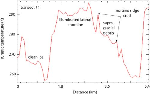
We examined kinetic temperature values from the AST08 product along two transects drawn on the temperature image in the subset area: one transverse transect across various surfaces around Zemu glacier (transect #1), and one longitudinal transect along the flowline of Zemu glacier tongue (transect #2) (Figure 6(a,b)). A first look at the ASTER temperature image (Figure 6(a)) and the two transects (Figure 6(c,d)) shows variability in the surface temperature of the supraglacial debris and surrounding areas. Figure 6(c) (transect #1) shows a large variability in temperature ranging from <260 K to >290 K, with areas <273 K (0 °C) which we associate with clean ice/snow according to the ASTER 432 color composite (Figure 6(b)). Temperature increases sharply to ∼290 K over the illuminated terrain on the northern side of Zemu glacier, followed by two distinct peaks in temperature, spaced less than 1 km apart from each other (Figure 6(c)). We associate these peaks with brightly illuminated lateral moraine ridge crests (Figure 6(b)). On Figure 6(c), we also note a directional bias in temperature, with higher temperatures on the northern moraine ridge crest than on the southern one. A look at the ASTER temperature image (Figure 6(a)) shows that the lateral slopes on the northern side of Zemu are illuminated in comparison with the southern slopes. We attribute this to topographically induced illumination effects due to the azimuth of the sun (162 degrees) at the time of the acquisition of the ASTER image (10:27 a.m. local time). Such effects are common in remote sensing images in complex mountainous terrain [15,71]. Due to such effects, the slopes facing the sun (NW in the northern hemisphere) appear to have a higher brightness than the slopes facing away from the sun (SE) during the morning hours. We estimate the area of potential debris cover on Zemu to be situated in between the two peaks in temperature noted above, roughly between 272.3 and 282.8 degrees K. This yields a width of the debris-covered tongue of ∼1 km in this cross-section of the glacier tongue.
The longitudinal kinetic temperature profile along Zemu glacier (Figure 6(d)) shows that surface temperature generally increases from ∼0 °C at the upper part of the ablation zone (in contact with the clean ice) to ∼30 °C the glacier terminus, over a distance of ∼18 km. We estimate that the upper part of Zemu glacier may be thin, and patchy, with a mixture of ice and debris pixels, which may not fully insulate the ice underneath. The low temperatures in the upper ablation area may indicate ablation rates comparable with those of clean ice, as noted in recent field-based studies on other glaciers [14,15]. On the contrary, higher temperatures at the terminus of the glacier may indicate the presence of a thick, continuous debris cover, and are in agreement with field observations from other glaciers in the Himalaya, which reported debris cover as thick as 1–2 m at the glacier termini [14,17,18]. Nakawo et al. [72] also reported a general increase in surface temperature of supraglacial debris along the glacier tongue of Khumbu glacier in Nepal, starting with ∼0°C at the contact with clean ice (Everest base camp). Recent field-based studies have confirmed this general trend of increasing ASTER temperatures with decreasing altitude, and have shown this to be related to the lower ablation rates once the debris thickness exceeds a “critical” threshold [15]. At debris thickness >0.3–0.4 m, the ice underneath is partly insulated due to the low thermal conductivity of the debris, and the surface temperature is independent of the thickness of the debris [8,9,18,73,74]. We anticipate a similar situation at the terminus of Zemu glacier, where critical thickness may be the exceeded, the cooling signal may be diminished and the ASTER temperature may no longer able to reflect the presence of the buried ice underneath.
We also note, on the two transects, that the temperature signal from the upper ablation zone to the glacier terminus is non-linear, with small rises and falls indicative of supraglacial surface features (crevassed zones, supraglacial lakes and ice walls) visible at pixel scale (Figure 6(d)) and in the field (Figure 2) [14,15]. For example, on Figure 6(d) we note a sharp depression in temperature around 6.3 km from the terminus, in the middle of the glacier, which we identified to be a supraglacial lake on the ASTER 432 color composite (Figure 6(b)). The low temperature here is possibly due to reduced latent heat due to evaporation of the lake surface, as was also observed in studies on Khumbu glacier [73] and Miage glacier [15], or to differences in emissivity of lake water versus the surrounding debris material.
The thermal analysis of debris cover has important implications: if the thermal resistivity of the debris can be measured or estimated, surface temperature data from ASTER or other sensors can be used to estimate the debris thickness and subsequently the ice ablation rates, as shown by several studies [18,73,75,76].
4.3. Decision Tree Results
The decision tree algorithm based on multi-spectral and topographic variables, and the criteria and thresholds used, are summarized in Table 2 and Figure 7. The criteria and thresholds are described in the order they were entered in the decision tree. In the final decision tree, we included eight variables, which we considered to be the most efficient at excluding areas that were not suitable for the occurrence of debris-covered ice.
- Clean ice and snow were delineated using the NDSI algorithm with a threshold of 0.7 (NDSI > 0.7 = snow/ice), as described in Section 4.1 above. Distinguishing snow from ice was not possible with NDSI alone, but both categories were excluded from potential debris at this step in the analysis.
- Clouds had a similar spectral response to ice in the visible bands (ASTER 1 and 2 in particular), but their reflectivity decreased at mid IR wavelengths. Band 4 of ASTER with a threshold of 90 successfully mapped all clouds (band 4 > 90 = clouds). However, we noted that some pixels corresponding bright moraine edges were inadequately mapped as clouds.
- Vegetation was mapped using the NDVI method with a threshold of 0.05 (NDVI < 0.05 = vegetation). The same threshold was obtained in a study conducted in the Alps [44]. Caution was exercised in choosing this threshold, because it is known that sparse vegetation can grow on some parts of the termini, covered with stagnant ice [32]. Some authors, for example, used the presence of vegetation on some parts of the debris-covered tongues during the spring time in the Kanchenjunga area as an indicator of debris to aid in the remote sensing mapping [78]. NDVI and slope variables were found to be two of the most important variables in predicting potential locations for rock glaciers in a different study [79].
- Shadows were delineated using ASTER band 3 with a threshold of 25 (band 3n < 25 = shadows). We note that shadows may occur over the debris-covered areas as well. However, the detection of debris-covered areas is not possible in areas of deep shadows anyway, unless the algorithm relies in big part on morphologic characteristics as pointed out in a few studies [32,36]. We included the shadow areas with a low threshold to exclude small, deep shadows that introduce too much noise in the final map.
- The HSV image generated from ASTER bands 2, 3 and 5 was useful for excluding bare rock and sand (including illuminated moraine) on the northern sides of the debris-covered tongues such as Zemu, using a threshold of 200 (Hue < 200 = periglacial moraine). Paul et al. [31] used the HSV image with a threshold of 126 to successfully map vegetated areas, which were then excluded from the potential debris-covered areas.
- Slope angle was calculated in GIS based on the ASTER DEM. Statistics showed that the slopes of the debris-covered areas ranged between 0 and 14 degrees. We chose a maximum value of 12 degrees in agreement with a previous studies [32], which showed that many debris cover tongues can be captured using this slope threshold. Another study, conducted in the Alps [31] used a much higher slope threshold of 24 degrees in their classification. However, we found that a higher slope threshold at this particular pixel size (30 m) included a lot of the steep slopes and rock walls with talus sheds, and were not suitable for the accumulation of debris.
- The temperature range was chosen based on bands 10 and 12 of ASTER following various experiments with all the thermal bands (section 4.2 above). Thresholding these two bands (band 10 > 70 K and band 12 < 90 K) captured most debris-covered tongues identified on the topographic map.
- Elevations outside the 4,000 m–5,600 m range were excluded from the map of potential debris-covered areas. The values are based on observations elsewhere in the Himalaya, which showed that the termini of debris-covered glaciers are generally situated between 4,000 and 5,000 m [30]. Modern ELA values were estimated to be 5,000–6,000 m in the Kangchenjunga area [79]. In a different study, we calculated a regional ELA value of ∼5,400 m for the Langtang Himalaya (in the same climatic zone as Kanchenjunga) based on ASTER imagery at the end of the ablation season [80]. The ELA was determined to be higher for debris-covered glaciers than clean glaciers for Nepal glaciers in the same climatic zone [81]. On the basis of these observations, we chose a slightly higher upper limit for the potential debris cover (5,600 m compared to 5,400 m estimated for Langtang), to minimize any exclusion of debris pixels higher in the ablation zone of glaciers.
Four of the binary outputs of the decision tree are shown as examples in Figure 8. The NDSI map (Figure 8(a)) shows snow and ice in blue, distinguished from the surrounding bare terrain, with the debris-covered tongues missing, as expected. Clouds in the southern part of the image were well delimited on the ASTER band 4 (Figure 8(b)), and vegetation in the southeastern part of the image was delineated using NDVI (Figure 8(c)). Figure 8(d) illustrates the hue component of the ASTER bands 235, which corresponds to bare rock/sand and illuminated lateral slopes.
The final debris cover map resulting from the exclusion of all eight types of unsuitable surfaces is shown in Figure 9. The upper part of the ablation zone of Zemu appears to be too cold, indicating discontinuous supraglacial debris, with exposed ice pixels. This is in agreement with previous investigations, which found thin debris in the upper part of the glacier tongues, with a temperature close to that of clean ice [18,73]. Several areas were misclassified: (a) several snow pixels in the glacier accumulation area were classified as clouds. (b) some pixels from the potentially debris-covered class were scattered throughout the image, around clouds and vegetated areas. The decision tree algorithm classified these pixels as potential debris-covered pixels. Applying a median 3 × 3 filter removed some of the noise, yielding a cleaner final map of potential debris-covered tongues (Figure 9). Parts of some debris-covered tongues were missed by the algorithm are due to either clouds (glacier #12) or shadows (glacier #11) obstructing the view of these glaciers, or the presence of thick debris. These are discussed further in Section 4.3.1 below. The decision tree algorithm resulted in 64 km2 classified as debris-covered ice, which represents 11% of the glacierized area.
4.3.1. Validation of the Decision Tree with High-Resolution Imagery
We compared the output of the decision tree with debris covered ice outlines extracted manually from the QB/WV2 imagery (Figure 10 and Table 3). The difference in the acquisition time of the ASTER and QB is < five years (November 2001–January 2006), and we don’t expect significant changes in the debris-cover extent (larger than several ASTER pixels). A visual comparison shows that in general, the debris-covered tongues were captured by the ASTER decision tree in the area of overlap of the two sets of images (Figure 10). We note that the lower parts of several debris-covered tongues were not detected (Yalung, Talung and Onglaktang), which may be due to thicker debris at the termini, partly insulating the ice underneath, as explained in Section 4.2. The middle part of Kangchenjunga glacier tongue was in shadow, and was not detected by the algorithm. Umaram Kang glacier was completely under cloud cover in the ASTER scene, and was also not detected. The upper part of the ablation area of Zemu glacier, which we identified as debris covered ice on the QB image, was classified as snow/clean ice by the ASTER algorithm, most likely due to the lower contrast of ASTER compared to the higher resolution QB image. The area of E. Rathong glacier was underestimated due to missed pixels in middle of the glacier, possibly due to thick patches of supraglacial debris in these areas.
On Table 3, we note that debris covered area estimates based on QB/WV are generally smaller than the ASTER-derived areas for all but one glacier the (E. Rathong). Overall, for the ten glacier tongues, there is an area difference of 16.2 km2 (25%) between the ASTER and the QB areas. We explain this area difference mostly as mapping errors due to clouds and shadows, or lack of contrast in the upper ablation areas, as described above. We also speculate that some glacier retreat may have occurred at the termini of these glaciers over the period November 2001–January 2006. Annual estimates of debris-covered glacier area changes in the Sikkim Himalaya are not available. Most studies report decadal area changes on the order of 18% cumulative area loss in the last three decades, or 0.6% yr−1 [13]. For Onglaktang and E. Rathong glaciers, glacier retreat on the order of 1 to 1.2 km and a cumulative area loss of ∼17 and 31% have been documented in the last two decades (1995–2005) based on field surveys [82]. This indicates annual area changes of 0.8–1.5% yr−1. Extrapolating on these studies, we assume that debris cover area changes from 2001 to 2006 may account for a maximum of ∼3–7.5% of the difference between ASTER and QB estimates, with the remaining due to the errors discussed above.
4.4. Texture Analysis Results
4.4.1. Grey-Level Co-Occurrence Measures
PCA results for the Zemu subset area are given in Figure 11. The first principal component (PC1) contains 89% of the variability present in the image (Figure 11), and hence was used for texture analysis tests using ROIs presented in section 3.3 (Figure 4). The texture images resulting from co-occurrence measures (variance, entropy and homogeneity) performed on PC1 for the subset image are shown in Figure 12(a–c). We used a window size of 3 × 3, which was large enough to capture the repeated, wave-like characteristics of the debris-covered ice, and small enough so ensure homogeneity of the surfaces within the window. The variance image (Figure 12(a)) provided the most textural information, and it showed the edges of homogenous surfaces such as lakes and clean ice. The homogeneity image (Figure 12(b)) and entropy (Figure 12(c)) image did not clearly distinguish the debris-covered tongues, and were not considered further.
A closer look at the variance image for a subset of Zemu glacier (Figure 13) reveals the presence of supra glacier lakes and ice walls characteristic of debris-covered glacier tongues. Due to the azimuth of the sun at the time of the acquisition of the ASTER image (162 degrees), the mounds on the debris surface casts a shadow visible as half-moon shapes on the zoomed images on Figure 13. Some of these mounds have steep exposed ice walls, oriented in the NE-SW direction, perpendicular to the sun azimuth, with a supraglacial lake adjacent to the ice wall. Sakai and Fujita [30] studied the orientation and melt patterns of such ice walls on Lirung and Khumbu glaciers in Nepal, and found that the majority of the ice walls were oriented northwards in the ablation season, and had steep slopes. The information about the morphologic distribution of ablation features (ice walls and supraglacial lakes) is useful for subsequently estimating surface melt of debris-covered glaciers.
Descriptive statistics of texture indices for clean ice, potentially debris-covered ice, bare rock/sand and clouds are presented in Table 4. We note some differences in the average texture indices among these regions: clean ice and clouds have low variance, low entropy and high homogeneity, which in general are characteristic of a smooth surface. Texture measures for these surfaces have long-range variability, similarly to flat terrain [48]. Debris cover, on the other hand, has the highest variance of all classes, highest entropy and lowest homogeneity compared to the other classes (mean variance of 15.27 compared to 0 for clouds and 0.06 for clean ice) (Table 4). This suggests that the debris-covered ice surfaces have a unique, irregular texture, different from clean ice and surrounding terrain.
4.4.2. Filtering in Spatial and Frequency Domain
Results of the Sobel and Roberts operators show a high density of edges per unit area for debris-covered tongues (Figure 14). The resulting grey-scale images produced by the two filters are similar to each other, with the Sobel filter producing slightly brighter edges. Clean-ice glaciers are easily distinguishable on the filtered images as black homogenous surfaces with pixel values of 0. A high concentration of edges is visible outside the clean glacier tongues, and corresponds to eroded steep slopes outside the glaciers, with lines following the direction of the rockslides. In the center of the image, the tongue of Zemu glacier is distinguishable by the bright clear moraine crest ridges. In between these ridges is very high concentration of edges with rather circular patterns, or hill-and-valley melting structures, suggestive of the presence of the debris cover. A high concentration of edges oriented east to west indicate the crevassed areas of the side tributaries of Zemu glacier. This is consistent with the complex morphology characteristic of debris cover, particularly the cones and mounds created due to accumulation of debris, and the differential melting under various debris cover thicknesses [4] (Figure 14).
Promising results of the FFT algorithm were obtained with a circular cut filter and radius of 3, which preserved the texture over the debris cover (Figure 15(a)). The results of an unsupervised classification (Isodata) on the inverse FFT image with 3 classes shows promising results for classifying debris cover and clean ice (Figure 15(b)); however, pixels from the surrounding terrain such as non-ice debris also get mixed in the classification, requiring additional processing or other criteria.
4.4.3. Geostatistics as a Texture Measure
We constructed variogram functions based on variance values from PC1 for three of the ROIs shown in Figure 4. The semivariograms with their characteristics are presented in Table 5 and Figure 16. We evaluated whether these three surfaces exhibit differences in surface characteristics, and whether these differences can be quantified with the use of the variogram. For the debris-covered area (area 1), we used a lag distance of 30 m, which corresponds to 2 ASTER pixels in the visible bands (15 m). The best fit of the data for area 1 (based on RMSE) was an exponential model with a sill of 513.6 m2, which was reached at a range of 98.7 m (∼6 pixels) (Figure 16(a)).
To check for directional dependence in the semivariogram, we computed semi-variance values for data pairs falling within certain directional bands, within the same lag distance as above (30 m). Applying a search direction of 56.3 degrees, and 3 bandwidths in fitting the model reduced the number of data pairs, and resulted in an overall better fit of the model (Figure 16(b)). The resulting variogram had a slightly lower sill (457.2 m2), a larger range (201.2 m), and a five-fold increase in the nugget compared to the one generated without a directional search. The search direction is indicative of the orientation of the surface features: in this case, this corresponds to the northeast orientation of the Zemu glacier tongue. Surface features created by ice melt (debris cones and walls) are oriented perpendicular to this direction. However, there is no clear evidence of geometrical anisotropy (Figure 16(a,b)) suggesting that the debris cover surface is rather uniform in all directions.
The high sill (457.2 m2) in conjunction with a high nugget (90.8 m) of the semivariograms for debris-covered areas determined with search direction suggests both large and small-scale (intra-pixel) variability. The large values for the sill in the semivariogram are characteristic of a rough surface, which we would expect based on the debris cover features observed in the field, such as bumps, ice wall and lakes formed by melting of the ice [83]. The high nugget value we report here can result from two phenomena [84]. The first reason for the existence of a nugget effect is random measurement errors. The second reason is that data have not been collected with a sufficiently small spacing to reveal the continuous behavior of the phenomenon, commonly referred to as subgrid variability. One way subgrid variability can be characterized is by analyzing another data set of the same phenomenon, collected at a finer sample spacing, as shown by [85], who evaluated the spatial distribution of snow depth in a seasonally snow covered catchment. We are unable to discriminate between these two possible explanations with our data sets. However, it is worth noting that the large nugget value is consistent with the rough surface that characterizes debris-covered ice. Similar patterns of complex morphology were observed in a study based on SAR data, where morphology of heavily crevassed areas or seracs could be characterized using geostatistical techniques [66]. The authors noted geometrical anisotropies on crevassed areas and seracs due to the directional dependence on the ice flow. In our case, we did not distinguish a strong geometrical anisotropy, because debris mounds and supraglacial lakes tend to be relatively symmetric and not dependent on the ice flow direction.
The variograms for the area 2 (lateral moraine, Figure 16(c)) fits an exponential model, with a progressive increase in semi-variance, and a range of 867 m, indicative of a smoother surface [85]. The semivariogram for clean ice/snow (area 3) fits a spherical model, with a large range (132 m), indicating that pixels are spatially auto-correlated over larger distances, and hence suggest a more uniform surface compared to debris-covered areas (area 1). The lower nugget values (0.7 m for clean ice and 7.8 m for lateral moraines) compared to the values debris cover (14.4/90.8 m) indicate less noise in the data in these two surfaces. The variogram of ice/snow (Figure 16d) has a very low sill compared to the other two surfaces (2.3 m). The variograms for areas 2 and 3 are isotropic, with minimal change in the sill and the shape of the variogram in different azimuthal directions. These statistics show differences in texture between debris-covered ice and clean ice or lateral moraine. However, further work is needed for an in-depth evaluation of the use of geostatistics for mapping of these features.
4.4. Comparison of Texture Analysis with the Decision Tree Results
We compared the debris cover map resulting from the variance image with the debris cover map from the decision tree. The manual delineation of debris-covered tongues from the variance image yielded 69.9 km2 of debris covered ice, which is ∼8% larger than the output of the decision tree (64.1 km2) (Table 3). A visual comparison of the decision tree output with the texture-based outlines also shows comparable results in the extent of debris cover between these two techniques (Figure 10). The glacier-by-glacier comparison of debris-covered tongues (Table 3) shows that in general, the texture analysis results yielded comparable results to the decision tree results, with differences in area between the two ranging from 0 to ∼4 km2. The main differences in area come from the upper part of the debris cover, where the rugged steep terrain or lateral moraine confounded the texture signal. Both the decision tree and the texture analysis overestimated the debris-covered area when compared to the QB/WV2 outlines by 25% and 31%, respectively (Table 3). We found that texture analysis was useful in detecting debris covered-ice in areas where the decision tree algorithm failed due to either insufficient contrast in the ASTER image (upper ablation areas) or glacier termini covered with thick debris.
5. Uncertainty and Limitations
The main sources of uncertainty in the delineation of debris cover using various techniques presented in this study come from: (1) biases in the decision tree algorithm, and the subjectivity involved in selecting the thresholds for each of the criteria used; (2) orthorectification errors inherent in the ASTER imagery and the relative DEM and (3) errors in the topographic map used to extract the a-priori knowledge. We estimate the first error to be by far the largest source of error. Unfortunately, it is difficult to assess the accuracy of the algorithm because of the lack of field-based information, partly due to the difficulty of identifying the terminus of debris-covered glaciers in the field, as noted in other studies elsewhere [86]. Errors are not spatially uniform, since they depend on the size of the glacier, the characteristics of debris cover on each glacier, and in some cases, the presence or absence of snow, shadows and clouds, which may radically increase the sources of error. Several limitations of this study are:
- Geolocation errors on the topographic map in the western part (Nepal) prevent an accurate assessment of the performance of the decision tree on these glacier tongues. Such errors are due to the use of different datums in this part of the world, most notably local datums (Everest 1956 or other), which introduce large errors when transformed to global datums (WGS84) [87].
- Profile curvature was shown to be important in previous studies to identify concavities in terrain, specific of debris-covered tongues [32,34,36,42]. Curvature was also found to be one of the most important predicting variables for debris-covered areas in other studies in the Andes [78,88]. In the current study, the profile and plan curvature calculated in GIS based on the ASTER DEM proved inconclusive in distinguishing debris-covered tongues from the surrounding terrain, as it produced noisy images. We estimate this to be caused by the noise inherent in the “relative” ASTER DEMs produced at LPDAAC, which lack post-processing steps such as terrain smoothing. Therefore, at this time, terrain curvature was not included in the decision tree.
- A quantitative assessment of the differences between the decision tree output and the old topographic map was not conducted, because of potential glacier changes that might have occurred since the 1960–1970s, and the unknown accuracy of the topographic map.
- Shadows over the debris-covered tongues remain a big problem in the delineation of these tongues. A more rigorous topographic analysis would be needed in order to capture all the debris-covered tongue independent of their degree of shadow.
- Snowfields outside the glacier caused an overestimation on the snow and ice area based on the NSDI, and had to be adjusted manually.
- Texture measures were not included in the decision tree due to the challenge of conducting texture classification and segmentation schemes. Supervised classification techniques have been used before as a visual clue to identify homogenous regions, with promising results [48]; however, these methods still require significant user input. More sophisticated methods such as structural methods, geometric methods or model-based methods also exist in other domains [46]. For debris-covered areas, we suggest that shape recognition techniques based on orientation or shading of objects may be useful to characterize the distribution of ice walls and supraglacial lakes on the texture surface. Geometrical methods such as the Voronoi polygons may also be useful for texture delimitation among regions, particularly the transition from debris cover to ice-free moraine. Voronoi polygons are areas with distinct shapes and texture derived based on texture tokens, i.e., points of high gradient or complex structure [47]. Such techniques have not yet yielded concluding results for our dataset, but will be explored in a future study.
6. Conclusions
This study compared the use of a decision tree algorithm based on multispectral and topographic data with texture analysis techniques to detect the presence of debris-covered tongues in the Kangchenjunga area of Sikkim/Nepal. The decision tree combined multi-spectral signatures, thermal characteristics and topographic criteria extracted from a DEM, and resulted in 64 km2 of debris-covered ice (11% of the glacierized area). Manual corrections were required to remove random noise, particularly in areas with deep shadow and thick debris cover. Texture analysis showed significant differences in surface characteristics of debris-covered ice (repetitive bumps, cones, wave-like structures and supraglacial lakes) compared to smoother surfaces such as snow and lateral moraines in a subset area (Zemu glaciers). Texture analysis helped detecting debris covered-ice in areas where the decision tree algorithm failed to do so, due to either the patchy supraglacial debris in the upper ablation areas of the glaciers, or the thick debris at the glacier termini. Results of the decision tree and the texture analysis for ten glaciers in the Zemu area are comparable, with only ∼8% difference in area between the two. However, when compared to high-resolution QB/WV2 images, both texture analysis and the decision tree overestimated the debris-covered area of glaciers.
Each of the two techniques presented here have some limitations, which currently make it difficult to apply these at large scales. The sophisticated and laborious processing of the decision tree prevents a completely automated process for delineating the debris-covered glacier tongues. The texture approach is limited by the fact that while debris-cover training areas (ROIs) may have distinctive texture values, these values or patterns may not be characteristic for all the debris cover across the region. Furthermore, the current challenge remains in incorporating the texture analysis results into a simple and cost-effective classification scheme. In spite of these limitations, the information generated here, particularly the thermal characteristics and the morphologic distribution of ablation features (ice walls and supraglacial lakes) helps characterizing supraglacial debris cover. Subsequently, this information can be used for estimating surface melt of debris-covered glacier tongues, which is much needed for assessing the contribution of these glaciers to water resources.
Acknowledgments
This research was funded by the NSF Doctoral Dissertation Research Improvement (DDRI) grant BCS 0728075 and a NASA Earth System Science (ESS) Fellowship 2006–2009, and a CIRES graduate fellowship from University of Colorado. Adina Racoviteanu’s current post-doctoral research is funded by the Centre National d’Études Spatiales (CNES), Paris, France. Participation of M. Williams was supported by the NSF-funded NWT LTER project and a grant from USAID. The NASA-funded Global Land Ice Monitoring from Space (GLIMS) project provided free access to ASTER data. We are grateful to Jonathan Taylor at California State University Fullerton for providing access to QuickBird and Worldview-2 imagery through the NASA Appropriations Grant NNA07CN68G, and to William Manley at Quaternary GIS Lab, University of Colorado at Boulder for his expertise and software needed to process the QB and WV2 imagery. We sincerely thank the four anonymous reviewers for their thorough comments, which helped greatly improve the quality of the manuscript, and Yves Arnaud at IRD France for his comments on an earlier version of the manuscript.
References
- Nakawo, M.; Raymond, C.F.; Fountain, A. Debris-Covered Glaciers; IAHS Press: Wallingford, UK, 2000; p. 288. [Google Scholar]
- Shroder, J.F.; Bishop, M.P.; Copland, L.; Sloan, V. Debris-covered glaciers in the Nang Parbat Himalaya, Pakistan. Geogr. Ann 2000, 82A, 17–31. [Google Scholar]
- Bishop, M.P.; Kargel, J.S.; Kieffer, H.H.; MacKinnon, D.J.; Raup, B.H.; Shroder, J.F. Remote-sensing science and technology for studying glacier processes in high Asia. Ann. Glaciol 2000, 31, 164–170. [Google Scholar]
- Iwata, S.; Aoki, T.; Kadota, T.; Seko, K.; Yamaguchi, S. Morphological Evolution of the Debris Cover on Khumbu Glacier, Nepal, between 1978 and 1995. In Debris-Covered Glaciers; Nakawo, M., Raymond, C.F., Fountain, A., Eds.; IAHS: Wallingsford, UK, 2000; Volume 264, pp. 3–11. [Google Scholar]
- Benn, D.I.; Evans, D.J.A. Glaciers and Glaciations, 2nd ed.; Hodder Arnold: London,UK, 2010. [Google Scholar]
- Casey, K.A.; Kaab, A.; Benn, D.I. Characterization of glacier debris cover via in situ and optical remote sensing methods: A case study in the Khumbu Himalaya, Nepal. The Cryosphere Dicuss 2011, 5, 499–564. [Google Scholar]
- Nakawo, M.; Yabuki, H.; Sakai, A. Characteristics of Khumbu Glacier, Nepal Himalaya: Recent change in the debris-covered area. Ann. Glaciol. 1999, 28, 118–122. [Google Scholar]
- Conway, H.; Rasmussen, L.A.; Nakawo, M. Summer Temperature Profiles within Supraglacial Debris on Khumbu Glacier, Nepal. In Debris-Covered Glaciers; Nakawo, M., Raymond, C.F., Fountain, A., Eds.; IAHS: Wallingsford, UK, 2000; pp. 89–97. [Google Scholar]
- Gades, A.; Conway, H.; Nereson, N. Radio echo-sounding through supraglacial debris on Lirung and Khumbu glaciers, Nepal Himalayas. In Debris-Covered Glaciers; Nakawo, M., Raymond, C.F., Fountain, A., Eds.; IAHS: Wallingsford, UK, 2000; pp. 13–11. [Google Scholar]
- Foster, L.A.; Brock, B.W.; Cutler, M.E.J.; Diotri, F. A physically based method for estimating supraglacial debris thickness from thermal band remote-sensing data. J. Glaciol 2012, 58, 677–690. [Google Scholar]
- Mihalcea, C.; Mayer, C.; Diolaiuti, G.; D’Agata, C.; Smiraglia, C.; Lambrecht, A.; Vuillermoz, E.; Tartari, G. Spatial distribution of debris thickness and melting from remote-sensing and meteorological data, at debris-covered Baltoro glacier, Karakoram, Pakistan. Ann. Glaciol 2008, 48, 49–57. [Google Scholar]
- Bolch, T.; Buchroithner, M.F.; Peters, J.; Baessler, M.; Bajracharya, S. Identification of glacier motion and potentially dangerous glacial lakes in the Mt. Everest region/Nepal using spaceborne imagery. Nat. Hazards Earth Syst. Sci 2008, 8, 1329–1340. [Google Scholar]
- Mool, P.K.; Bajracharya, S.R.; Joshi, S.P.; Sakya, K.; Baidya, A. Inventory of Glaciers, Glacial Lakes and Glacial Lake Outburst Floods Monitoring and Early Warning Systems in the Hindu-Kush Himalayan Region, Nepal; International Center for Integrated Mountain Development: Kathmandu, Nepal, 2002; p. 227. [Google Scholar]
- Zhang, Y.; Fujita, K.; Liu, S.; Liu, Q.; Nuimura, T. Distribution of debris thickness and its effect on ice melt at Hailuogou glacier, southeastern Tibetan Plateau, using in situ surveys and ASTER imagery. J. Glaciol 2011, 57, 1147–1157. [Google Scholar]
- Mihalcea, C.E.; Brock, B.W.; Diolaiuti, G.A.; D’Agata, C.; Citterio, M.; Kirkbride, M.P.; Cutler, M.; Smiraglia, C. Using ASTER satellite and ground-based surface temperature measurements to derive supraglacial debris covere and thickness patterns on Miage Glacier (Mont Blanc Massif, Italy). Cold Reg. Sci. Technol 2008, 52, 341–354. [Google Scholar]
- Brock, B.W.; Mihalcea, C.; Kirkbride, M.P.; Diolaiuti, G.; Cutler, M.E.J.; Smiraglia, C. Meteorology and surface energy fluxes in the 2005–2007 ablation seasons at the Miage debris-covered glacier, Mont Blanc Massif, Italian Alps. J. Geophys. Res 2010, 115, D09106. [Google Scholar]
- Takeuchi, Y.; Kayastha, R.B.; Nakawo, M. Characteristics of Ablation and Heat Balance in Debris-Free and Debris-Covered Areas on Khumbu Glacier, Nepal Himalayas, in the Pre-Monsoon Season. In Debris-Covered Glaciers; Nakawo, M., Raymond, C.F., Fountain, A., Eds.; IAHS: Wallingsford, UK, 2000; pp. 53–61. [Google Scholar]
- Kayastha, R.B.; Takeuchi, Y.; Nakawo, M.; Ageta, Y. Practical Prediction of Ice Melting Beneath Various Thickness of Debris Cover on Khumbu Glacier, Nepal, Using a Positive Degree-Day Factor. In Debris-Covered Glaciers; Nakawo, M., Raymond, C.F., Fountain, A., Eds.; IAHS: Wallingford, UK, 2000; pp. 71–81. [Google Scholar]
- Singh, P.K.; Naresh, R.K.S.; Yatveer, S. Influence of a Fine Debris Layer on the Melting of Snow and Ice on a Himalayan Glacier. In Debris-Covered Glaciers; Nakawo, M., Raymond, C.F., Fountain, A., Eds.; IAHS: Wallingford, UK, 2000; pp. 63–69. [Google Scholar]
- Bolch, T.; Kulkarni, A.; Kääb, A.; Huggel, C.; Paul, F.; Cogley, J.G.; Frey, H.; Kargel, J.S.; Fujita, K.; Scheel, M.; et al. The state and fate of Himalayan glaciers. Science 2012, 336, 310–314. [Google Scholar]
- Bolch, T.; Buchroithner, M.F.; Pieczonka, T.; Kunert, A. Planimetric and volumetric glacier changes in the khumbu himalaya since 1962 using Corona, Landsat TM and ASTER Data. J. Glaciol 2008, 54, 592–600. [Google Scholar]
- Bolch, T.; Pieczonka, T.; Benn, D.I. Multi-decadal mass loss of glaciers in the Everest area (Nepal Himalaya) derived from stereo imagery. The Cryosphere 2011, 5, 349–358. [Google Scholar] [Green Version]
- Gardelle, J.; Berthier, E.; Arnaud, Y. Slight mass gain of Karakoram glaciers in the early twenty-first century. Nature Geosci, 2012. [Google Scholar] [CrossRef]
- Berthier, E.; Arnaud, Y.; Kumar, R.; Ahmad, S.; Wagnon, P.; Chevallier, P. Remote sensing estimates of glacier mass balances in the Himachal Pradesh (Western Himalaya, India). Remote Sens. Environ 2007, 108, 327–338. [Google Scholar] [Green Version]
- Paul, F.; Haeberli, W. Spatial variability of glacier elevation changes in the Swiss Alps obtained from two digital elevation models. Geoph. Res. Lett, 2008. [Google Scholar] [CrossRef]
- Smiraglia, C.; Diolaiuti, G.; Casati, D.; Kirkbride, M.P. Recent Areal and Altimetric Variations of Miage Glacier (Monte Bianco Massif, Italian Alps). In Debris-Covered Glaciers; Nakawo, M., Raymond, C.F., Fountain, A., Eds.; IAHS: Wallingford, UK, 2000; pp. 227–233. [Google Scholar]
- Hewitt, K. The Karakoram anomaly? Glacier expansion and the ‘elevation effect’, Karakoram Himalaya. Mou. Res. Dev 2005, 25, 332–340. [Google Scholar]
- Schmidt, S.; Nusser, M. Fluctuations of Raikot Glacier during the past 70 years: A case study from the Nanga Parbat massif, northern Pakistan. J. Glaciol 2009, 55, 949–959. [Google Scholar]
- Hewitt, K. Glacier change, concentration, and elevation effects in the Karakoram Himalaya, upper Indus Basin. Mou. Res. Dev 2011, 31, 188–200. [Google Scholar]
- Sakai, A.; Fujita, K. Correspondence: Formation conditions of supraglacial lakes on debris covered glaciers in the Himalaya. J. Glaciol 2010, 56, 177–181. [Google Scholar]
- Paul, F.; Huggel, C.; Kääb, A. Combining satellite multispectral image data and a digital elevation model for mapping debris-covered glaciers. Remote Sens. Environ 2004, 89, 510–518. [Google Scholar]
- Bolch, T.; Buchroithner, M.F.; Kunert, A.; Kamp, U. Automated Delineation of Debris-Covered Glaciers Based on ASTER Data. Proceedings of 27th EARSel Symposium, Bozen, Italy, 4–7 June 2007; pp. 403–410.
- Shukla, A.; Arora, M.K.; Gupta, R.P. Synergistic approach for mapping debris-covered glaciers using optical-thermal remote sensing data with inputs from geomorphometric parameters. Remote Sens. Environ 2010, 114, 1378–1387. [Google Scholar]
- Bishop, M.P.; Bonk, R.; Kamp, U.; Shroder, J.J.F. Terrain analysis and data modeling for alpine glacier mapping. Polar. Geogr 2001, 25, 182–201. [Google Scholar]
- Paul, F.; Kaab, A.; Maisch, M.; Kellenberger, T.; Haeberli, W. Rapid disintegration of Alpine glaciers observed with satellite data. Geophy. Res. Lett, 2004. [Google Scholar] [CrossRef]
- Bolch, T.; Kamp, U. Glacier mapping in high mountains using DEMs, Landsat and ASTER data. Grazer Scriften der Geographie und Raumforschung 2006, Band 41. 37–48. [Google Scholar]
- Bishop, M.P.; Bonk, R.; Kamp, U., Jr.; Shroder, J.F., Jr. Terrain analysis and data modeling for alpine glacier mapping. Polar Geogr 2001, 25, 182–201. [Google Scholar]
- Racoviteanu, A.; Paul, F.; Raup, B.; Khalsa, S.J.S.; Armstrong, R. Challenges and recommendations in mapping of glacier prameters from space: Results of the 2008 global land ice measurements frpom space (GLIMS) workshop, Boulder, Colorado, USA. Ann. Glaciol 2009, 50, 53–69. [Google Scholar]
- Paul, F.; Barrand, N.; Berthier, E.; Bolch, T.; Casey, K.; Frey, H.; Joshi, S.P.; Konovalov, V.; Bris, R.L.; Mölg, N.; et al. On the accuracy of glacier outlines derived from remote sensing data. Ann. Glaciol 2012, 54. in press.. [Google Scholar]
- Suzuki, R.; Fujita, K.; Ageta, Y. Spatial distribution of thermal properties on debris-covered glaciers in the Himalayas derived from ASTER data. Bull. Glacier. Res 2007, 24, 13–22. [Google Scholar]
- Racoviteanu, A.; Williams, M.W.; Barry, R. Optical remote sensing of glacier mass balance: A review with focus on the Himalaya. Sensors 2008, 8, 3355–3383. [Google Scholar]
- Kamp, U.; Byrne, M.; Bolch, T. Glacier fluctuations between 1975 and 2008 in the Greater Himalaya Range of Zanskar, southern Ladakh. J. Mou. Sci 2011, 8, 374–389. [Google Scholar]
- Shukla, A.; Gupta, R.P.; Arora, M.K. Estimation of debris cover and its temporal variation using optical satellite sensor data: A case study in Chenab basin, Himalaya. J. Glaciol 2009, 55, 444–452. [Google Scholar]
- Taschner, S.; Ranzi, R. Landsat-TM and ASTER Data for Monitoring a Debris Covered Glacier in the Italian Alps within the GLIMS Project. Proceedings of 2002 IEEE International Geoscience and Remote Sensing Symposium, Toronto, ON, Canada, 24– 28 June 2002; 4, pp. 1044–1046.
- Brenning, A.; Peña, M.A.; Long, S.; Soliman, A. Thermal remote sensing of ice-debris landforms using ASTER: An example from the Chilean Andes. The Cryosphere, 2012. [Google Scholar] [CrossRef]
- Nakawo, M.; Morohoshi, T.; Uehara, S. Satellite Data Utilization for Estimating Ablation of Debris Covered Glaciers. Proceedings of the Kathmandu Symposium, Kathmandu, Nepal, 16–21 November 1992; 218, pp. 75–83.
- Tuceryan, M.; Jain, A.K. Texture Analysis. In The Handbook of Pattern Recognision and Computer Vision, 2nd ed.; Chen, C.H., Pau, L.F., Wang, P.S.P., Eds.; World Scientific Publishing: Singapore, 1998; pp. 207–248. [Google Scholar]
- Chica-Olmo, M.; Abarca-Hernandez, F. Variogram Derived Image Texture for Classifying Remotely Sensed Images. In Remote Sensing Image Analysis: Including the Spatial Domain; de Jong, S.M., van der Meer, F.D., Eds.; Kluwer Academic Publishers: Dordrecht, The Netherlands, 2004; pp. 93–111. [Google Scholar]
- Rignot, E.; Kwok, R. Extraction of Textural Features in SAR Images: Statyistical Model and Sensitivity. Proceedings of 10th Annual International Geoscience and Remote Sensing Symposium, Washington, DC, USA, 20– 24 May 1990; pp. 1979–1982.
- Soares, J.V.; Rennó, C.D.; Formaggio, A.R.; Yanasse, C.D.F.; Frery, A.C. An investigation of the selection of texture features for crop discrimination using SAR imagery. Remote Sens. Environ 1997, 59, 234–247. [Google Scholar]
- Chamundeeswari, V.V.; Singh, D.; Singh, K. An analysis of texture measures in PCA-based unsupervised classification of SAR images. IEEE Trans. Geosci. Remote Sens 2009, 6, 214–218. [Google Scholar]
- Frey, H.; Paul, F.; Strozzi, T. Compilation of a glacier inventory for the western Himalayas from satellite data: Methods, challenges and results. Remote Sens. Environ 2012, 124, 832–843. [Google Scholar]
- Racoviteanu, A.; Williams, M.W.; Barry, R. Optical remote sensing of glacier mass balance: A review with focus on the Himalaya. Sensors 2008, 8, 3355–3383. [Google Scholar]
- Ageta, Y.; Higuchi, K. Estimation of mass balance components of a summer-accumulation type glacier in the nepal himalaya. Geogr. Ann. Ser. A-Phyl. Geogr 1984, 66, 249–255. [Google Scholar]
- Kaul, M.K.; Puri, V.M.K. Inventory of Himalayan Glaciers: A Contribution to the International Hydrological Programme; Sangewar, C.V., Shukla, S.P., Eds.; Geological Survey of India: Kolkata, India, 1999. [Google Scholar]
- Srikantia, S.V. Restriction on maps: A denial of valid geographic information. Curr. Sci 2000, 79, 484–488. [Google Scholar]
- Survey of India. National Map Policy. 2005. Available online: http://www.surveyofindia.gov.in/tenders/nationalmappolicy/nationalmappolicy.pdf (accessed on 24 October 2010).
- Jarvis, A.; Reuter, H.I.; Nelson, A.; Guevara, E. Hole-Filled SRTM for the Globe Version 4 Available from the CGIAR-CSI SRTM 90 m Database. Available online: http://srtm.csi.cgiar.org (accessed on 2 June 2012).
- Manley, W.F. Geospatial Inventory Analysis of Glaciers: A Case Study for the Eastern Alaska Range. In Satellite Image Atlas of Glaciers of the World: US Geological Survey Professional Paper 1386-K; Williams, R.S., Jr., Ferrigno, J.G., Eds.; USGS: Denver, CO, USA, 1988; pp. K424–K439. [Google Scholar]
- LPDAAC. ASTER Digital Elevation Model–AST14DEM-Relative. Available online: http://asterweb.jpl.nasa.gov/content/03_data/01_Data_Products/release_DEM_relative.htm. (accessed on 27 September 2012).
- Digital Globe. QuickBird Imagery Products–Product Guide. Revision 4.7.3. 2007. Available online: http://www.hatfieldgroup.com/UserFiles/File/GISRemoteSensing/ResellerInfo/QuickBird/QuickBird%20Imagery%20Products%20-%20Product%20Guide.pdf (accessed on 2 June 2012).
- Hall, D.K.; Chang, A.T.C.; Siddalingaiah, H. Reflectances of glaciers as calculated using Landsat-5 thematic mapper data. Remote Sens. Environ 1988, 25, 311–321. [Google Scholar]
- Hall, D.K.; Riggs, A.G.; Salomonson, V.V. Development of methods for mapping global snow cover using moderate resolution imaging spectroradiometer data. Remote Sens. Environ 1995, 54, 127–140. [Google Scholar]
- Paul, F.; Kääb, A.; Maisch, M.; Kellenberger, T.; Haeberli, W. The new remote-sensing-derived Swiss glacier inventory: I. Methods. Ann. Glaciol 2002, 34, 355–361. [Google Scholar] [Green Version]
- Lillesand, T.; Kiefer, R.W.; Chipman, J. Remote Sensing and Image Interpretation, 6th ed.; John Wiley & Sons: New York, NY, USA, 2008. [Google Scholar]
- Hertzfeld, U.C.; Stauber, M.; Stahl, N. Geostatistical characterization of ice surfaces from ERS-1 and ERS-2 SAR data, Jakobsavn Isbrae, Greenland. Ann. Glaciol 2000, 30, 224–233. [Google Scholar]
- Atkinson, P.M.; Tate, N.J. Spatial scale problems and geostatistical solutions: A review. Prof. Geogr 2000, 54, 607–623. [Google Scholar]
- Racoviteanu, A.; Arnaud, Y.; Williams, M. Decadal changes in glacier parameters in Cordillera Blanca, Peru derived from remote sensing. J. Glaciol 2008, 54, 499–510. [Google Scholar]
- Dozier, J. Spectral signature of alpine snow cover from the Landsat thematic mapper. Remote Sens. Environ. 1989, 28, 9–22. [Google Scholar]
- Kääb, A. Combination of SRTM3 and repeat ASTER data for deriving alpine glacier flow velocities in the Bhutan Himalaya. Remote Sens. Environ 2005, 94, 463–474. [Google Scholar]
- Richter, R. Correction of atmospheric and topographic effects for high spatial resolution satellite imagery. Int. J. Remote Sens 1997, 18, 1099–1111. [Google Scholar]
- Nakawo, M.; Yabuki, H.; Sakai, A. Characteristics of Khumbu Glacier, Nepal Himalaya: Recent change in the debris-covered area. Ann. Glaciol 1999, 28, 118–122. [Google Scholar]
- Nakawo, M.; Rana, B. Estimate of ablation rate of glacier ice under a supraglacial debris layer. Geogr. Ann. Ser. A-Phy. Geogr 1999, 81, 695–701. [Google Scholar]
- Mattson, L.E.; Gardner, J.S.; Young, G.J. Ablation on Debris Covered Glaciers: An Example from the Rakhiot Glacier, Panjab, Himalaya. Proceedings of the International Symposium, Kathmandu, Nepal, 16–21 November 1992.
- Lambrecht, A.; Mayer, C.; Hagg, W.; Popovnin, V.; Rezepkin, A.; Lomidze, N.; Svanadze, D. A comparison of glacier melt on debris-covered glaciers in the northern and southern Caucasus. The Cryosphere 2011, 5, 525–538. [Google Scholar] [Green Version]
- Nakawo, M.; Morohoshi, T.; Uehara, S. Satellite Data Utilization for Estimating Ablation of Debris Covered Glaciers. Proceedings of the International Symposium on Snow and Glacier Hydrology, Kathmandu, Nepal, 16–21 November 1992; pp. 75–83.
- Kulkarni, A.V.; Bahuguna, I.M. Glacial retreat in the Baspa basin, Himalaya, monitored with satellite stereo data. J. Glaciol 2002, 48, 171–172. [Google Scholar]
- Brenning, A. Benchmarking classifiers to optimally integrate terrain analysis and multispectral remote sensing in automatic rock glacier detection. Remote Sens. Environ 2009, 113, 239–247. [Google Scholar]
- Benn, D.; Owen, L.A. Equilibrium-line altitudes of the Last Glacial Maximum for the Himalaya and Tibet: an assessment and evaluation of results. Quatern. Int 2005, 138–139, 55–58. [Google Scholar]
- Racoviteanu, A.; Armstrong, R.; Williams, M. Assessing the contribution of ice-melt to streamflow in the Himalaya using remote sensing and isotopic analysis. Water Resour. Res, 2012; submitted. [Google Scholar]
- Kayastha, R.B.; Harrison, S.P. Changes of the equilibrium-line altitude since the Little Ice Age in the Nepalese Himalaya. Ann. Glaciol 2008, 48, 93–99. [Google Scholar]
- Chattopadhyay, G.P. Recent retreats of glaciers on the southeast-facing slopes of the Kanchenjunga Summit Complex in the Sikkim Himalaya. Himalayan Geol 2008, 29, 171–176. [Google Scholar]
- Sakai, A. Distribution characteristics and energy balance of ice cliffs on debris-covered Glaciers, Nepal Himalaya. Arctic Antart. Alp. Res 2002, 34, 12–19. [Google Scholar]
- Western, A.W.; Bloschl, G.; Grayson, R.B. Geostatistical characterisation of soil moisture patterns in the Tarrawarra a catchment. J. Hydrol 1998, 205, 20–37. [Google Scholar]
- Erikson, T.A.; Williams, M.; Winstral, A. Persistence of topographic controls on the spatial distribution of snow in rugged mountain terrain, Colorado, United States. Water Resour. Res 2005. [Google Scholar] [CrossRef]
- Paul, F. New Swiss Glacier Inventory 2000-Application of Remote Sensing and GIS. In Schriftenreihe Physische Geographie; Universität Zürich: Zürich, Switzerland, 2003; p. 210. [Google Scholar]
- Srivastava, B.K.; Ramalin, K. Error Estimates for WGS-84 and Everest (India-1956) Transformation. Available online: http://www.geospatialworld.net/index.php?option=com_content&view=article&id=14377%3Aerror-estimates-for-wgs-84-and-everest-india-1956-transformation&catid=89%3Atechnology-image-processing&Itemid=50 (accessed on 2 June 2012).
- Brenning, A.; Trombotto, D. Logistic regression modeling of rock glacier and glacier distribution: Topographic and climatic controls in the semi-arid Andes. Geomorphology 2006, 81, 141–154. [Google Scholar]
Figure 1.
Location map of the study area (the Sikkim Himalaya). The figure on the right is a false color composite (FCC) ASTER 543. In this composite, glacier ice is shown as turquoise, vegetation is green, clouds are white and bare land is red. The yellow arrow points to the clouds obstructing the view of glaciers on the southern part of the image. Also shown is the subset area on which texture analysis was performed (Section 2.4). Numbers refer to glaciers mentioned in the text: 1- S.Lonak; 2- Broken; 3- E.Langpo; 4-Ramtang; 5-Yalung; 6-Zemu; 7-Tongshuong; 8-Talung; 9-E.Rathong; 10-Onglaktang; 11-Kangchenjunga; 12-Umaram Kang.
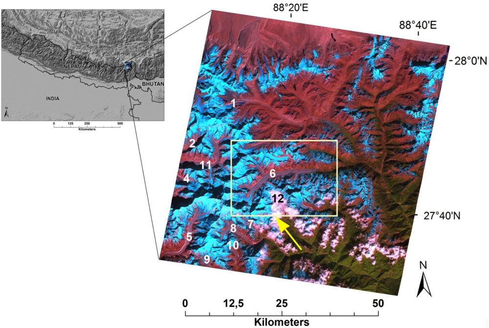
Figure 2.
A section of the debris covered tongue of Onglaktang glacier, seen from Goecha La (∼5,300 m). The morphology of the debris-cover tongue is visible as cones and mounds (A), and ice walls (B). Also visible is the sharp moraine ridge crest (C), lateral (periglacial) moraine (D) and seasonal snow on the glacier tongue and on the lateral moraines (E). The photograph was taken in November 2006.

Figure 3.
Sikkim section of the Swiss Foundation for Alpine Research topographic map at 1:150,000 used as baseline data in this study. Black solid lines represent glaciers digitized manually from the 1970s topographic map.
Figure 3.
Sikkim section of the Swiss Foundation for Alpine Research topographic map at 1:150,000 used as baseline data in this study. Black solid lines represent glaciers digitized manually from the 1970s topographic map.
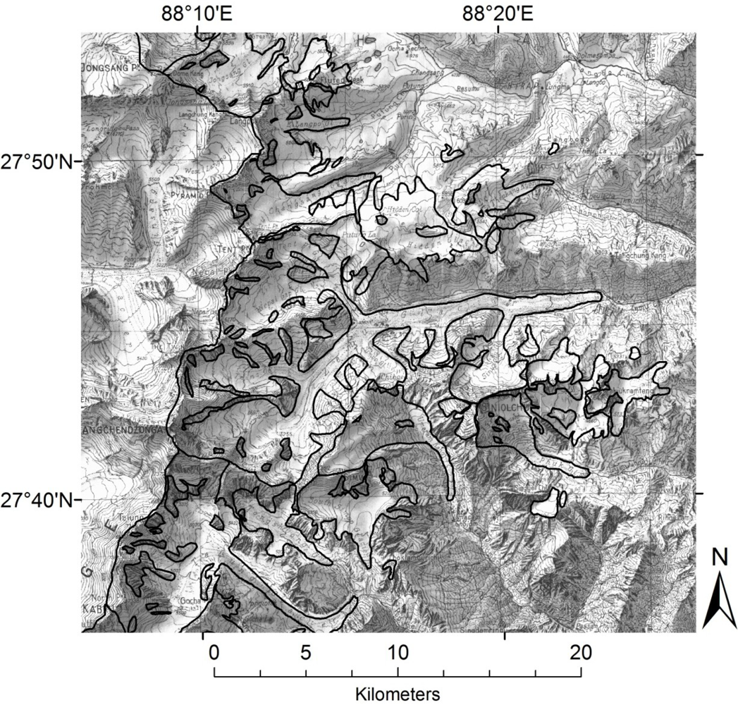
Figure 4.
ASTER color composite 321 showing ROIs digitized manually and shown as solid polygons: Debris (red), snow/ice (blue), bare rock and sand (yellow) and clouds (magenta) were digitized and all four classes were used for the GCLM texture measures; only the first three classes were used for the geostatistical analysis (Section 4.4.3).

Figure 5.
Results of the clean ice/snow delineation based on the 2001 ASTER scene, using the NDSI algorithm. The letters point to: A-correctly classified clean ice and snow; B-proglacial lakes misclassified as snow/ice; C-shadows on glacier surface; D-nunataks; E-debris covered tongue of Zemu glacier, missed by the NDSI algorithm; F-transient snow misclassified as glacier ice and G- clouds. Adapted from Racoviteanu et al. [41].
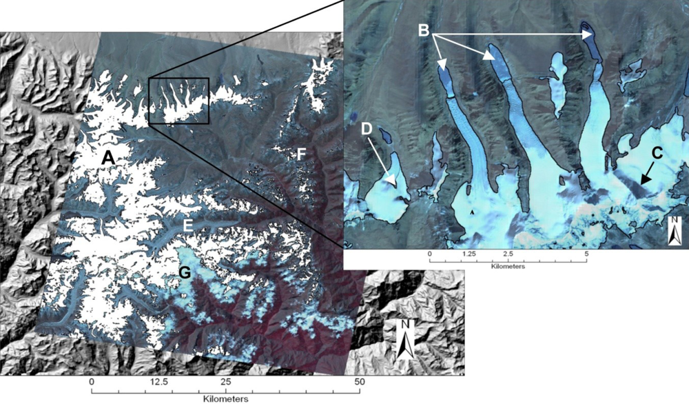
Figure 6.
(a) AST08 product (kinetic temperature band) for Zemu glacier, with two transects: across the Zemu glacier and surroundings (transect #1, in red) and along the glacier (transect #2, in green); (b) ASTER color composite 432 shown for comparison; (c) surface temperature across Zemu and surrounding surfaces (direction NW to SE); on the lower left graph, we point to the sharp lateral moraine ridge crests visible on as bright pixels on the surface temperature image; (d) surface temperature along the tongue of Zemu glacier (direction SW to NE). Surface temperature generally increases towards the glacier terminus, indicating a thicker debris cover.
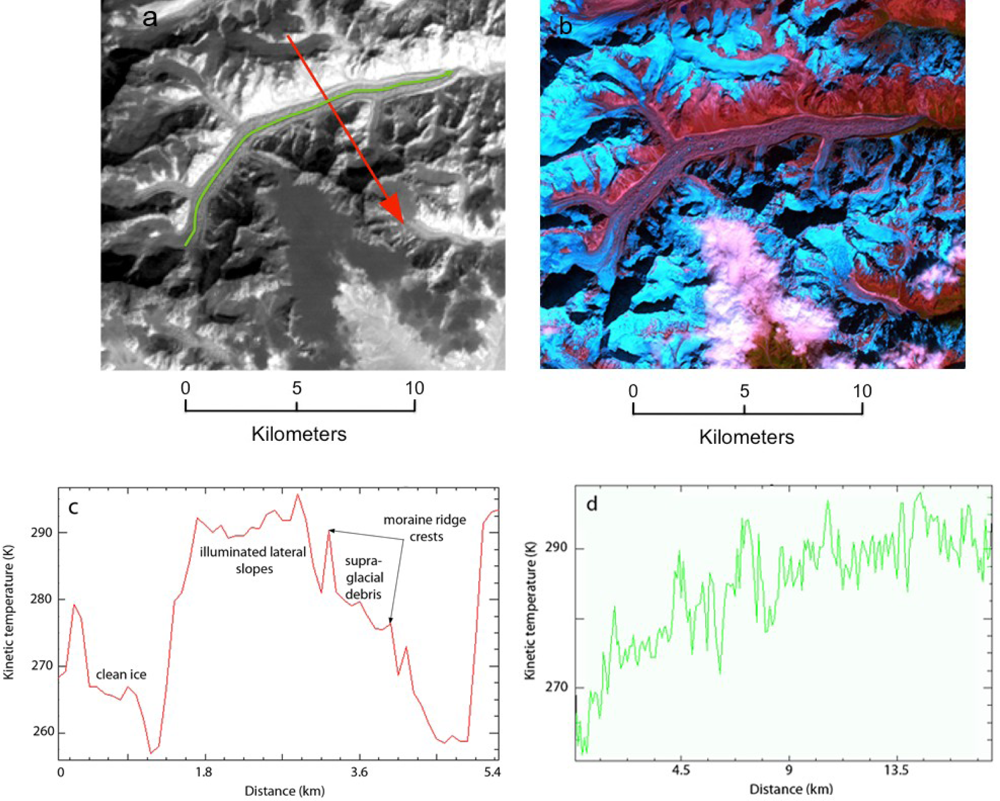
Figure 7.
The ENVI decision tree based on topographic and multispectral criteria and thresholds. Each criteria consist in a conditional statement (left side ellipsoids). Every time a condition is fulfilled, the resulting class/binary map (right side rectangular boxes) is excluded from the area of potential debris, resulting in a final map of suitable areas for debris cover.

Figure 8.
Four of the classes resulting from the multispectral criteria, shown as examples of the output of the criteria in the decision tree in Figure 7: (a) NDSI map with clean glacier areas in blue; (b) ASTER band 4 with cloud outlines in yellow; (c) NDVI map with vegetation mask in green and (d) HSV 235 color transform with the hue component for non-vegetated bare rock/sand shown in red.

Figure 9.
Results of the decision tree classification for the 2001 ASTER scene. Potential debris covered ice is shown in red, and is overlayed on a 321 color composite of the ASTER scene.
Figure 9.
Results of the decision tree classification for the 2001 ASTER scene. Potential debris covered ice is shown in red, and is overlayed on a 321 color composite of the ASTER scene.

Figure 10.
Comparison of debris covered glacier outlines derived from the decision tree with manually derived QB-WV2 outlines, shown on a color composite (QB bands 432). The transparent box marks the area outside the ASTER image, with glaciers that were not included in this comparison. Numbers refer to glaciers mentioned in the text and on Figure 1: 1- S.Lonak; 2- Broken; 3- E.Langpo; 4-Ramtang; 5-Yalung; 6-Zemu; 7-Tongshuong; 8-Talung; 9-E.Rathong; 10-Onglaktang; 11-Kangchenjunga; 12-Umaram Kang.
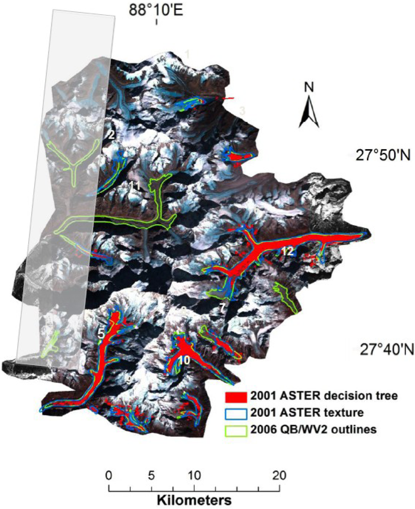
Figure 11.
Scree plot of eigenvalues resulting from the PCA analysis of the visible and shortwave infrared ASTER bands (x-axis) and the variability explained by each component (y-axis).
Figure 11.
Scree plot of eigenvalues resulting from the PCA analysis of the visible and shortwave infrared ASTER bands (x-axis) and the variability explained by each component (y-axis).

Figure 12.
Three co-occurrence grey level measures derived from PC1 of the subset image (all with a 3 × 3 moving window: (a) variance; (b) homogeneity; (c) entropy.
Figure 12.
Three co-occurrence grey level measures derived from PC1 of the subset image (all with a 3 × 3 moving window: (a) variance; (b) homogeneity; (c) entropy.
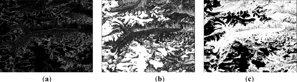
Figure 13.
(left) Variance measure derived from PC1 using a 3 × 3 moving window zoom, shown for the middle section of. The distinct pattern of supraglacial lakes is visible as circular features. Labels on the zoomed figures point to: 1-a supraglacial lake on the north side of the ice wall; 2-moon-shaped ice walls shown on the variance image (upper right) and original ASTER 321 color composite (lower right). The arrow points in the direction of the sunlight at the time of acquisition of the image (sun azimuth = 162 degrees).

Figure 14.
Results of the Sobel filter using a 3 × 3 moving window over the subset image. Debris cover is distinguished by a higher concentration of edges, including circular features (supraglacial lakes). Crevasses are also visible in this image, as a concentration of edges transversal to the flow direction.
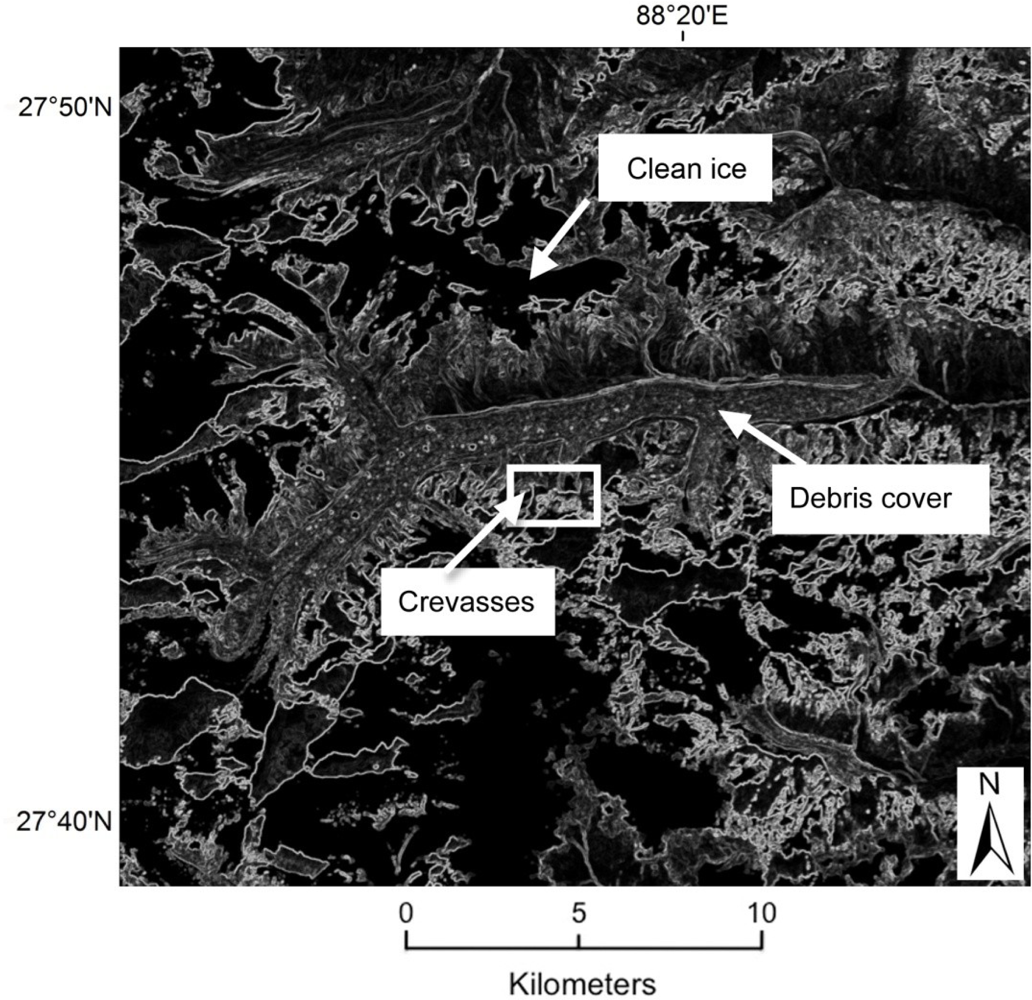
Figure 15.
(a) Inverse FFT image obtained from band 1 of ASTER, using a circular cut filter; (b) unsupervised classification applied to the inverse FFT image. Clean ice and debris-covered areas are depicted in red; surrounding periglacial moraines in magenta; ice in shadow and supraglacial lakes in green; (c) color composite of QB 432 and black and white WV2 imagery for the Zemu glacier, shown here for visual comparison.
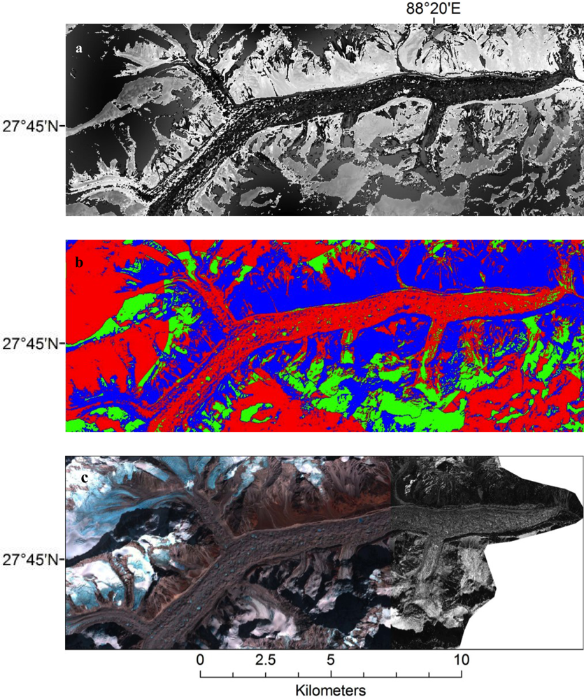
Figure 16.
Semivariograms constructed from PC1 for three of the surface types in Figure 4: (a) semivariogram for debris-covered ice with no search direction; (b) semivariogram for debris-covered ice with search direction; (c) bare rock/sand outside the glaciers and (d) ice/snow in the accumulation area of glaciers.


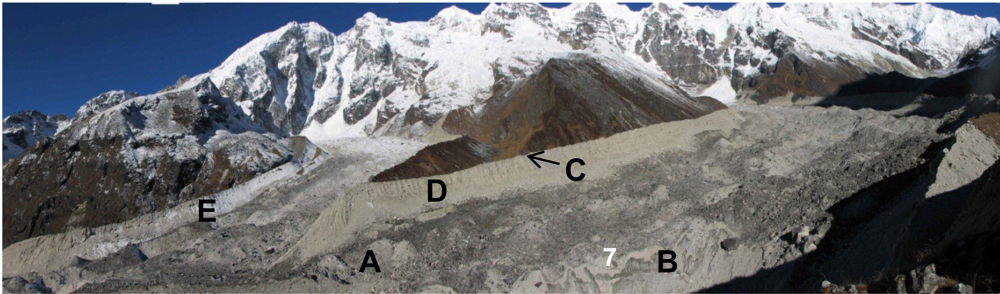
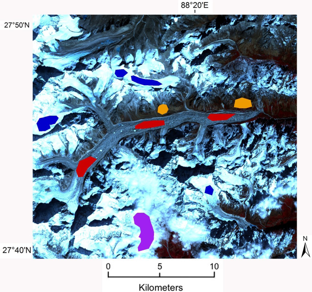
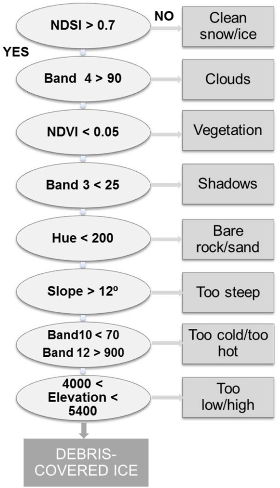
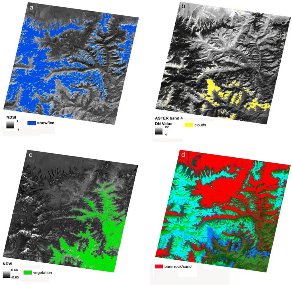
| Source | Scene ID | Date | Spatial Resolution | Notes |
|---|---|---|---|---|
| ASTER | AST14DMO_00311272001045729_20071114145408 | 11-26-2001 | 15 m VIS 30 m SWIR 90 TIR | Some seasonal snow; clouds on the lower part of the image mostly outside glaciers |
| Quickbird | 1010010004BD8700 1010010004BB8F00 | 1-6-2006 1-1-2006 | 2.4 m multispectral | Well contrasted; no clouds; minimal snow |
| WorldView2 | 102001000FBA1D00 | 12-02-2010 | 0.5 m panchromatic | No clouds; good contrast |
| Topographic map | N/A | ∼1960s–1970s | - | Exact date of the source aerial photography unknown; used as a priori knowledge to extract various classes. |
| Criteria | ASTER Bands | Range | Threshold | Justification |
|---|---|---|---|---|
| Snow/ice | NDSI (bands 1 and 4) | 0.72–1 | 0.7 | Reflective in the VIS and less reflective in the NIR |
| Clouds | Band 4 | 76–141 | 90 | Reflective in mid-IR where the reflectivity of snow and ice decreases |
| Vegetation | NDVI (bands 2 and 3) | 0.05–0.56 | 0.05 | Highly reflective in the NIR, less in the VIS |
| Shadows | Band 3 | 2–30 | 25 | Shadows are most distinguishable in band 3, where they have low reflectance values |
| Hue | HSV (bands 235) | 210–258 | 200 | Useful for distinguishing between vegetated and non-vegetated land |
| Slope | ASTER DEM | 0–14 | 12 | Debris-cover tongues generally have gentle slopes |
| Temperature | AST08; bands 10–12 | 272.3–282.8 K | Band 10 > 700 and band 12 < 900 | Debris covered ice generally colder than lateral moraines for thin patchy debris |
| Elevation | ASTER DEM | 4,000–5,400 | 4,000–5,400 | Debris-covered tongues exist between regional minimum termini elevation and below the regional ELA |
Table 3.
Comparison between the debris-covered areas based on ASTER decision tree with manually digitized areas from QB/WV2 and the ASTER texture analysis for the ten selected glaciers. Kangchenjunga glacier (#11) and Umaram Kang glacier (#12) were not included here because they were in shadow and under cloud cover, respectively.
| ID | Glacier | 2001 ASTER (Decision Tree) (km2) | 2001 ASTER Texture (Manual) (km2) | Area Difference (Texture-Decision Tree) (km2) | 2006 QB/WV2 (Manual) (km2) |
|---|---|---|---|---|---|
| 1 | S. Lhonak | 0.9 | 1.2 | 0.3 | 0.8 |
| 2 | Broken | 2.6 | 3.0 | 0.4 | 0.2 |
| 3 | E. Langpo | 2.2 | 2.4 | 0.2 | 1.7 |
| 4 | Ramtang | 1.1 | 2.4 | 1.3 | 0.7 |
| 5 | Yalung | 13.2 | 16.9 | 3.7 | 9.0 |
| 6 | Zemu | 24.7 | 24.8 | 0.1 | 20.1 |
| 7 | Tongshuong | 4.0 | 2.2 | −1.8 | 2.2 |
| 8 | Talung | 9.9 | 10.1 | 0.2 | 7.7 |
| 9 | E. Rathong | 2.7 | 3.9 | 1.2 | 3.5 |
| 10 | Onglaktang | 2.9 | 2.9 | 0.0 | 2.0 |
| Total | 64.1 | 69.9 | 5.7 | 47.9 | |
Table 4.
Mean statistics for three texture indices (co-occurrence values) for the Zemu subset image. Statistics are derived from the regions of interest (ROIs) shown in Figure 4.
| Clean Ice | Debris Cover | Clouds | Bare Rock/Sand | |
|---|---|---|---|---|
| Variance | 0.06 | 15.27 | 0 | 2.01 |
| Homogeneity | 0.99 | 0.22 | 1 | 0.52 |
| Entropy | 0.01 | 2.13 | 0 | 1.79 |
Table 5.
Variogram characteristics of the three types of surfaces extracted from PC1 and three regions of interest (ROIs).
| Search Direction | Shape | Nugget (m) | Sill (m2) | Range (m) | |
|---|---|---|---|---|---|
| Debris | no | Exponential | 14.4 | 513.6 | 98.7 |
| Debris | yes | Exponential | 90.8 | 457.2 | 201.2 |
| Bare Rock/Sand | no | Exponential | 7.8 | 48.2 | 87 |
| Clean ice | no | Spherical | 0.7 | 2.3 | 132 |
Share and Cite
MDPI and ACS Style
Racoviteanu, A.; Williams, M.W. Decision Tree and Texture Analysis for Mapping Debris-Covered Glaciers in the Kangchenjunga Area, Eastern Himalaya. Remote Sens. 2012, 4, 3078-3109. https://doi.org/10.3390/rs4103078
AMA Style
Racoviteanu A, Williams MW. Decision Tree and Texture Analysis for Mapping Debris-Covered Glaciers in the Kangchenjunga Area, Eastern Himalaya. Remote Sensing. 2012; 4(10):3078-3109. https://doi.org/10.3390/rs4103078
Chicago/Turabian StyleRacoviteanu, Adina, and Mark W. Williams. 2012. "Decision Tree and Texture Analysis for Mapping Debris-Covered Glaciers in the Kangchenjunga Area, Eastern Himalaya" Remote Sensing 4, no. 10: 3078-3109. https://doi.org/10.3390/rs4103078