Understanding and Ameliorating Non-Linear Phase and Amplitude Responses in AMCW Lidar

School of Engineering, The University of Waikato, Private Bag 3105, Hamilton 3240, New Zealand
*
Author to whom correspondence should be addressed.
Remote Sens. 2012, 4(1), 21-42; https://doi.org/10.3390/rs4010021
Submission received: 16 November 2011
/
Revised: 9 December 2011
/
Accepted: 16 December 2011
/
Published: 23 December 2011
(This article belongs to the Special Issue Time-of-Flight Range-Imaging Cameras)
Abstract
:Amplitude modulated continuous wave (AMCW) lidar systems commonly suffer from non-linear phase and amplitude responses due to a number of known factors such as aliasing and multipath inteference. In order to produce useful range and intensity information it is necessary to remove these perturbations from the measurements. We review the known causes of non-linearity, namely aliasing, temporal variation in correlation waveform shape and mixed pixels/multipath inteference. We also introduce other sources of non-linearity, including crosstalk, modulation waveform envelope decay and non-circularly symmetric noise statistics, that have been ignored in the literature. An experimental study is conducted to evaluate techniques for mitigation of non-linearity, and it is found that harmonic cancellation provides a significant improvement in phase and amplitude linearity.
1. Introduction
Time-of-Flight (ToF) full-field range imaging cameras measure the distance to objects in the scene for every pixel in an image simultaneously. This is achieved by illuminating the scene with intensity modulated or encoded light, and imaging the backscattered light using a specialised gain modulated image sensor, allowing measurement of the illumination time-of-flight, and thus distance. This technology has matured to a level where it is generating interest in consumer and industrial applications. A number of manufacturers are offering off-the-shelf range-imaging cameras or development systems intended as demonstrators or reference designs for product designers. Although most commercial ToF cameras can achieve subcentimetre measurement precision, accuracy is often an order of magnitude worse due to non-linear range responses. These errors are a significant factor in limiting uptake of full-field range imaging technology in many application areas.
Linearity can be affected by mechanisms either external or internal to the camera. The most significant external influence is generally multi-path or mixed pixel interference, where the distance measurement is perturbed by stray light or multiple returns at object edges; these are extremely scene dependent and unpredictable. This paper focuses primarily on linearity errors due to internal influences, and hence these external mechanisms will not be considered in any depth.
In the idealised case, a scene is illuminated with sinuisoidally modulated light; ranging is achieved by deducing the time delay introduced by the distance travelled. Because it is very difficult to directly measure the phase and amplitude of a high frequency signal across a 2D field-of-view, Amplitude Modulated Continuous Wave lidar detectors operate by indirectly measuring the backscattered illumination. Range measurements are performed by correlating the detected illumination signal at the sensor with a reference signal, and integrating over time. By changing the phase of the reference signal, it is possible to determine the time-of-flight. Commercial range cameras typically achieve this by acquiring four images at 90 degree phase offsets. The negative fundamental bin of a Fourier transform is calculated for every pixel revealing the amplitude and phase information, effectively performing double quadrature detection on the detected illumination.
Internal sources of linearity errors are predominantly influenced by the illumination and sensor modulation waveform shapes; in particular, the level of harmonic content. In an ideal case, pure sinusoidal modulation would result in excellent measurement linearity, but in real-world devices sinusoidal modulation is difficult to achieve due to nonlinear pixel and illumination modulation responses. Square wave modulation is much more practical because square signals can be generated easily with digital electronics. However, because only four samples are acquired per cycle, any odd harmonics present in the correlated waveforms are aliased onto the fundamental, interfering with the measurements and causing linearity errors. These linearity errors are generally viewed as well behaved and predictable; hence manufacturers typically mitigate these effects with fixed calibration tables. However, because the modulation waveforms can change due to factors such as operating frequency and temperature, typical calibrations are only valid for specific, limited operating conditions. In order to ensure robust calibration, given process variation, each camera needs to be individually calibrated, which can impact on the efficiency of the manufacturing process. With demand for ever-increasing accuracy, high quality modelling and mitigation of linearity errors is increasing in importance.
Ideally, linearity errors should be addressed at their source, rather than compensated for by calibration. Several techniques have recently been published for addressing the sources of calibration: including heterodyning and harmonic cancellation. In this paper we first discuss the sources of linearity errors and the principles behind removing them. In particular, we introduce explanations for integration time dependent aliasing and cyclic errors which cannot be explained merely by aliasing.
This paper discusses the causes of non-linear phase and amplitude responses, which can be categorised by plotting the phase and amplitude error over a full phase cycle, ideally using a translation stage. From a diagnostic perspective, many different properties of the system can be inferred from a phase sweep. Linear errors over a phase sweep are generally due to temperature drift over the experiment or due to mixed pixel/multipath interference. In either case, the two ends of the sweep do not join together. Errors composed of a single cycle in amplitude and phase over the entire 2π sweep are generally due to mixed pixels/multipath interference. For four phase steps systems: four, eight or 4n cycle errors are mostly due to aliasing of correlation waveform harmonics. Any other frequencies, in particular two cycle errors, are caused by irregular phase steps due to crosstalk or changes in the illumination modulation envelope and waveform shape between phase steps.
In Section 2 we start by developing a detailed model for measurement formation, detailing both the idealised case and the practical impacts of real sampling methodologies. Section 3 gives a comprehensive overview of known and new linearity error sources in AMCW lidar systems, starting by covering the well-known problem of the aliasing of correlation waveform harmonics. Standard methods of correction for this problem are detailed, as well as their limitations; these limitations include spatiotemporal variation in correlation waveform shape, which is frequently ignored as a factor by calibration based correction methods. New linearity error sources are discussed; in particular, crosstalk and modulation envelope decay and non-circularly-symmetric noise statistics, generally caused by the presence of a second harmonic in the correlation waveform. Finally, Section 4 details advanced methods of aliasing mitigation.
2. Background Theory
Functions of a discrete variable are notated as f[x], whereas functions of a continuous variable are notated as f(x). The Fourier transform of a function f(x) is written F (u). We take j2 = −1 and f* to be the complex conjugate of f.
2.1. Formation of the Correlation Waveform
The scene is illuminated with a modulated waveform which is reflected by the scene back to the sensor. The time-of-flight to the scene and back to the sensor is encoded as a phase shift of the received modulated signal.
Let ψi(ϕ) be the illumination modulation waveform, where ϕ is relative phase. The modulation has fundamental frequency fm (typically in the 10 to 100 MHz range) and wavelength λ = c/fm where c is the speed of light. The backscattered intensity within a pixel as a function of range is modelled by a function fξ(d), where d is range. The standard assumption used for range measurement is that there is only a single, discrete backscattering source within each pixel; this is analogous to assuming that the field-of-view of each pixel is infinitesimally small, so that it can only ever integrate over a single point at a time. Assuming a single return at a specific range dξ and of amplitude a then
where δ(x) is the Dirac delta function. As a result, the spatial Fourier transform of the backscattered signal returns is given by
The backscattered illumination received at the sensor, allowing for time-of-flight, can be modelled as a convolution of ψi with the backscattered signal returns fξ(d), giving
with Fourier transform
The signal received at the sensor is correlated with a reference signal, the sensor modulation waveform ψs, and integrated over time. This gives the correlation waveform
which has the Fourier transform
By sampling the correlation waveform, that is, by making measurements of h(ϕ) at a number of phase shifts ϕ of the sensor modulation, it is possible to determine the amplitude and phase delay of the received signal, hence the range to the imaged point of the scene.
2.2. Complex Domain Measurements
It is useful to introduce a reference waveform ψ(ϕ) corresponding to the correlation waveform formed given a single return with an amplitude of one and a distance of zero, perhaps best defined in terms of its Fourier transform as
. An AMCW lidar measurement can be naturally represented as a complex domain measurement ξ ∈ that is given by evaluating the Fourier transform of the correlation waveform at the negative fundamental frequency, viz
which is equivalent to sampling the −2/λ spatial frequency of the backscattered light intensity over range, where the factor of two arises due to the illumination transit time being twice the distance to the backscattering source. For the case of an ideal uncorrupted single return (cf. Equation (1)) ξ reduces to
and the amplitude and range of the return are recoverable by
where n ∈ is a disambiguation constant for unwrapping the phase of the measurement.
2.3. Modelling Sampling
Most phase and amplitude non-linearities occur because it is not possible to perfectly measure the correlation waveform; in this section we explain the most common homodyne sampling method and some additional less common approaches.
The standard homodyne approach is to calculate the Discrete Fourier Transform (DFT) of m equi-spaced point-samples of the correlation waveform [1–3], which is noise optimal for sinusoidal modulation in the case of stationary Gaussian noise [1]. It is most common to acquire differential measurements by having two charge storage regions per pixel each modulated by a different signal, generally called the A and B channels. By modulating the B channel with the inverse of the A channel and measuring A − B it is possible to cancel out offsets due to ambient light. By accumulating the differential value, rather than the raw values, saturation concerns are partially ameliorated.
Now let g[i] be the ith sample of m equally-spaced samples of the correlation waveform, namely,
then the estimate ξ̃ of the complex domain measurement using an m-sample DFT is
A useful way to understand measurement formation is by use of a sampling function. The sampling function in the case of an m-sample DFT is given by
and is closely related to the Dirac comb/Shah function. For a given sampling function, the estimated complex domain measurement is given by
where θ is the true underlying phase delay of the return.
Let pq(θ) be the perturbation of the measured complex domain value from the underlying return, such that
then the perturbation function can be written in terms of the reference waveform and the sampling function as
General simplifications of the DFT have also been attempted, by taking fewer than four samples. In its simplest form, this involves taking measurements at only zero and ninety degree phase offsets, therefore the phase measurement problem reduces to
. While Hussman et al. [4] demonstrated the algorithm using real data from a PMD camera, the paper was rather unconvincing as to whether the resultant data was accurate, as it did not discuss possible systematic errors due to pixel bias and gain inhomogeneities between the A and B channels and across the sensor. While the use of only two phase steps may halve the time required to produce a range-image, the systematic error is likely to be difficult to calibrate, as pixel bias is typically a function of sensor temperature. The resultant errors in phase and amplitude are identical to those discussed in Section 3.4, as a result of irregular phase steps. More recently, Schmidt et al. [5] have developed a method for dynamic determination of bias and gain correction coefficients, potentially enabling approaches such as Hussman’s to be implemented without bias and gain variation induced systematic errors. However, taking four differential measurements has the advantage of cancelling out many systematic errors due to gain and bias variation.
Other approaches to range and amplitude determination have included shape fitting methods [6], deconvolution based approaches [7] and piecewise equations which assume that the correlation waveform is a perfect triangle waveform [8,9]. However, none of these approaches have gained general acceptance. This is either due to computational complexity in the case of deconvolution based approaches, or due to drift in reference waveform shape over time, which introduces additional error sources.
3. Understanding Error Sources
In reality, it is impossible to directly measure the negative fundamental Fourier bin because the sampling process introduces systematic non-linearities in phase and amplitude. In this section we review the literature regarding these non-linearities and explain the mechanisms behind the systematic errors. These error sources include aliasing of correlation waveform harmonics, due to the sampling inherent in the measurement process, temporal drift in phase and amplitude and irregular phase steps due to either crosstalk or modulation envelope decay. Other error sources discussed include the mixed pixel/multipath interference problem and errors due to non-circularly-symmetric noise statistics in certain systems. In addition to discussing the causes of systematic error, some standard mitigation approaches are discussed, such as B-spline models for aliasing calibration. A summary table of error sources and mitigation methods is included at the end of the section.
3.1. Aliasing
The most common cause of non-linear phase and amplitude is aliasing of correlation waveform harmonics. Equation (16) implies that any spatial frequencies that exist in both the reference waveform and the sampling function result in errors in the recorded complex domain measurement. From the Nyquist theorem, frequencies satisfying N + 1 = km, where N is the frequency in question and k ∈ is an arbitrary constant, alias onto the negative fundamental frequency. Aliasing is discussed as a part of measurement formation by a number of authors [2,3,10–20]. While aliasing impacts on both phase and amplitude, the error in amplitude is not always explicitly stated.
For the case of a single harmonic aliasing onto the fundamental, the perturbation pq(θ) is given by
where N is the frequency of the aliasing harmonic and kN is the aliasing coefficient given by
Figure 1 shows the error induced primarily by aliasing of the positive third harmonic onto the negative fundamental in a Canesta XZ-422 system. Because the positive third and negative fifth harmonics both manifest as perturbations with a frequency of four in the opposite direction, it is theoretically possible to design the correlation waveform so that the aliasing cancels out (the same is true for all frequency pairs km − 1 and −km − 1).
There is a critical threshold at which there is more than one solution to the aliasing problem, given by
Although it is not typically a consideration in practice, for a more complicated waveform it is necessary to determine whether d arg(pq(θ))/dθ ≤ −1 at any point. Because most modulation waveforms are high duty cycle rectangular waveforms, it is extremely rare for there to be more than solution to the aliasing problem.
3.2. Typical Approaches to Amelioration of Aliasing
There are two major approaches to aliasing mitigation: the first is to try and prevent aliasing from occurring in the first place and the second is to calibrate for the non-linearities after-the-fact. One method to prevent aliasing from occurring is to use pure sinusoidal modulation; however, this is very difficult because of the non-linear illumination and sensor modulation responses. Another approach is to adjust the duty cycles of the laser and sensor modulation so as to remove the frequencies most responsible for the perturbation. Payne et al. [21] adjusted the the illumination duty cycle for a Canesta XZ-422 to 29%, so as to remove the systematic phase perturbation from the third and fifth harmonics. This reduced the phase and amplitude non-linearity error by more than a factor of three. A more common approach is to calibrate for changes in amplitude and phase as a function of measured phase. Several different models have been used, including B-Spline models [13], lookup tables [11] and polynomial models [22,23]. One problem with calibration techniques is that it is very easy to accidentally calibrate for transient effects. For example, several authors have developed the concept of ‘intensity-related distance error’ [13,19,23], however a plausible mechanism does not appear to have been posited. Possible transient interpretations for these effects include multipath interference or mistaking measured range as a function of reflectivity with measured range and intensity as a function of range, for example due to the impact of aliasing/irregular phase steps on amplitude.
3.3. Spatiotemporal Variation in the Correlation Waveform
An ideal abstraction of the sensor might assume that there is one singular reference waveform; however, in reality the waveform shape changes both temporally and spatially. Typically a modulated CMOS sensor is driven from one side of the chip and as the signal travels down sensor columns it becomes phase shifted and attenuated. The most appropriate electrical model is that of a transmission line. Each pixel essentially acts as an RLC network and depending on the sensor design and operating frequency; there is the potential for reflections and even standing waves. In contrast to modulated CMOS sensors, image intensifiers are typically driven from the outside, resulting in a characteristic ‘irising effect’ [24].
The presence of a phase shift across CMOS sensors has been acknowledged in other work: Fuchs et al. [16] models the time delay across an IFM O3D100 ToF sensor as a linear function of row and column number; Lichti [14] also uses a linear model for time delay/phase shift across the sensor. Figure 2(e) shows the phase shift of the negative fundamental frequency of the sensor response waveform down a sensor column in a modulated CMOS sensor; it is clearly not a linear function of row number for this particular sensor. Figure 2(f) shows the change in amplitude, an effect that does not appear to have been modelled in previous work. The data appears noisy due to the lack of any flat-field calibration; were the data not averaged across each row, the spatial amplitude variation due to transmission line effects would be far less significant than the pixel gain inhomogeneities.
Not only is the phase and amplitude of the negative fundamental frequency of the sensor response waveform perturbed, but the entire waveform is filtered and phase shifted. Figure 2(c) shows the correlation waveform shape averaged across different rows in the sensor; the higher the row number, the more attenuated and delayed the waveform is. By deconvolving the waveforms for rows 10, 80 and 160 by the waveform for row 2 using the Richardson-Lucy algorithm [25,26], the impulse responses given in Figure 2(d) were determined. The impulse responses become progressively more delayed and long tailed as the row number increases. Because the waveform shape changes across the sensor, the aliasing calibration ought to as well. However, no previous research appears to have addressed this aspect of calibration.
Another important effect is temporal variation in the amplitude and phase of the sensor response; this is probably temperature related, as phase response has been found to be a function of sensor temperature [27,28]. Depending upon the exact method of signal generation, it is quite plausible for the entire reference waveform to change shape as the temperature changes. Global phase shifts have been noted in measurements produced by a SwissRanger 4000 [29]. This has the potential to make aliasing calibration substantially more difficult, unless using approaches such as harmonic cancellation. While optical feedback, like that used by the SwissRanger 4000, can calibrate for changes in amplitude and phase, it cannot easily calibrate for changes in harmonic content. Figure 2(a,b) shows phase and amplitude measurements over a period of approximately half an hour. Temporal periodicity has also been seen in range and amplitude measurements [30]. Although this was a very small variation, it could potentially be related to the manner in which the modulation signals are generated in the SwissRanger SR-3000.
A number of papers in the literature have temperature induced trends in their phase linearity data. Kahlmann and Ingensand [31] appear to show a (near) linear trend during some of the linearity measurements, decreasing as distance from the sensor increases. One possible cause might be temperature drift over the course of the experiment. Allowing for the linear trend, a frequency of two appears to be present, albeit only slightly. Boehm and Pattinson [32] also show a linear trend, although only three quarters of a full phase cycle is shown. They add a linear term to their error model, which they partially explain as “perhaps due to a shift in modulation frequency”.
3.4. Crosstalk and Other Waveform Shape Changes as a Function of Phase Step
An important observation is that aliasing can only cause perturbations with frequencies of km. Thus any other frequencies in the measurement response must be due to some other cause. One of the biggest potential causes for the presence of other frequencies is irregular phase steps, either due to crosstalk between modulation signals or due to changes in the illumination modulation envelope related to temperature and power supply fluctuations. Apart from brief mention in [33], irregular phase steps do not appear to have been explored as a contributing factor to explain phase and amplitude responses in the literature.
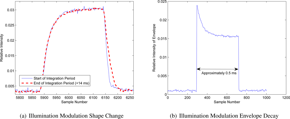
Section 3.3 discussed changes in the correlation waveform over large timescales, primarily due to temperature changes. However, this effect is not limited to long-periods of time; in some systems the modulation waveform shape changes within the integration period. For example, Figure 3(a) presents a comparison between the illumination waveform shape at the beginning and end of a 14 millisecond integration period for the SR-4000. By the end of the integration period, the waveform has increased in width. A similar plot of the envelope of the illumination for a much shorter integration period is given in Figure 3. There are several possible contributors to this effect, including the draining of capacitors in the power supply and temperature changes. As the LEDs and the driving circuitry heat up over the integration period, the overall output intensity drops. The temperature then drops in the interval between integration periods, during which most systems disable the illumination to reduce power consumption.
While previous research [11,13,18,28,34] has noted that the phase linearity response is a function of integration time, no mechanism has been posited to explain this. It appears that the mechanism is most probably due to the variation in illumination output, and possibly similar changes in sensor response. From a calibration perspective this is very problematic because, unless the variation has a simple parametisation, the size of the lookup table or B-spline model required to fully model the spatial, temporal and temperature related variation in phase and amplitude is seriously prohibitive.
What is not immediately obvious is how this small-scale variation in illumination output can result in uneven phase steps. Given a continuously operating system taking measurements of phase steps at equally-spaced intervals with no pauses between subsequent measurements the changes in waveform shape and modulation envelope should be identical across all of the phase steps, thus it would be adequate to merely determine the mean waveform shape over the integration period to calibrate the results. However, if the system is not continuously running, then it is possible for the first phase step to have different behaviour than the rest. This could potentially occur if captures are being triggered in hardware or software, or if all the phase steps are being accumulated and then synchronously read-out together at the end of the phase step sequence. Because the changes in waveform shape are relative small, for short integration times the change in modulation envelope is probably the biggest factor. In this circumstance, the sampling function might be modelled as
where a1, a2 ...am−1 = 1 and a0 ≠ 1. Immediately, the frequency response of the sampling function has changed. Whereas for ideal sampling only harmonics satisfying N + 1 = km resulted in perturbations, perturbing the first phase step makes the sampling function more broadband, allowing other spatial frequencies in the correlation waveform to influence complex domain measurements. A similar model is appropriate for modelling a mismatch between storage regions within each pixel.
Crosstalk is a more complicated electrical phenomenon. All AMCW lidar systems require illumination and sensor modulation signals, while some sensors also have complicated drive signals, such as illumination ‘kicker’ pulses to improve switching times and give more control over the resulting illumination waveform shape. It is tremendously difficult to prevent any leakage of one signal into another, particularly when both the illumination and sensor modulation signals are driving relatively heavy loads from the same power supply in close physical proximity. Our own custom-designed system suffered issues with crosstalk between modulation signals and the readout clock of a CCD camera [35].
Crosstalk is difficult to model as the convolution of a sampling function with a correlation waveform because there strictly is no fixed correlation waveform: effectively, crosstalk results in a correlation waveform shape which is a function of the phase step. While Equation (16) states that frequencies have to be present in both the sampling function and the correlation waveform in order to result in perturbations, crosstalk can theoretically result in the formation of perturbations irrespective of the frequency content of the correlation waveform at any single phase step.
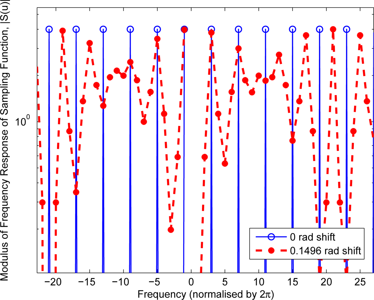
Without detailed knowledge of the inner workings of a particular camera it is difficult to accurately model the crosstalk process, however we can approximate the simplest possible case: that of a perfectly sinusoidal waveform for both the illumination and sensor modulation. In this case crosstalk between the illumination and sensor modulation manifests as a phase and amplitude shift in the modulation. Considering only the case where the illumination signal is perturbing the sensor modulation, the sampling function is then
where ϕi ≈ 0 correspond to the phase shift error in each phase step and ai ≈ 1 correspond to the amplitude of each phase step. Figure 4 demonstrates that shifting just an individual phase step results in sensitivity to all the harmonics of the correlation waveform. In almost all circumstances the positive fundamental is non-zero; thus via Equation (16), the positive fundamental results in a two cycle error in measured phase and amplitude. In general, this two cycle error is the most obvious characteristic of irregular phase sampling. It is interesting to note that exactly the same sort of error is produced by pure axial motion during a frame capture, albeit the inverse squared radial drop-off makes the relationship more complicated. However, if the object is multiple ambiguity distances from the camera then the change in phase step spacing is the biggest effect. The motion problem could potentially be modelled as a type of irregular phase step sampling combined with heterodyning (discussed in Section 4.1).
Figure 1 showed the phase and amplitude response of the Canesta XZ-422 at 44 MHz with an illumination modulation duty cycle of 50% whereas Figure 5(a) shows the phase response if the moduation duty cycle is reduced to 29%, in order to deliberately cancel out the most important perturbing harmonics. Whereas shifting the offset of the illumination waveform in Figure 1 resulted in the aliasing induced error being largely translated, in Figure 5(a) the phase error completely changes depending on the relative phase of the illumination. This is highly indicative of crosstalk. Figure 5(b) shows the results of fitting different models to one of the linearity plots. Assuming even phase sampling and the presence of a fundamental and fifth harmonic, it is impossible to adequately fit the error shape. Using Equation (21) and assuming that the modulation waveforms were pure sinusoids produced a two cycle error which roughly fit the data. Applying the same model by assuming the presence of both a fundamental and fifth harmonic resulted in a near perfect fit. Admittedly, this is based on an extremely naïve model, but attempting to fit a strictly correct model would have too many parameters and overfit the waveform. However, it does demonstrate that irregular phase steps are a plausible mechanism for generating phase and amplitude errors that are not multiples of the number of phase steps.
It is quite difficult to identify whether similar errors are present in other published results because full-information is not always provided, for example, plotting phase error against range without specifying the modulation frequency [8]. Some papers appear to arbitrarily calibrate for all apparent linearity errors (e.g., [16]); without considering the cause, this could potentially lead to the calibration being unknowingly invalidated. Other papers, which only fit parameters which have a known theoretical basis, have ignored a frequency of two completely (e.g., [36]). However, at least one other work has demonstrated a phase error with a frequency of two [37]. Measurements were made using the PMD-19k, SR-3000 and O3D sensors; the PMD-19k and SwissRanger systems were found to have errors with a frequency of four, while the O3D system had errors composed of the sum of frequencies of two and four. Given that all the systems used four samples, the frequencies of four were clearly due to aliasing of the third and fifth harmonics whereas the only plausible explanation for the error of frequency two is irregular phase steps.
3.5. Mixed Pixels/Multipath Interference
Mixed pixels occur around the edges of objects when a single pixel integrates light from more than one backscattering source, often resulting in highly erroneous phase and amplitude measurements. Multipath interference is the same effect but due to scattering either within the camera itself or reflections within a scene. In particular, these effects correspond to a violation of the assumption that there is only a single backscattering source within each pixel. One particularly frustrating scenario is that objects outside the field of view of the camera can result in scattered light. While a number of different restoration approaches have been posited [7,33,38,39], this is still an active area of research.
It is important to be able to identify multipath interference in phase and amplitude response measurements, so that linearity calibrations do not accidentally calibrate for transient phenomena. Assuming a scattering source at a distance ds, with an relative amplitude of b, the complex domain measurement as a function of true range, dξ, can be modelled as
where the brightness of the primary return is assumed to decay according to the inverse squared law. This is equivalent to modelling a fixed scattering source causing errors in a linearity calibration using a translation table.
Figure 6 shows the phase and amplitude perturbations introduced by the multipath interference using b ∈ {0.01, 0.02, 0.05, 0.1} and ds = 0.5. The multipath results in a roughly single cycle error, but with an additional caveat that the two ends of the ambiguity range no-longer match up. If the the change in brightness of the primary return is not modelled, then the error is a single cycle sinusoid. In general, either of these possibilities is quite easily recognised in a plot of phase and amplitude response.
3.6. Systematic Errors from Non-Circularly-Symmetric Noise
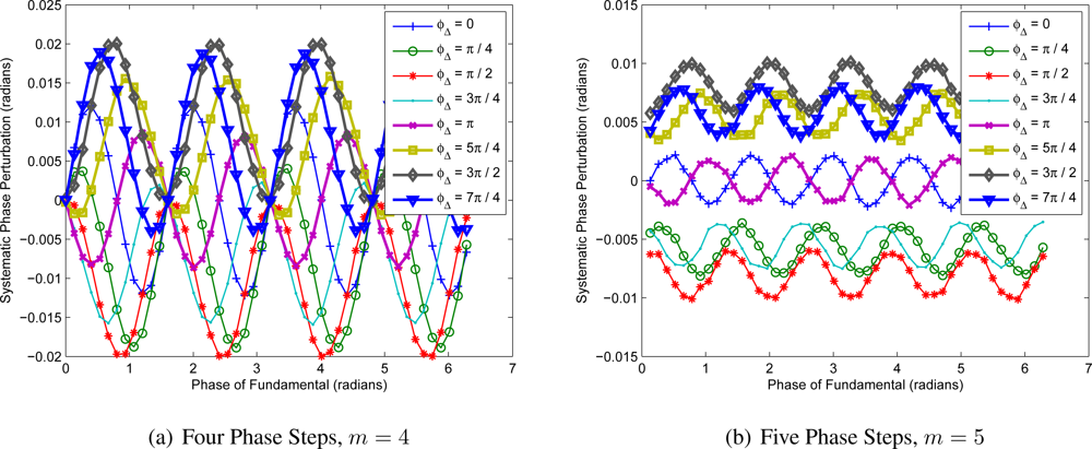
Non-circularly-symmetric noise occurs when the covariance of the real and imaginary parts of a complex domain range measurement is not a scaled identity matrix. Averaging amplitude and phase, rather than averaging complex domain measurements, appears to be a relatively common practice. This averaging method causes overestimation of amplitude and systematic phase perturbations if the noise distribution of the complex domain measurement is not circularly symmetric, although previous studies [40] have assumed circular symmetry. These asymmetric noise distributions occur in the case of non-differential or unbalanced differential measurements where the correlation waveform contains a second harmonic, due to shot noise statistics [33]. All other frequency content contributes circularly symmetric noise. Unfortunately, because the noise distribution is a function of the amount of ambient light integrated by the sensor, it is not possible to calibrate for this systematic phase and amplitude perturbation without extra information. An example is given in Figure 7, where the ith measurement of the correlation waveform is given by
where α = β = 100 photons, m is the number of phase steps, ϕf is the phase delay in the correlation waveform and ϕΔ is the relative phase of the second harmonic. For greater than five phase steps, the characteristics are most similar to Figure 7(b).
A summary of all the perturbation sources and mitigation techniques covered in this section is given in Table 1.
4. Advanced Aliasing Mitigation Methods
In Section 3.2 we discussed standard approaches to mitigating non-linear phase and amplitude responses. However many of the assumptions implicit in these models, such as stable temperatures, do not hold in practice. Rather than trying to calibrate out non-linear phase and amplitude responses after-the-fact, an alternative approach is to use different measurements techniques which change the sampling function so as to remove most of the amplitude and phase errors from aliasing. This section discusses two such methods: heterodyning and harmonic cancellation. Not only do these methods attenuate aliasing harmonics in the equi-sampled case, but they also attenuate harmonics in the case of irregular phase steps, which makes these methods potentially applicable to mitigation of effects such as crosstalk.
4.1. Heterodyning
An alternative to discrete phase stepping is to integrate over a range of relative phases, also known as heterodyning [41]. This can be achieved practically with a small frequency offset between the sensor and illumination modulation signals, resulting in a beating waveform being sampled by the sensor; this beat waveform is essentially equivalent to the standard correlation waveform. If the modulation is free-running, the frequency difference must be equal to the frame rate divided by m to ensure the relative phase sweeps exactly 360 degrees over the sample frames.
With changing phase during integration, the correlation waveform is sampled over a period as
where τ is the integration time as fraction of the allocated sample time, normally slightly less than 1. Although it is desirable for τ to approach 1, the practical limitations of sensor readout time with a continuously operating modulation signal means τ can never reach 1. As τ approaches zero, the heterodyne case approaches the homodyne case.
The sampling function then becomes a series of rectangular functions rather than Dirac deltas, giving
The Fourier transform of this sampling function can be expressed in terms of the homodyne case from Equation (12), giving
follows a sinc function, meaning the harmonics are attenuated compared to the Homodyne case. Therefore, any harmonics aliased onto the negative fundamental will cause less perturbation. Even though this approach will ameliorate linearity errors to some degree, it is not capable of eliminating them. One cost is that the fundamental is attenuated as well as the harmonics, although to a much lesser extent. Heterodyning also partially mitigates the effects of higher frequencies in the correlation waveform in the case of uneven phase steps, although it is unable to attenuate the two cycle phase and amplitude perturbation from the positive fundamental.
With more complicated hardware it is possible to reset the signal generators so as to achieve τ > 1 and overlap phase samples. It is possible to design τ so as to move the zeros of the sinc function to deliberately cancel out a particular unwanted frequency [35]. This is one type of harmonic cancellation, a homodyne variation of which is discussed in the next section.
4.2. Harmonic Cancellation
One of the major constraining factors for real-time operation of an AMCW system is read-out time; as the number of explicit phase steps increases, the overall range measurement frame-rate decreases. An alternative approach is to retain four separate measurements, but integrate over more than one phase step in order to deliberately cancel out the aliasing harmonics. While a true heterodyne approach requires specialised hardware, it is possible to achieve a similar outcome using discrete homodyne phase steps. Payne et al. [42] demonstrated a method using 45 degree phase steps, the xth explicit measurement is composed of sub-measurements at three different phase steps, given by
where the weightings are generally achieved by varying the integration time. Although harmonic cancellation can also be designed to only cancel out certain specific frequencies, in the most general case it operates by simulating a sinusoidal modulation signal. Each sub-measurement is chosen and weighted so that the mean modulation waveform over the entire integration period is as close to sinusoidal as possible; this provides the benefits of a near-sinusoidal modulation signal, although it is only necessary for the modulation itself to be rectangular. One possible implementation, with m underlying phase steps, where m/4 ∈ , is
The technique can easily be generalised to a different number of explicit measurements.
The biggest advantage of harmonic cancellation is that, unlike calibration, it cannot be invalidated by simple changes in the correlation waveform shape due to spatial or temporal variance. The primary limitation of harmonic cancellation is the decreased efficiency of the measurements: if you use eight explicit phase steps, most steps contribute to both the real and imaginary parts of the resultant measurement. In the case of eight step harmonic cancellation with four explicit measurements, each sub-measurement contributes to either the real or imaginary part of the resultant measurement. This requires the repetition of some phase steps, which eight explicit phase steps does not require. However, because most systems are accuracy limited and not precision limited, harmonic cancellation is generally of net benefit.
The sampling function in the case of harmonic cancellation with m underlying phase steps is given in Equation (12), ignoring the impacts of integration time. In other words, the phase and amplitude response are identical to the eight explicit phase step case, thus the third harmonic no-longer aliases onto the fundamental.
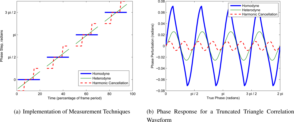
An example of the impact of heterodyning and harmonic cancellation is given in Figure 8. In theory, a perfect lookup table or B-spline model could fully model this non-linearity producing a flat response; unfortunately, no such perfect model is possible in practice. The truncated triangle waveform corresponds to the convolution of 25% duty cycle rectangular modulation with 62.5% duty cycle rectangular modulation. The heterodyne modulation was assumed to have τ = 0.8. Harmonic cancellation is shown to produce the least phase error, followed by the heterodyne approach.
5. Conclusions
In this paper we have reviewed the literature on non-linear phase and amplitude responses and developed a detailed model for the measurement and sampling process inherent to AMCW lidar. Using this model it was shown how the aliasing of correlation waveform harmonics impacts on phase and amplitude response and how standard amelioration techniques such as lookup tables and B-spline models can be invalidated by subtle effects such as temperature changes. Real data was presented showing how phase and amplitude changes temporally and spatially across a full-field CMOS sensor. The mixed pixel and multipath interference problems were demonstrated to cause a roughly single cycle error over 2π radians, although frequently the measurements at zero and 2π do not match up perfectly. Other phenomena were identified that do not appear to have been previously discussed in the literature: these effects included changes in modulation waveform shape over an integration period, changes in the overall intensity envelope of the modulation and crosstalk between modulation signals. It was shown that these error sources result in irregular phase steps, generally manifesting as two cycle errors over a full 2π phase sweep, a type of error that the aliasing of correlation waveform harmonics is unable to cause. It was also demonstrated that non-circularly-symmetric noise statistics, caused by the presence of a second harmonic in the correlation waveform, are capable of producing systematic phase errors in the case of non-differential or unbalanced differential measurements. Finally, heterodyning and harmonic cancellation were considered as partial solutions to non-linearity issues in practical systems. It was shown that harmonic cancellation provides a significant improvement in phase and amplitude linearity.
Acknowledgments
A big thank-you to Andrew Payne for allowing us to use some of his experimental data in this paper. This research was supported by the University of Waikato Strategic Investment Fund.
References
- Xu, Z.; Heinol, H.G.; Schwarte, R.; Loffeld, O. An enhanced multi-probing recovering algorithm based on color mixed nonlinear modulation and its application in a 3D vision system. Proc. SPIE 1995, 2588, 200–207. [Google Scholar]
- Lange, R. 3D Time-Of-Flight Distance Measurement with Custom Solid-State Image Sensors in CMOS/CCD-Technology. Ph.D. Thesis, University of Siegen, Siegen, Germany. 2000. [Google Scholar]
- Luan, X. Experimental Investigation of Photonic Mixer Device and Development of TOF 3D Ranging Systems Based on PMD Technology. Ph.D. thesis, University of Siegen, Siegen, Germany. 2001. [Google Scholar]
- Hussmann, S.; Edeler, T. Performance Improvement of a 3D-TOF PMD Camera Using a Pseudo 4-Phase Shift Algorithm. Proceedings of IEEE Instrumentation and Measurement Technology Conference, Singapore, 5–7 May 2009; pp. 542–546.
- Schmidt, M.; Zimmermann, K.; Jahne, B. High Frame Rate for 3D Time-Of-Flight Cameras by Dynamic Sensor Calibration. Proceedings of IEEE International Conference on Computational Photography, Pittsburgh, PA, USA, 8–10 April 2011.
- Godbaz, J.P.; Cree, M.J.; Dorrington, A.A. Multiple return separation for a full-field ranger via continuous waveform modelling. Proc. SPIE 2009, 7251, 72510T. [Google Scholar]
- Godbaz, J.P.; Cree, M.J.; Dorrington, A.A. Mixed Pixel Return Separation for a Full-Field Ranger. Proceedings of Image and Vision Computing New Zealand 2008 (IVCNZ’08), Lincoln, New Zealand, 26–28 November 2008; pp. 1–6.
- Lindner, M.; Kolb, A.; Ringbeck, T. New Insights into the Calibration of ToF-Sensors. Proceedings of IEEE Computer Vision and Pattern Recognition Workshop, Anchorage, AK, USA, 23–28 June 2008; pp. 1–5.
- Kang, B.; Kim, S.J.; Lee, S.; Lee, K.; Kim, J.D.K.; Kim, C.Y. Harmonic distortion free distance estimation in ToF camera. Proc. SPIE 2011, 7864, 786403. [Google Scholar]
- Kahlmann, T.; Ingensand, H. Calibration and improvements of the high-resolution range-imaging camera SwissRanger. Proc. SPIE 2005, 5665, 144–155. [Google Scholar]
- Kahlmann, T.; Remondino, F.; Ingensand, H. Calibration for Increased Accuracy of the Range Imaging Camera SwissRanger. Proceedings of ISPRS Commission V Symposium ‘Image Engineering and Vision Metrology’, Dresden, Germany, 25–27 September 2006.
- Lindner, M.; Kolb, A. Lateral and depth calibration of PMD-distance sensors. In Advances in Visual Computing; Lecture Notes in Computer Science; Springer: Berlin/Heidelberg, Germany, 2006; Volume 4292, pp. 524–533. [Google Scholar]
- Lindner, M.; Kolb, A. Calibration of the intensity-related distance error of the PMD TOF-camera. Proc. SPIE 2007, 6764, 67640W. [Google Scholar]
- Lichti, D.D. Self-calibration of a 3D range camera. In The International Archives of the Photogrammetry, Remote Sensing and Spatial Information Sciences; ISPRS: Vienna, Austria, 2008; Volume 37, Part B5; pp. 1–6. [Google Scholar]
- Rapp, H.; Frank, M.; Hamprecht, F.A.; Jahne, B. A theoretical and experimental investigation of the systematic errors and statistical uncertainties of Time-Of-Flight cameras. Int. J. Intell. Syst. Technol. Appl 2008, 5, 402–413. [Google Scholar]
- Fuchs, S.; Hirzinger, G. Extrinsic and Depth Calibration of TOF Cameras. Proceedings of IEEE Conference on Computer Vision and Pattern Recognition, CVPR 2008, Anchorage, AK, USA, 23–28 June 2008.
- Keller, M.; Kolb, A. Real-time simulation of time-of-flight sensors. Simul. Model. Pract. Th 2009, 17, 967–978. [Google Scholar]
- Schmidt, M.; J¨ahne, B. A Physical Model of Time-of-Flight 3D Imaging Systems, Including Suppression of Ambient Light. Proceedings of Dyn3D ’09 The DAGM 2009 Workshop on Dynamic 3D Imaging, Jena, Germany, 9 September 2009; Springer-Verlag: Berlin/Heidelberg, Germany, 2008; 5742, pp. 1–15. [Google Scholar]
- Lindner, M.; Schiller, I.; Kolb, A.; Koch, R. Time-of-Flight sensor calibration for accurate range sensing. Comput. Vis. Image Underst 2010, 114, 1318–1328. [Google Scholar]
- Foix, S.; Alenya, G.; Torras, C. Lock-in Time-of-Flight (ToF) cameras: A survey. IEEE Sens. J 2011, 11, 1917–1926. [Google Scholar]
- Payne, A.D.; Dorrington, A.A.; Cree, M.J. Illumination waveform optimization for Time-of-Flight range imaging cameras. Proc. SPIE 2011, 8085, 80850D. [Google Scholar]
- Fuchs, S.; May, S. Calibration and Registration for precise surface reconstruction with TOF cameras. Int. J. Intell. Syst. Technol. Appl 2008, 5, 274–284. [Google Scholar]
- Abdo, N.; Borgeat, A. 3D Camera Calibration; Technical Report; Albert-Ludwigs-University Freiburg: Freiburg, Germany, 2010. [Google Scholar]
- Payne, A.D.; Dorrington, A.A.; Cree, M.J.; Carnegie, D.A. Characterizing an image intensifier in a full-field range imaging system. IEEE Sens. J 2008, 8, 1763–1770. [Google Scholar]
- Richardson, W.H. Bayesian-based iterative method of image restoration. J. Opt. Soc. Amer 1972, 62, 55–59. [Google Scholar]
- Lucy, L.B. An iterative technique for the rectification of observed distributions. Astronom. J 1974, 79, 745. [Google Scholar]
- Kahlmann, T.; Ingensand, H. Calibration of the fast range imaging camera SwissRanger for use in the surveillance of the environment. Proc. SPIE 2006, 6396, 639605. [Google Scholar]
- Steiger, O.; Felder, J.; Weiss, S. Calibration of Time-of-Flight Range Imaging Cameras. Proceedings of 15th IEEE International Conference on Image Processing, San Diego, CA, USA, 12–15 October 2008; pp. 1968–1971.
- Chiabrando, F.; Chiabrando, R.; Piatti, D.; Rinaudo, F. Sensors for 3D imaging: Metric evaluation and calibration of a CCD/CMOS Time-of-Flight camera. Sensors 2009, 9, 10080–10096. [Google Scholar]
- Karel, W. Integrated range camera calibration using image sequences from hand-held operation. In The International Achives of the Photogrammetry, Remote Sensing and Spatial Information Sciences; ISPRS: Vienna, Austria, 2008; Volume 37, Part B5. [Google Scholar]
- Kahlmann, T.; Ingensand, H. High-precision investigations of the fast range imaging camera SwissRanger. Proc. SPIE 2007, 6758, 67580J. [Google Scholar]
- Boehm, J.; Pattinson, T. Accuracy of exterior orientation for a range camera. In The International Archives of the Photogrammetry, Remote Sensing and Spatial Information Sciences; ISPRS: Vienna, Austria, 2010; Volume 38, Part 5. [Google Scholar]
- Godbaz, J.P. Ameliorating Systematic Errors in Full-Field AMCW Lidar. Ph.D. Thesis, The University of Waikato, Waikato, New Zealand. 2011. [Google Scholar]
- Radmer, J.; Fust, P.M.; Schmidt, H.; Krger, J. Incident Light Related Distance Error Study and Calibration of the PMD-Range Imaging Camera. Proceedings of IEEE Computer Society Conference on Computer Vision and Pattern Recognition Workshops, Anchorage, AK, USA, 24–26 June 2008.
- Payne, A.D. Development of a Full-Field Time-of-Flight Range Imaging System. Ph.D. Thesis, The University of Waikato, Waikato, New Zealand. 2008. [Google Scholar]
- Lichti, D.D. Error modelling, calibration and analysis of an AM-CW terrestrial laser scanner system. ISPRS J. Photogramm 2007, 61, 307–324. [Google Scholar]
- Rapp, H. Experimental and Theoretical Investigation of Correlating TOF-Camera Systems. Ph.D. Thesis, University of Heidelberg, Heidelberg, Germany. 2007. [Google Scholar]
- Dorrington, A.A.; Godbaz, J.P.; Cree, M.J.; Payne, A.D.; Streeter, L.V. Separating true range measurements from multi-path and scattering interference in commercial range cameras. Proc. SPIE 2011, 7864, 786404. [Google Scholar]
- Mure-Dubois, J.; Hügli, H. Optimized scattering compensation for Time-of-Flight camera. Proc. SPIE 2007, 6762, 67620H. [Google Scholar]
- Frank, M.; Plaue, M.; Rapp, H.; Köthe, U.; J¨ahne, B.; Hamprecht, F.A. Theoretical and experimental error analysis of continuous-wave time-of-flight range cameras. Opt. Eng 2009, 48, 013602. [Google Scholar]
- Dorrington, A.A.; Cree, M.J.; Payne, A.D.; Conroy, R.M.; Carnegie, D.A. Achieving sub-millimetre precision with a solid-state full-field heterodyning range imaging camera. Meas. Sci. Tech 2007, 18, 2809–2816. [Google Scholar]
- Payne, A.D.; Dorrington, A.A.; Cree, M.J.; Carnegie, D.A. Improved linearity using harmonic error rejection in a full-field range imaging system. Proc. SPIE 2008, 6805, 68050D. [Google Scholar]
Figure 1.
The phase error and amplitude response of a Canesta XZ-422 system operating at 44 MHz with a 50% illumination modulation duty cycle as a function of relative phase of the illumination modulation. The majority of the systematic error is due to aliasing of the positive third harmonic.
Figure 1.
The phase error and amplitude response of a Canesta XZ-422 system operating at 44 MHz with a 50% illumination modulation duty cycle as a function of relative phase of the illumination modulation. The majority of the systematic error is due to aliasing of the positive third harmonic.
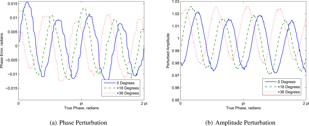
Figure 2.
Spatial and long-period temporal variation in the reference waveform shape for a modulated CMOS sensor.
Figure 2.
Spatial and long-period temporal variation in the reference waveform shape for a modulated CMOS sensor.
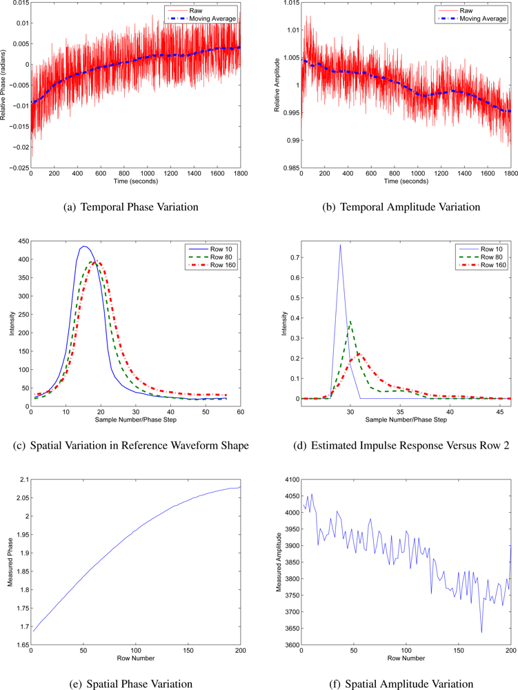
Figure 3.
Variation in SwissRanger 4000 illumination modulation waveform shape within a single integration period.
Figure 3.
Variation in SwissRanger 4000 illumination modulation waveform shape within a single integration period.

Figure 4.
Frequency content of the sampling function using the crosstalk model of Equation (21), for ai=1, ϕ0=ϕ2=0 and ϕ1=–ϕ3 as a function of phase shift, ϕ1.
Figure 4.
Frequency content of the sampling function using the crosstalk model of Equation (21), for ai=1, ϕ0=ϕ2=0 and ϕ1=–ϕ3 as a function of phase shift, ϕ1.

Figure 5.
The phase and amplitude response of a Canesta XZ-422 system operating at 44 MHz with a 29% illumination modulation duty cycle as a function of relative phase of the illumination modulation. Only a portion of the remaining error is due to aliasing.
Figure 5.
The phase and amplitude response of a Canesta XZ-422 system operating at 44 MHz with a 29% illumination modulation duty cycle as a function of relative phase of the illumination modulation. Only a portion of the remaining error is due to aliasing.
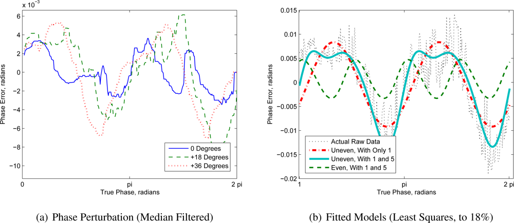
Figure 6.
Simulation of the impact of scattered light on phase and amplitude response.
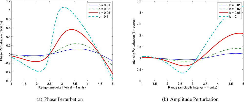
Figure 7.
Simulation of the systematic perturbation introduced by non-circularly symmetric error in the complex domain measurement as a function of the phase shift in the correlation waveform, ϕf.
Figure 7.
Simulation of the systematic perturbation introduced by non-circularly symmetric error in the complex domain measurement as a function of the phase shift in the correlation waveform, ϕf.

Figure 8.
Evaluating Advanced Aliasing Mitigation Methods.


| Perturbation Source | Error Nature in Cycles/2π (using translation stage) | Countermeasures |
|---|---|---|
| Aliasing | km cycle error | Adjust modulation duty cycles Calibration (lookup tables/B-splines) Heterodyning (see Section 4) Harmonic cancellation (see Section 4) |
| Crosstalk Modulation envelope changes | Prominent 2 cycle error, any additional cyclic error | Hardware redesign Heterodyning Harmonic cancellation |
| Mixed pixels Multipath interference | Roughly one cycle error, ends may not match up | Mixed pixel restoration algorithms Anti-reflection lens coatings |
| Non-circularly-symmetric noise | m cycle error | Average complex measurements Adjust modulation duty cycles Differential sampling Ensure A and B channels are matched |
| Temporal phase/amplitude drift | Ends do not match up | Hardware redesign Optical feedback |
Share and Cite
MDPI and ACS Style
Godbaz, J.P.; Cree, M.J.; Dorrington, A.A. Understanding and Ameliorating Non-Linear Phase and Amplitude Responses in AMCW Lidar. Remote Sens. 2012, 4, 21-42. https://doi.org/10.3390/rs4010021
AMA Style
Godbaz JP, Cree MJ, Dorrington AA. Understanding and Ameliorating Non-Linear Phase and Amplitude Responses in AMCW Lidar. Remote Sensing. 2012; 4(1):21-42. https://doi.org/10.3390/rs4010021
Chicago/Turabian StyleGodbaz, John P., Michael J. Cree, and Adrian A. Dorrington. 2012. "Understanding and Ameliorating Non-Linear Phase and Amplitude Responses in AMCW Lidar" Remote Sensing 4, no. 1: 21-42. https://doi.org/10.3390/rs4010021