1. Introduction
When a laser beam hits the forest canopy non-vertically, the other side of the canopy objects is partly or totally shadowed and there are areas on the ground receiving no hits or only a small number of hits (shadowing effect). Similarly in urban mapping with airborne laser scanner (ALS), the facades of buildings in built-up environments and ground elevations cannot be obtained from shadowed areas. Thus, shadowing causes problems in the 3-D reconstruction of buildings and trees as well as when determining Digital Terrain/Elevation Models (DTM/DEM). At the time of the advent of airborne laser scanning, the shadowing problem was considered to be a serious challenge. The TopoSys airborne laser scanner was designed to include a scanning angle of ±7.1 degrees off-nadir in order to minimize shadow formation [
1]. Since then, laser scanning has been applied to tasks such as the creation and updating of nationwide elevation models and standwise forest inventories where data covering large areas need to be collected cost-efficiently. Presently, scanning angles of ±15 degrees have been generally accepted in operational work, but larger scanning angles are also applied, e.g., in Finnish and Swedish nationwide airborne laser scanning, the corresponding scanning angle is ±20 degrees.
The accuracy of elevation models and forest inventory products is relatively well known as regards the application of airborne laser scanning in boreal forests [
2,
3,
4,
5,
6,
7], and the associated filtering techniques have been adequately reported (e.g., [
8,
9]). The works of Reutebuch
et al. [
4] and Hyyppä
et al. [
10] can be recommended as overviews of the elevation model’s accuracy. Using TopEye MK I laser scanner data with 4 pulses per m
2, Reutebuch
et al. [
4] reported elevation random errors of 14 cm for boreal forest clear-cuts, 14 cm for heavily-thinned forest, 18 cm for lightly-thinned forest, and 29 cm for uncut forest. Variation in ALS-derived DEM quality with respect to date, flight altitude, pulse mode, terrain slope, forest cover, and within-plot variation was reported by Hyyppä
et al. [
10].
Ahokas
et al. [
11] mentioned that the optimization of the scanning angle (
i.e., field of view) is an important part of nationwide airborne laser scanning. Significant savings in flying time (and thus in costs) can be achieved by increasing the scanning angle and flight altitude. The initial results obtained using scanning angle analysis showed that the scanning angle had an impact on the accuracy of DEMs, but that other factors, such as forest density, dominate the process. Scanning angles up to 15 degrees appear to be usable in DEM production in high-altitude laser scanning within the boreal forest zone. High-altitude laser scanning yielded an accuracy of about ±20 cm (std), which is good enough for most terrain models in forested areas. Ahokas
et al. [
11] stressed that the impact of the scanning angle should be studied further for elevation modeling as the maximum field of view of commercial laser scanners can be up to 75 degrees (
i.e., maximum scanning angle up to 37.5 degrees).
Su
et al. [
12] analyzed the influence of vegetation, slope, and the sampling angle in airborne laser scanning (the laser beam angle from nadir) on DEM accuracy. Vegetation was the greatest source of error in the LiDAR (Light Detection And Ranging) -derived elevation model. Closed and semi-open aspen forest had the greatest signed (+) errors and lowland meadows the greatest (−) errors. ALS should be done in early spring or late autumn in order to mitigate the effect of vegetation. It was also reported that DEM accuracy decreased when the slope gradient increased. The off-nadir scanning angles should be less than 15 degrees to minimize the errors introduced by steep slope gradients. The LiDAR sampling angle had little impact on the measured error and it was not important. Holmgren
et al. [
13] simulated the effects of LiDAR scanning angle for the purpose of estimating mean tree height and canopy closure. Simulations revealed that the laser height percentiles and the proportion of canopy returns changed more with an increased scanning angle for long-crowned species like Norway spruce, compared with short-crowned species like Scots pine. Also, the proportion of canopy returns was affected by scanning angle more than the laser height percentiles were. Chasmer
et al. [
5] investigated laser pulse penetration through a conifer canopy by integrating airborne and terrestrial LiDAR. They found that pulses with higher energy penetrated further into the canopy. The authors suggest that future research should concentrate on improving the understanding of how laser-pulse returns are triggered within vegetated environments and how canopy properties influence the location of the trigger event. Morsdorf
et al. [
14] assessed the influence of flying altitude and scanning angle on biophysical vegetation products (tree height, crown width, fractional cover, and leaf area index) derived from airborne laser scanning. Due to the small scanning angle of the TopoSys Falcon II (±7.15 degrees), the dependence of airborne laser scanning on the incidence angle is not so evident. The angle of incidence (the angle to the surface normal of the horizontal plane) appears to be of greater importance for vegetation density parameters than the local angle of incidence (the angle to the surface normal in the elevation model). The local topography is, thus, less important than the scanning angle. ALS data from larger scanning angles should be used to study further the impact of the scanning angle on vegetation density products. Ahokas
et al. [
15] showed that laser-beam transmittance through the canopy of a small group of Norway spruce trees is a non-linear function of biomass based on the results of an indoor experiment. The scanning angle had only a minor impact on the results when compared to changes in the biomass. Scanning angles of up to 38 degrees proved to be feasible for elevation mapping in this indoor experiment. It was proposed that airborne experiments need to be continued in this subject area.
This being so, the present paper tells of research on the transmittance of laser pulses through the forest canopy as a function of forest attributes (inventory parameters) and the scanning angle from the point of view of elevation modeling. Transmittance was defined as the ratio of the number of pulses within a threshold of the detected elevation model to the total number of transmitted pulses. The motivation for the study is in that if the scanning angle impact on transmittance is minor, then a larger scanning angle range can be accepted in future in applications where small shadowed areas can be accepted as long as the average number of ground hits is also acceptable.
3. Results and Discussion
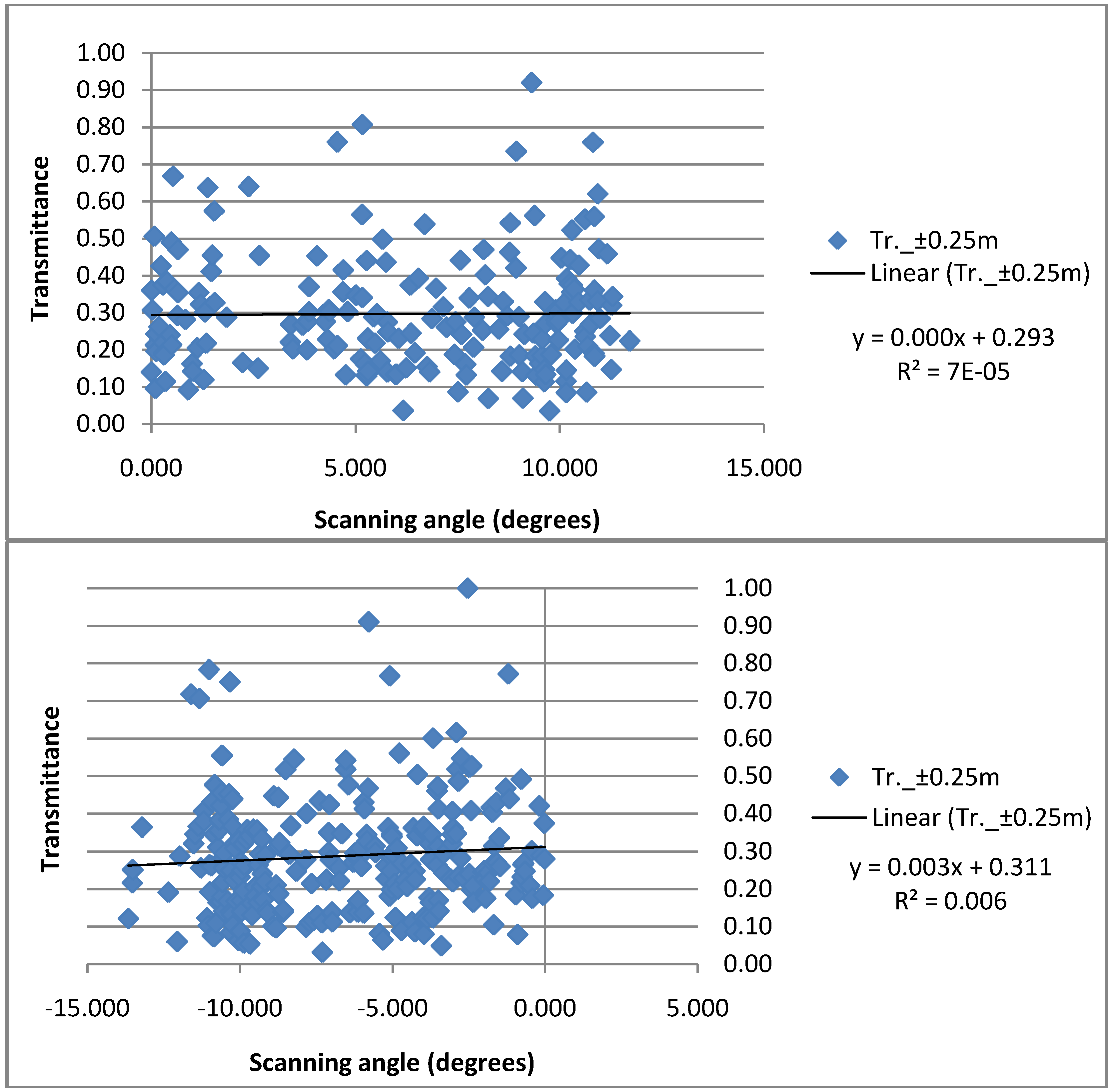
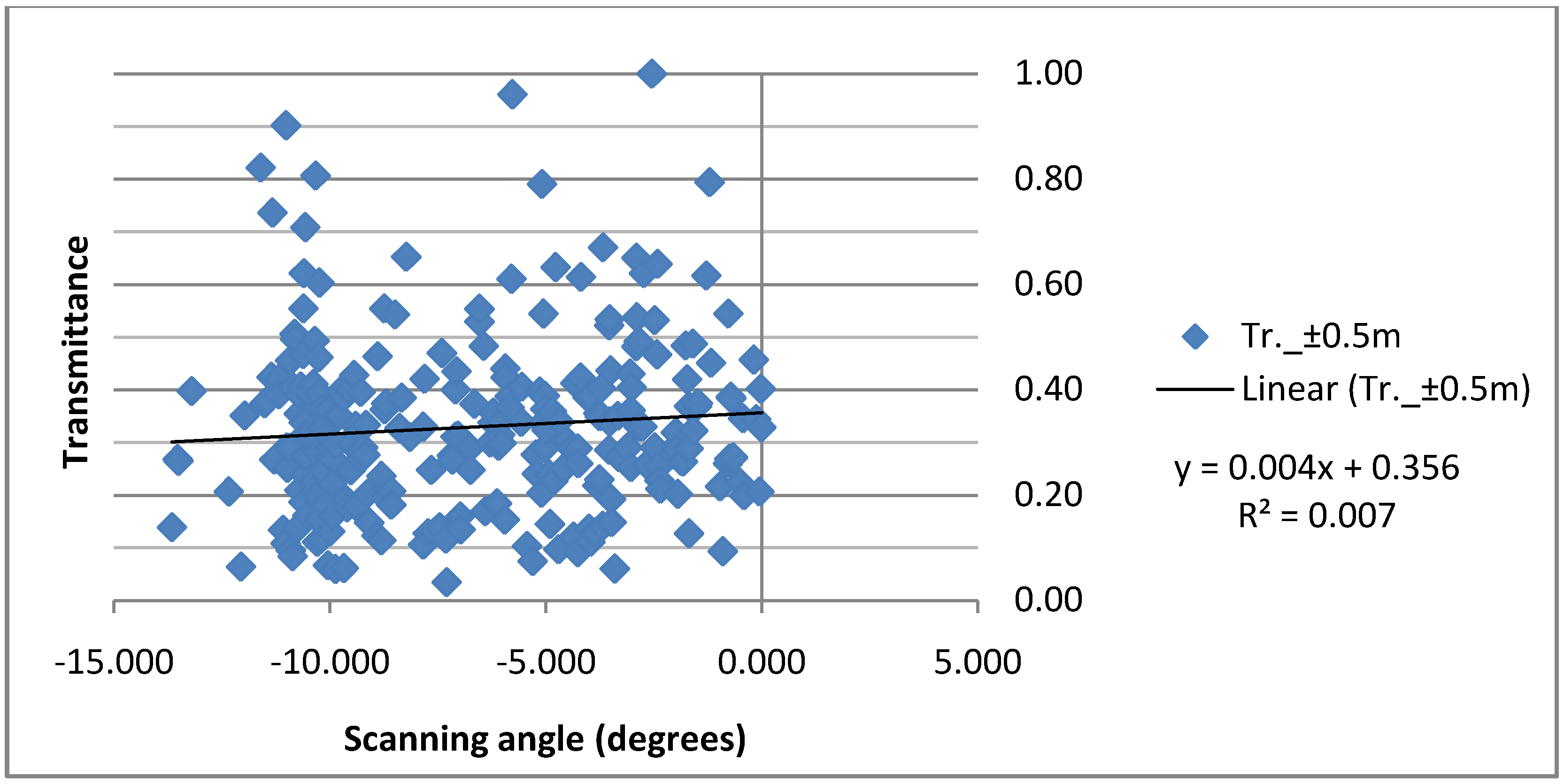
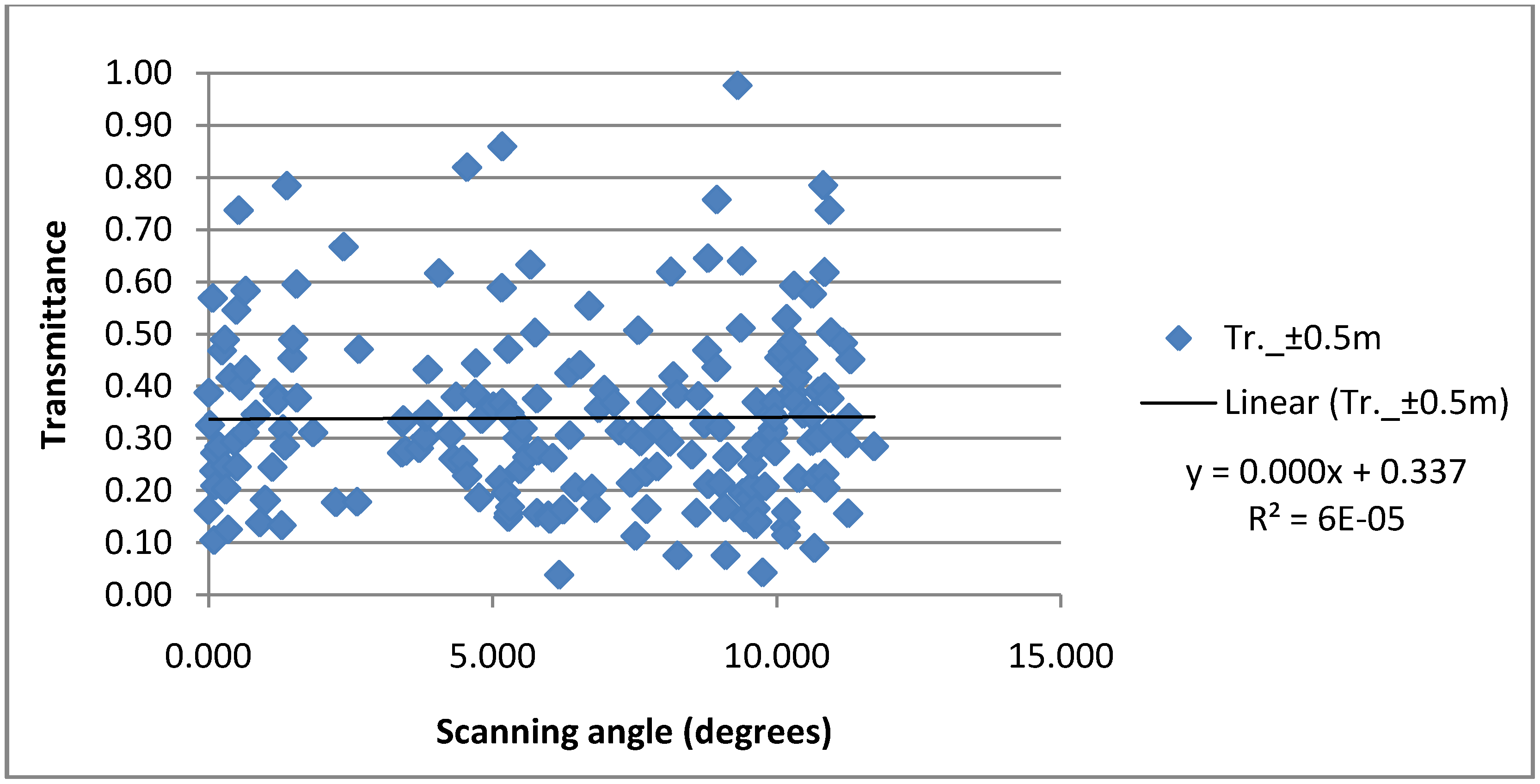
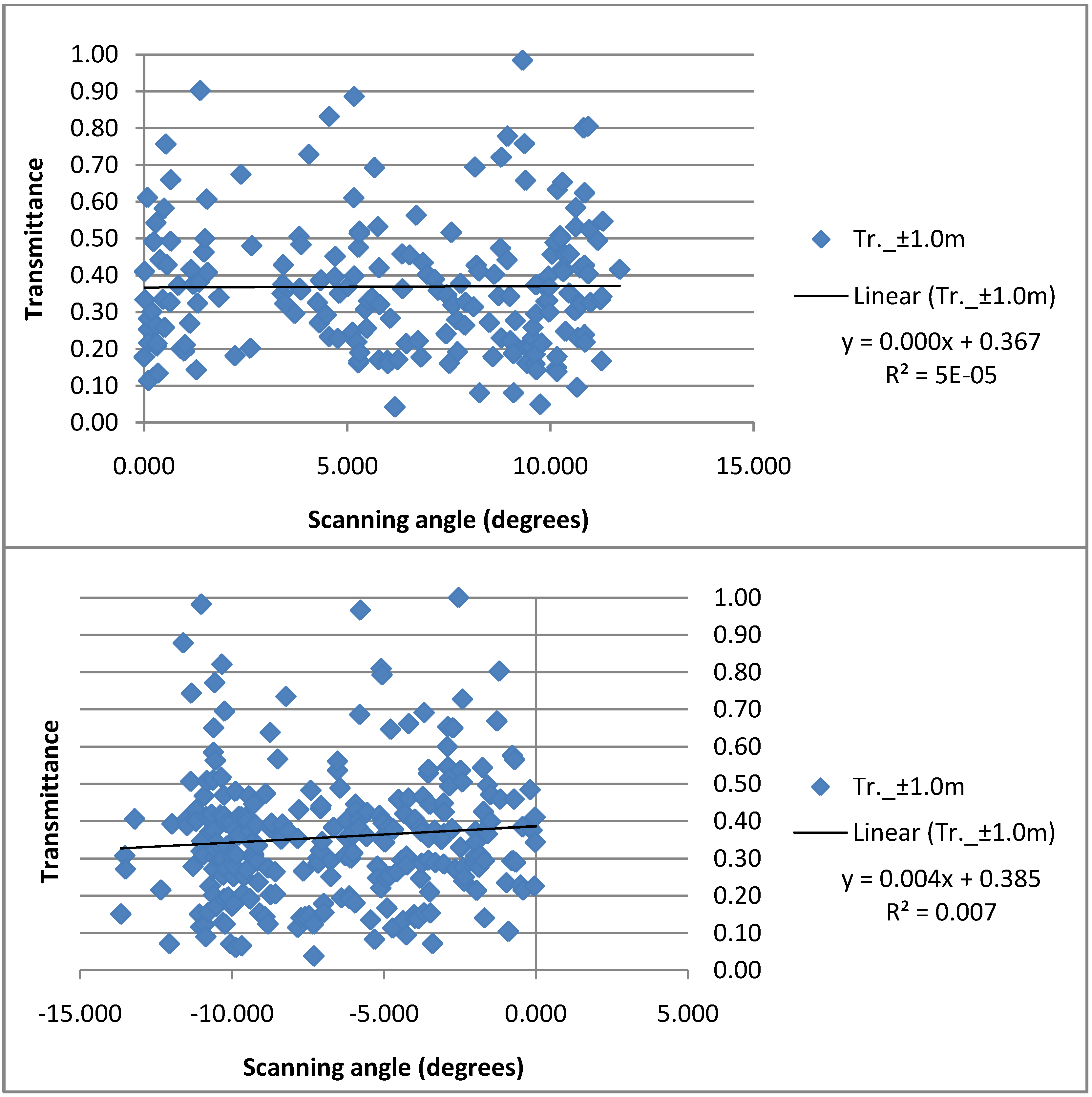
When looking at the relationship between the transmittance and the scanning angle,
Figure 1,
Figure 2 and
Figure 3 depict how the transmittance of laser pulses through the canopy of a boreal forest occurs in relation to the scanning angle. The angles are negative to left of the flight line and positive to the right. As can be seen from the figures and from the coefficients of determination (R
2), which are very small (0.0001 to 0.008), there is basically no correlation between the transmittance and the scanning angle when examining this data set.
Figure 1.
Transmittance scatter of the laser pulses through the canopy of a boreal forest across the scanning angle. Ground tolerance level ±0.25 m.
Figure 1.
Transmittance scatter of the laser pulses through the canopy of a boreal forest across the scanning angle. Ground tolerance level ±0.25 m.
Figure 2.
Transmittance scatter of the laser pulses through the canopy of a boreal forest across the scanning angle. Ground tolerance level ±0.5 m.
Figure 2.
Transmittance scatter of the laser pulses through the canopy of a boreal forest across the scanning angle. Ground tolerance level ±0.5 m.
Figure 3.
Transmittance scatter of the laser pulses through the canopy of a boreal forest across the scanning angle. Ground tolerance level ±1.0 m.
Figure 3.
Transmittance scatter of the laser pulses through the canopy of a boreal forest across the scanning angle. Ground tolerance level ±1.0 m.
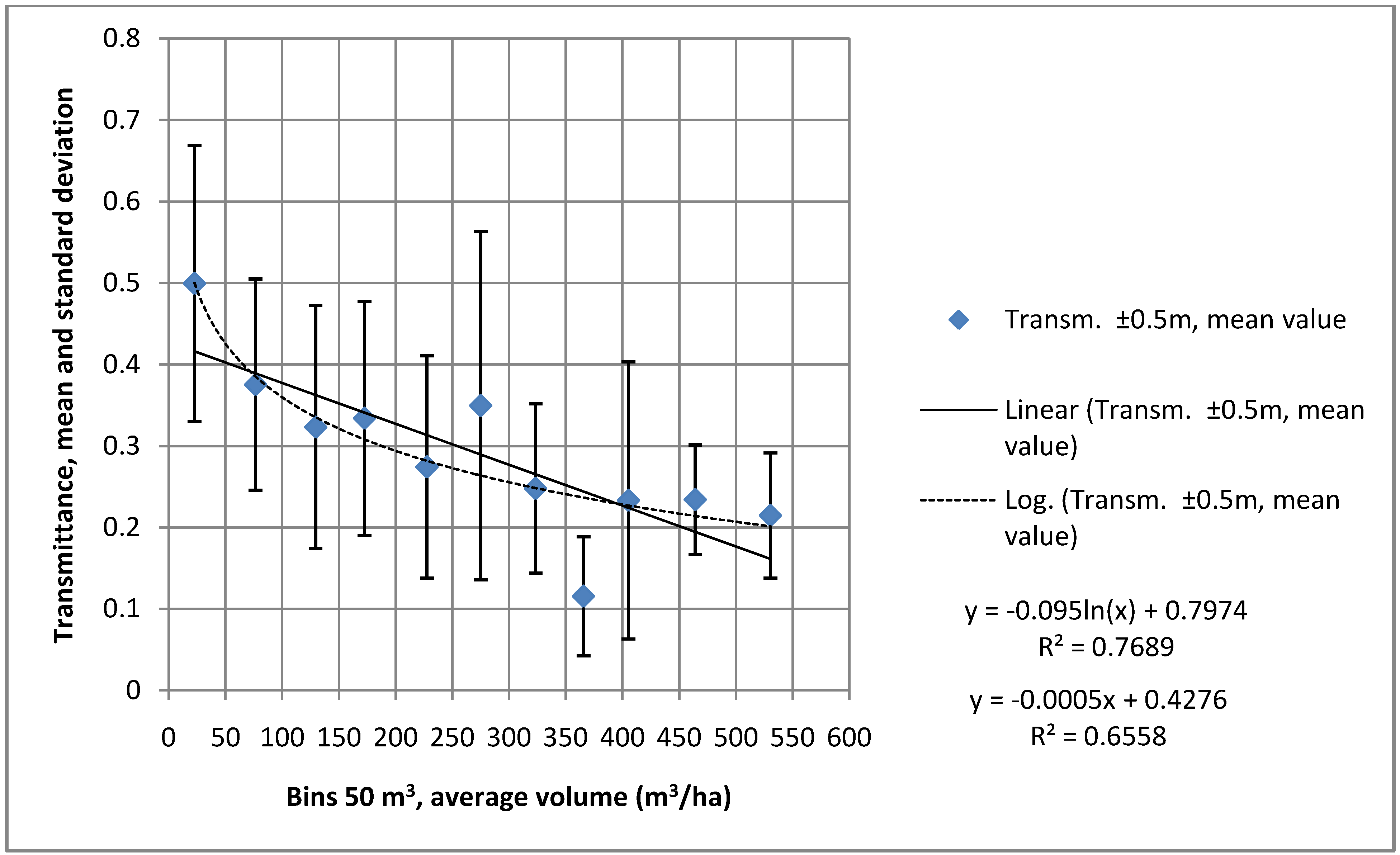
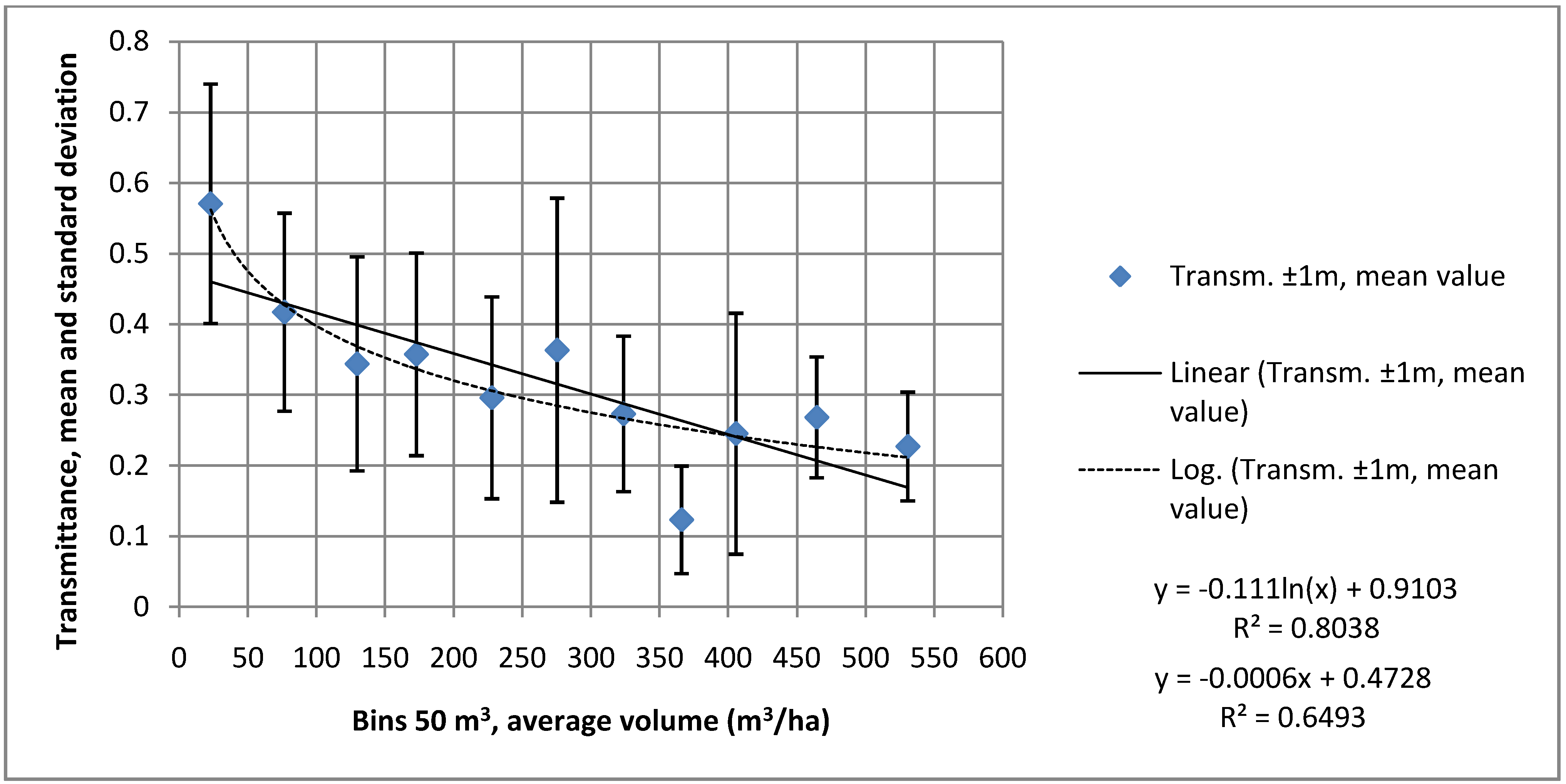
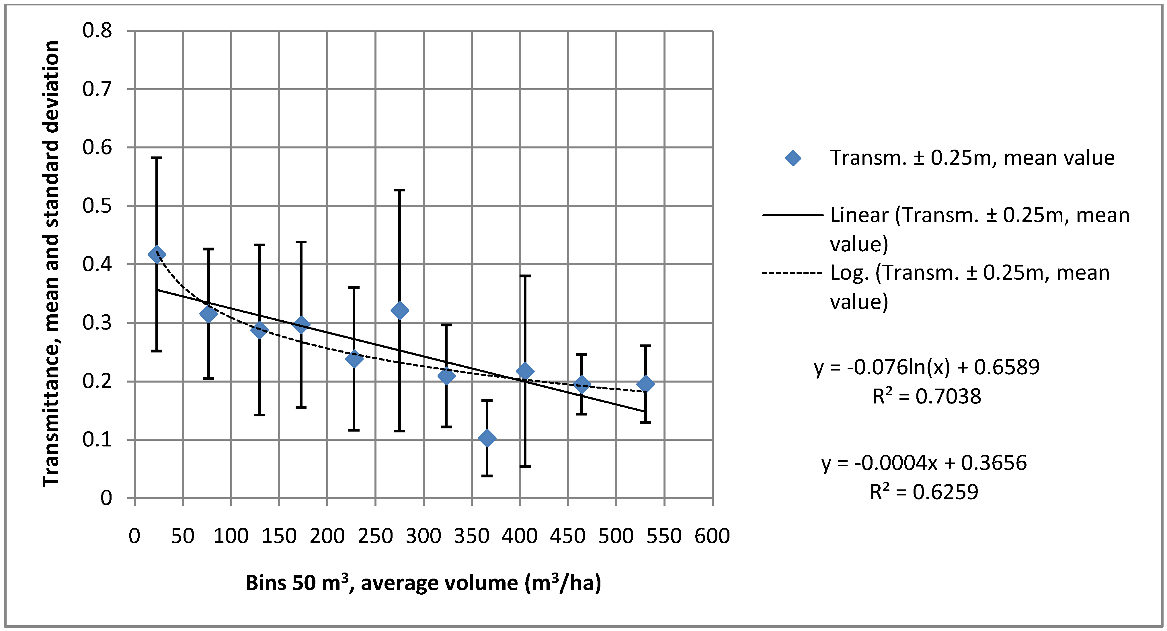
As the scanning angle has only a minor impact on the transmittance of laser pulses through the forest canopy, transmittance was further studied as a function of the stem volume.
Figure 4.
Transmittance through the canopy to the ground as a function of stem volume. Ground tolerance level ±0.25 m.
Figure 4.
Transmittance through the canopy to the ground as a function of stem volume. Ground tolerance level ±0.25 m.
Figure 5.
Transmittance through the canopy to the ground as a function of stem volume. Ground tolerance level ±0.5 m.
Figure 5.
Transmittance through the canopy to the ground as a function of stem volume. Ground tolerance level ±0.5 m.
Figure 6.
Transmittance through the canopy to the ground as a function of stem volume. Ground tolerance level ±1.0 m.
Figure 6.
Transmittance through the canopy to the ground as a function of stem volume. Ground tolerance level ±1.0 m.
The test plot stem volumes were divided into 50 m
3 bins by calculating an average of volumes inside the bin and the mean transmittance for this bin in order to find out the general behavior between these parameters. The results are illustrated in
Figure 4,
Figure 5 and
Figure 6. The logarithmic curve fits better in the data set giving R
2 values 0.70, 0.77, and 0.80, and thus transmittance depends markedly on the stem volume of the trees. The standard deviation of transmittance varies between the bins because the test plots have different characteristics. Some include trees belonging to only one age class while others have trees and tree species belonging to various age classes and tree species. Also, the homogeneity of the forest plots impacts on the results. We assume that lower transmittances may result from plots having multiple stories (various age classes of trees) and from more homogeneous plots. The plots with the greatest heterogeneity and gaps are expected to manifest the highest transmittances. For example, if a plot consists of 50% of gaps and 50% of stem volume of 500 m
3/ha, the transmittance is roughly 0.55 ((1 + 0.2 according to
Figure 4)/2), and average volume is 250 m
3/ha. Since deciduous trees are found mainly in mixed stands, the number of totally closed stands was very small and gaps dominated in the obtained transmittances.
Figure 7 includes pulse transmittances from studies by Næsset [
6,
19] and Solberg
et al. [
20] for comparison. In the paper presented by Næsset [
19], the dates of the laser scannings were 8 June and 9 June 1999, and 6 June 2000, the scan angles were ±14 degrees, the pulse density was about 1.1 per m
2, and the flight height was 700 m. In the study by Næsset [
6], the laser scanning was done on 16 July and 17 July 2001, the flight height was 530–540 m, the average pulse density was 0.84–0.89 per m
2 and pulses transmitted at scan angles greater than 15 degrees were excluded. In the paper presented by Solberg
et al. [
20], the laser scanning was carried out on 26 July 2005, the flight height was 650 m, and pulses transmitted at scan angles greater than 12 degrees were excluded. The mean values of the transmitted pulses were within the range of 4–5.8 per m
2. The vertical line with respect to the mean transmittance shown in the figure is the range of the rate of transmittance through the canopy. The forest area in question had been actively managed, it was distinctly divided into stands of various age classes, and it was dominated mostly by Scots pine with a few stands of Norway spruce and deciduous trees. The use of the first pulse model and possibly the lack of understories, were the reasons for the high transmittance values in the study by Solberg
et al. [
20] when compared to the results of other studies. The data in this study were collected on 25 July 2009 and the scan angles were ±15 degrees. The laser scannings for these studies were conducted when the vegetation was in leaf. In general, the levels of transmittances were high, and the transmittance values could have been even higher as the early spring is the primary season for collecting elevation data.
The scanning angles varied from 12 to 15 degrees. The average pulse density between the studies differed significantly, but that was not believed to affect transmittance. The results also showed that by merging transmittance and volume characteristics from previous studies, the general trend was not visible from them. It is also possible that the definition of transmittance (what points are considered as ground points) varies between studies.
The results of
Figure 7 also show that there are other forest attributes, depicted in
Section 2.4, that impact on transmittance.
Table 2 shows their inter-correlation. Moreover, the canopy structure and LAI (Leaf Area Index) are believed to impact on the results, but it is difficult to compare the results between different studies subject to different circumstances. However, the impact of other predictors on transmittance was modeled further. The basal area had the largest single impact on the transmittance model and the mean angle had the least impact (
Table 3 and
Table 4).
Table 4 summarizes the results of the linear models. LnTr-models fit better than Tr-models.
Figure 7.
Transmittance through the canopy to the ground as a function of stem volume. Comparison of data from this study with the data of three other studies.
Figure 7.
Transmittance through the canopy to the ground as a function of stem volume. Comparison of data from this study with the data of three other studies.
Table 2.
The Pearson correlation matrix between the predictor variables.
Table 2.
The Pearson correlation matrix between the predictor variables.
| Correlation Matrix |
|---|
| | Angle | Height(m) | Diameter(cm) | Basal_area(m2/ha) | Volume(m3/ha) |
|---|
| Angle | 1.000 | | | | |
| Height(m) | 0.038 | 1.000 | | | |
| Diameter(cm) | 0.032 | 0.779 | 1.000 | | |
| Basal area(m2/ha) | 0.015 | 0.497 | 0.371 | 1.000 | |
| Volume(m3/ha) | 0.038 | 0.719 | 0.576 | 0.919 | 1.000 |
Table 3.
The regression coefficients for the modeled transmittance.
Table 3.
The regression coefficients for the modeled transmittance.
| | Ground tolerance level ±0.25 m | Ground tolerance level ±0.5 m | Ground tolerance level ±1.0 m |
|---|
| | Coef. | Standard Error | Standardized Partial Regr. Coefficient | Coef. | Standard Error | Standardized Partial Regr. Coefficient | Coef. | Standard Error | Standardized Partial Regr. Coefficient |
|---|
| b0 | 0.452 | 0.035 | 0 | 0.520 | 0.035 | 0 | 0.563 | 0.035 | 0 |
| b1 | 0.001 | 0.001 | 0.042 | 0.001 | 0.001 | 0.045 | 0.001 | 0.001 | 0.049 |
| b2 | −0.009 | 0.002 | −0.302 | −0.008 | 0.002 | −0.261 | −0.006 | 0.002 | −0.192 |
| b3 | 0.010 | 0.002 | 0.366 | 0.010 | 0.002 | 0.360 | 0.010 | 0.002 | 0.334 |
| b4 | −0.014 | 0.002 | −0.853 | −0.017 | 0.002 | −0.960 | −0.019 | 0.002 | −1.026 |
| b5 | 0.001 | 0.000 | 0.481 | 0.001 | 0.000 | 0.497 | 0.001 | 0.000 | 0.477 |
Table 4.
Summary of the linear models used in the multiple regression analysis. Tr._ tolerance_level = b0 + b1*Angle + b2*Height(m) + b3*Diameter(cm) + b4*Basal_area(m2/ha) + b5*Volume(m3/ha) and lnTr._ tolerance_level model.
Table 4.
Summary of the linear models used in the multiple regression analysis. Tr._ tolerance_level = b0 + b1*Angle + b2*Height(m) + b3*Diameter(cm) + b4*Basal_area(m2/ha) + b5*Volume(m3/ha) and lnTr._ tolerance_level model.
| | Model | Tr. | lnTr. |
|---|
| Tolerance level | Variables | R2 | Standard Error | R2 | Standard Error |
|---|
| ±0.25 m | All 5 | 0.278 | 0.131 | 0.375 | 0.444 |
| Angle | 0.002 | 0.154 | 0.004 | 0.558 |
| Height | 0.009 | 0.153 | 0.008 | 0.557 |
| Diameter | 0.008 | 0.153 | 0.019 | 0.554 |
| Basal area | 0.181 | 0.139 | 0.227 | 0.491 |
| Volume | 0.095 | 0.146 | 0.118 | 0.525 |
| ±0.5 m | All 5 | 0.357 | 0.134 | 0.443 | 0.408 |
| Angle | 0.003 | 0.166 | 0.004 | 0.543 |
| Height | 0.010 | 0.165 | 0.008 | 0.542 |
| Diameter | 0.008 | 0.165 | 0.020 | 0.539 |
| Basal area | 0.248 | 0.144 | 0.285 | 0.460 |
| Volume | 0.132 | 0.155 | 0.150 | 0.501 |
| ±1.0 m | All 5 | 0.426 | 0.133 | 0.492 | 0.382 |
| Angle | 0.003 | 0.175 | 0.004 | 0.532 |
| Height | 0.009 | 0.175 | 0.008 | 0.531 |
| Diameter | 0.006 | 0.175 | 0.018 | 0.529 |
| Basal area | 0.312 | 0.145 | 0.333 | 0.436 |
| Volume | 0.169 | 0.160 | 0.178 | 0.484 |
In
Table 3 we can see the standardized partial regression coefficients. They indicate the effect of each independent variable on the dependent variable. Basal area has the largest effect, volume the second, diameter the third, height the fourth, and angle the fifth largest effect on the transmittance. In
Table 5 the correlation of regression coefficients is depicted.
Table 5.
The correlation matrix of the regression coefficients.
Table 5.
The correlation matrix of the regression coefficients.
| | b0 | b1 | b2 | b3 | b4 | b5 |
|---|
| b0 | 1.000 | | | | | |
| b1 | 0.007 | 1.000 | | | | |
| b2 | −0.673 | 0.014 | 1.000 | | | |
| b3 | −0.179 | 0.007 | −0.498 | 1.000 | | |
| b4 | −0.766 | 0.053 | 0.426 | 0.175 | 1.000 | |
| b5 | 0.780 | −0.055 | −0.568 | −0.176 | −0.934 | 1.000 |
Since the basal area influenced the transmittance, the relationship between the transmittance and the scanning angle was investigated by class of basal area. Then the scanning angle effect was investigated using test plots with a similar canopy condition. We divided the data into seven classes according to basal area, and the relationship between the transmittance and the scanning angle was further investigated within each basal area class. The coefficient of determination (R
2) and the standard error were expressed on three ground tolerance levels. The results are shown in
Table 6. R
2 values range from 0.001 to 0.06 in the seven basal area classes. The transmittance and the scanning angle have the largest R
2 values in the basal area class 35–50 m
2/ha, although the values are small.
Table 6.
The relationship between the transmittance and the scanning angle in seven basal area (BA) classes.
Table 6.
The relationship between the transmittance and the scanning angle in seven basal area (BA) classes.
| Basal area class (m2/ha) | Ground tolerance level ±0.25 m | Ground tolerance level ±0.5 m | Ground tolerance level ±1.0 m |
|---|
| | R2 | Standard Error | R2 | Standard Error | R2 | Standard Error |
|---|
| 5 ≤ BA < 10 | 0.007 | 0.133 | 0.006 | 0.146 | 0.004 | 0.143 |
| 10 ≤ BA < 15 | 0.003 | 0.147 | 0.004 | 0.147 | 0.004 | 0.147 |
| 15 ≤ BA < 20 | 0.001 | 0.139 | 0.001 | 0.140 | 0.001 | 0.140 |
| 20 ≤ BA < 25 | 0.001 | 0.148 | 0.002 | 0.153 | 0.003 | 0.152 |
| 25 ≤ BA < 30 | 0.037 | 0.139 | 0.032 | 0.146 | 0.027 | 0.148 |
| 30 ≤ BA < 35 | 0.001 | 0.116 | 0.003 | 0.126 | 0.004 | 0.131 |
| 35 ≤ BA < 50 | 0.060 | 0.084 | 0.052 | 0.093 | 0.051 | 0.098 |
It seems that canopy characteristics dominate the transmittance process in boreal forests with scanning angles less than 15 degrees. With significantly larger angles, it is obvious that the effect of scanning angle is significant. Thus, there is an urgent need for research determining the scanning angle whereby the scan angle and forest characteristics have equal effect on transmittance in dense boreal forests. That level could be considered as being the maximum acceptable scanning angle. In our study, we did not see any indication of that level being reached and therefore we, recommend increasing the applied scanning angle—from the point of view of elevation modeling in boreal forests. However, we do not know how much the scanning angle can be increased. Increasing the scanning angles also provides new possibilities for nationwide laser scanning data collection and for simultaneously collecting scanning and imaging data even in the forested environment.
The quality of elevation modeling deteriorates slowly as a function of transmittance. According to Hyyppä
et al. [
10], if the accuracy of elevation modeling needs to be improved by 50%, the number of pulses needs to be roughly increased by about 10 times. If this is applied to the results of this study, a transmittance of 10% indicates the doubling of the elevation error in these parts of the elevation model and if further reduction in elevation error accuracy can be accepted, higher scanning angles can be accepted for elevation modeling.
The effect of scanning angle on forest information retrieval accuracy cannot be directly predicted based on results of our study since the applied forest inventory technique and ground elevation modeling are differently affected by the scanning angle. Approaches to deriving forest information from airborne laser scanning data has been conventionally divided into two groups; those based on statistics of canopy height (referred to as area-based techniques), and those based on individual tree detection (referred to as individual-tree or single-tree-based techniques). Presently, area-based techniques are operationally applied in the Nordic Countries in standwise forest inventorying. Since area-based estimation is mainly based on features derived using also the penetration capability of beams (density-based features and percentiles), the effect of scanning angle on area-based inventory is expected to be more significant. In general, it can be seen that an increase in scanning angle will cause an increase in the general point cloud height level, which is interpreted as an increase in volume and basal area. In individual tree detection, the delineation of individual trees and the detection rate of individual trees is hampered when the scanning angle is increased and the trees are seen only from one side. Thus, in forest applications, there is a need for further study of the effects of the scanning angle.

