Spatial and Temporal Homogeneity of Solar Surface Irradiance across Satellite Generations

Abstract

Solar surface irradiance (SIS) is an essential variable in the radiation budget of the Earth. Climate data records (CDR’s) of SIS are required for climate monitoring, for climate model evaluation and for solar energy applications. A 23 year long (1983–2005) continuous and validated SIS CDR based on the visible channel (0.45–1 μm) of the MVIRI instruments onboard the first generation of Meteosat satellites has recently been generated using a climate version of the well established Heliosat method. This version of the Heliosat method includes a newly developed self-calibration algorithm and an improved algorithm to determine the clear sky reflection. The climate Heliosat version is also applied to the visible narrow-band channels of SEVIRI onboard the Meteosat Second Generation Satellites (2004–present). The respective channels are observing the Earth in the wavelength region at about 0.6 μm and 0.8 μm. SIS values of the overlapping time period are used to analyse whether a homogeneous extension of the MVIRI CDR is possible with the SEVIRI narrowband channels. It is demonstrated that the spectral differences between the used visible channels leads to significant differences in the solar surface irradiance in specific regions. Especially, over vegetated areas the reflectance exhibits a high spectral dependency resulting in large differences in the retrieved SIS. The applied self-calibration method alone is not able to compensate the spectral differences of the channels. Furthermore, the extended range of the input values (satellite counts) enhances the cloud detection of the SEVIRI instruments resulting in lower values for SIS, on average. Our findings have implications for the application of the Heliosat method to data from other geostationary satellites (e.g., GOES, GMS). They demonstrate the need for a careful analysis of the effect of spectral and technological differences in visible channels on the retrieved solar irradiance.

1. Introduction

The radiation budget at the Earth’s surface is a key parameter for climate monitoring and analysis. Satellite data allow the retrieval of the surface radiation budget with high spatial and temporal resolution and a large areal coverage (up to global). Through radiometric measurements satellite sensors provide information on the interaction of solar radiative fluxes with the atmosphere and the Earth’s surface. This information is the basis for the retrieval of surface radiation datasets.

A 23 year long (1983–2005) continuous and validated solar surface irradiance (SIS) climate data record (CDR) based on the visible channel (0.45–1 μm) of the MVIRI instruments onboard the Meteosat First Generation (MFG) satellites has recently been generated by the EUMETSAT Satellite Application Facility for Climate Monitoring (CM SAF). CM SAF is part of the European Organization for the Exploitation of Meteorological Satellites (EUMETSAT) Satellite Application Facilities (SAFs) with special emphasis on the generation of satellite-derived data records for climate monitoring. [1].

The SIS CDR is processed using a climate version of the Heliosat algorithm [2,3] which includes a self-calibration method and an improved algorithm for the determination of the clear-sky reflection. Both modifications to the original Heliosat method are presented in Section 2.2 below. The purpose of the self-calibration method is to automatically account for the degradation of the individual satellite instruments during their lifetime and the discontinuities induced by replacements of the satellite instruments in the climate data record period of time.

The instrumental changes between the Meteosat Visible and Infrared Imager (MVIRI) instruments 2 to 7 on the first generation of Meteosat satellites between 1983 and 2005 were minor. In particular, all instruments measured the reflectance in the same spectral band in the visible wavelength region of 0.45–1 $\mu \text{m}$ (VISSN). For more information on MVIRI refer to the EUMETSAT MFG homepage (http://www.eumetsat.int/Home/Main/Satellites/MeteosatFirstGeneration) and documentation listed there. The Spinning Enhanced Visible and InfraRed Imager (SEVIRI) radiometers onboard the Meteosat Second Generation (MSG) satellites (in orbit since 2004), however, observes the reflectance in two rather narrow spectral bands around $0.6\mu \text{m}$ (VIS006) and $0.8\mu \text{m}$ (VIS008) (see also [4]). There is also a broadband channel available in the visible wavelength region, but this channel does not cover the full disc.

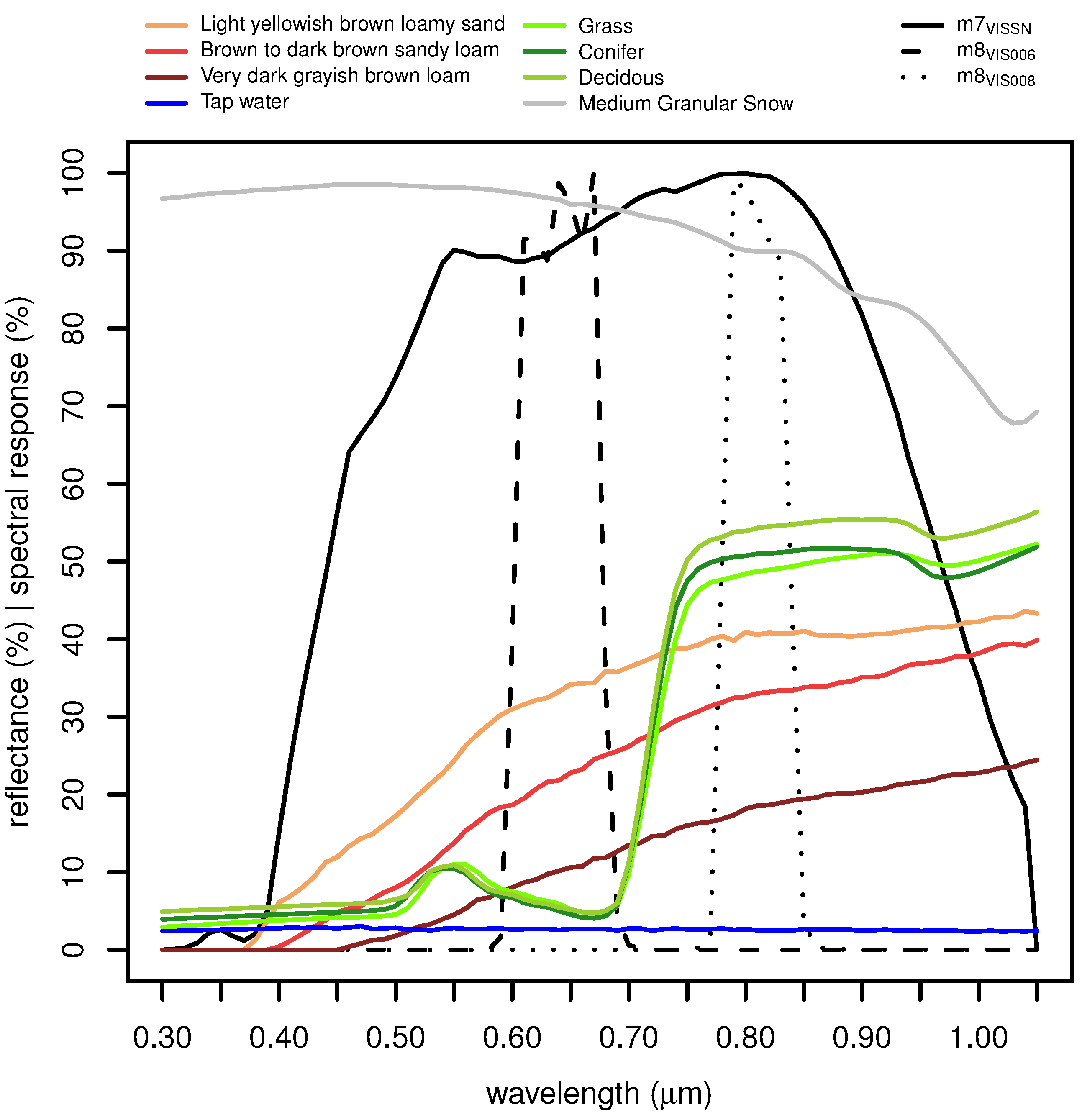
The spectral response functions of the MVIRI and the SEVIRI instruments on Meteosat 7 and 8, respectively, are presented in Figure 1 together with the spectral reflectances for various surface types obtained from the ASTER spectral library (http://speclib.jpl.nasa.gov) [5]. It can be seen that the surface reflectance of vegetated areas has a strong wavelength dependency on the reflection in this spectral region that might pose problems. This issue was already discovered within the HelioClim project by Cros et al. [6]. They proposed the generation of an artificial MVIRI VISSN channel from SEVIRI’s VIS006 and VIS008 by the linear combination of both channels [7]. However, they do no address or investigate homogeneity issues in their publication.

Figure 1. Spectral response functions for the Meteosat-7 (M7) and Metoesat-8 (M8) visible channels and the spectral reflectance for various surfaces.

Figure 1. Spectral response functions for the Meteosat-7 (M7) and Metoesat-8 (M8) visible channels and the spectral reflectance for various surfaces.

The present study investigates whether the climate Heliosat version with its self-calibration method is able to automatically account for the spectral and technological differences between MVIRI and SEVIRI. This would imply that the 23-year MVIRI SIS CDR ending in 2005 could be prolonged into the present with the help of the SEVIRI instruments on the MSG satellites without the need to artificially simulate a broadband channel. Furthermore, the results of this study will be useful in the attempt to extend the SIS CDR to other geostationary satellites (e.g., GOES) with differing spectral specifications.

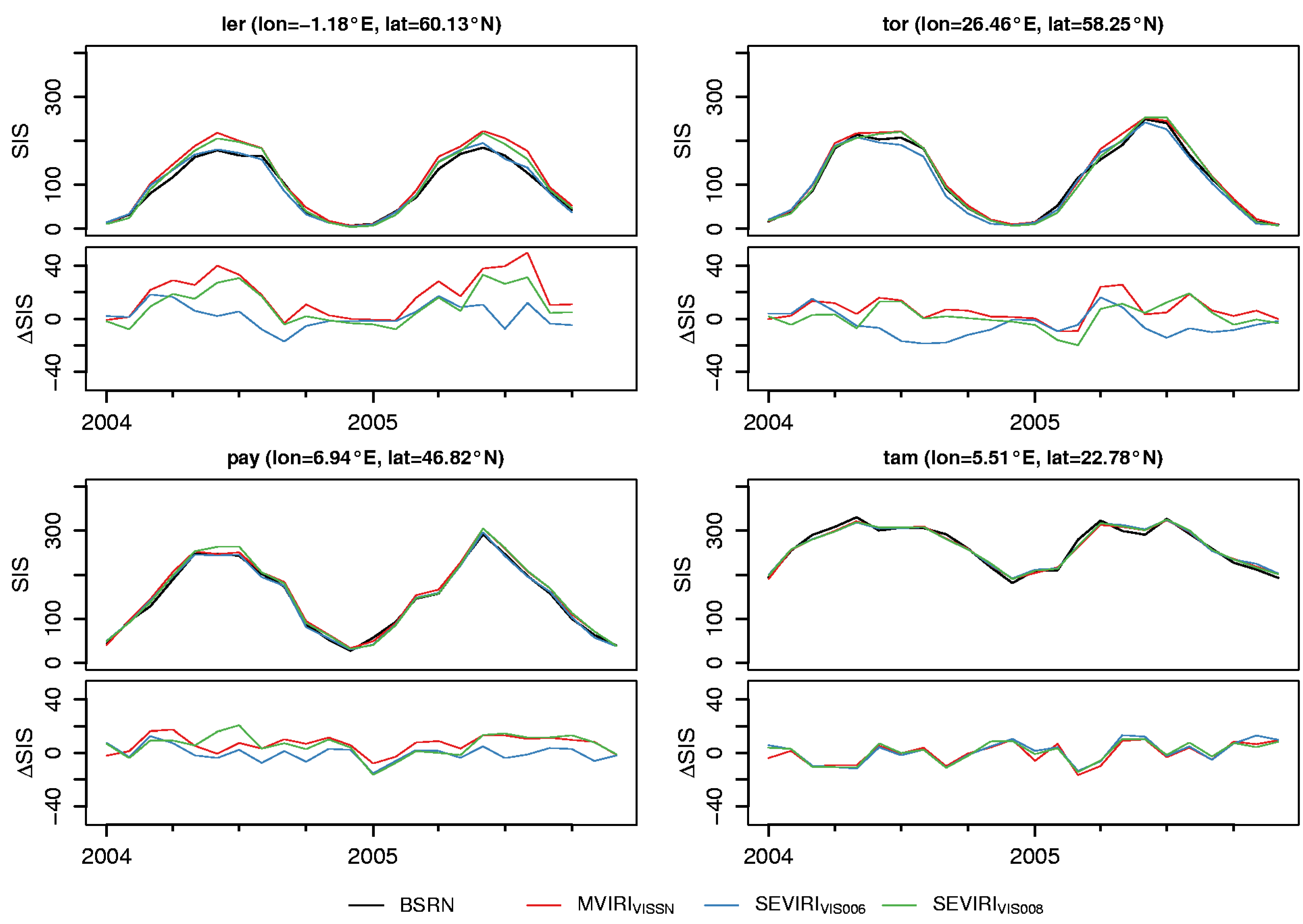
The following Section 2 describes the Heliosat algorithm used to derive the surface radiation from the satellite measurements including the applied modifications. Section 3 presents the results of the study by directly comparing the results of the different satellites and channels and by comparing them to surface measurements from the Baseline Surface Radiation Network (BSRN [8]). In Section 4 the results are presented, analyzed and discussed. The last Section 5 summarizes the results and concludes this study.

2. Methods and Data

2.1. Heliosat

The solar surface irradiance is derived from the geostationary satellite measurements in a two-step approach. First, the Heliosat algorithm uses the reflectance or radiance measurements to determine the effective cloud albedo n (also denoted as cloud index) [2,3,9]. In a second step, a clear sky model is used to calculate the solar surface (or global) irradiance (SIS) based on the retrieved effective cloud albedo.

Traditionally, the Heliosat algorithm uses the digital count D of the visible satellite channel. In this way, it neither depends on any calibration information nor on information from other channels. The effective cloud albedo is defined by the relation of the current satellite measurement and the corresponding observations under clear-sky conditions for the same satellite pixel. The brighter the pixel the more or thicker clouds are present.

The effective cloud albedo (n) is derived from the normalized counts ρ (i.e., accounting for the dark offset, the solar zenith angle and the sun-earth distance), the clear sky normalized counts ${\rho }_{cs}$ and the normalized counts of a compact (not convective) cloud deck as an estimation for the maximum possible normalized count ${\rho }_{max}$ by

$$n={\displaystyle \frac{\rho -{\rho }_{cs}}{{\rho }_{max}-{\rho }_{cs}}}$$

(1)

The clear sky normalized count is determined for every pixel separately as the minimum value of normalized counts ρ during a certain time period (e.g., one month). The “maximum” normalized count can be determined in a similar fashion by choosing the maximum ρ per pixel and time span [3] or by using a single value for the full disk that is dependent on the radiometer of the different satellites [9]. Here, the maximum normalized count is used in the new self-calibration method as presented in Section 2.2. Also, a revised method to determine the minimum normalized count is used in the present paper as outlined in Section 2.2.

The clear sky irradiance SIS${}_{cs}$ is calculated using an eigenvector look-up table method [10]. It is based on the libRadtran radiative transfer model ([11], http://www.libradtran.org) and enables the use of extended information about the atmospheric state. Accurate analysis of the interaction between the atmosphere, surface albedo, transmission and the top of atmosphere albedo has been the basis for the new method, characterized by a combination of parameterizations and “eigenvector” look-up tables. The source code of the method (Mesoscale Atmospheric Global Irradiance Code – MAGIC) is available under gnu-public license at: http://sourceforge.net/projects/gnu-magic/.

SIS is derived by the combination of effective cloud albedo n and clear sky irradiance SIS${}_{cs}$.

$$SIS=k\left(n\right)·SI{S}_{cs}$$

(2)

Thereby, $k\left(n\right)$ denotes the clear sky index which relates to n through the following relation [9]:

$$k\left(n\right)=\left\{\begin{array}{cc}1.2\hfill & \text{for}n\le 0.2\hfill \\ 1-n\hfill & \text{for}-0.2<n\le 0.8\hfill \\ 2.0667-3667n+1.6667n^2\hfill & \text{for}0.8<n\le 1.1\hfill \\ 0.05\hfill & \text{for}n>1.1\hfill \end{array}\right.$$

(3)

Consequently, for effective cloud albedo values between 0 and 0.8 SIS is given by equation

$$SIS=(1-n)·SI{S}_{cs}$$

(4)

In this range the solar surface irradiance is simply defined by the clear sky irradiance which is not reflected back to space by clouds. This relation can be derived by the law of energy conservation under the assumption of negligible absorption on cloud droplets.

2.2. Heliosat Modifications

Self-Calibration

The self-calibration method is based on the determination of the “maximum” normalized count ${\rho }_{max}$ that serves as the self-calibration parameter. The effect of different brightness sensitivities of the MVIRI instruments on SIS has been recognized and corrected with an ${\rho }_{max}$ approach by Hammer [12] in order to improve the accuracy and temporal homogeneity of satellite derived solar surface irradiance across the MVIRI instruments. Within the scope of the updated Heliosat method a histogram of all observed normalized counts is generated, in analogy to Rigollier et al. [13] . However, instead of using an upper and a lower bound as in Rigollier et al. [13], only the $95\%$-percentile is used as the self-calibration parameter and set to ${\rho }_{max}$. The use of the $95\%$ percentile for ${\rho }_{max}$ results in the largest stability of the self-calibration parameter. The use of a percentile value and not the maximum of the distribution excludes saturated pixels and convective clouds which would introduce too much month-to-month variability that would reduce the stability of the method.

The analysis of the full disk is computationally too expensive, hence, a regional subset of the full disk was selected. This region is located in the southern Atlantic between ${15}^{\circ }$W to $0^{\circ }$W and ${58}^{\circ }$S to ${48}^{\circ }$S. It features a frequent appearance of frontal systems with high cloud amounts but hardly any deep convective clouds. The self-calibration algorithm is applied to the 1300 UTC slot, which accounts for the slight westward shift of the region. The histograms are generated each month with all normalized counts at 1300 UTC of the respective month. The resulting ${\rho }_{max}$ is then applied to calculate the effective cloud albedo n for that month following Equation (1).

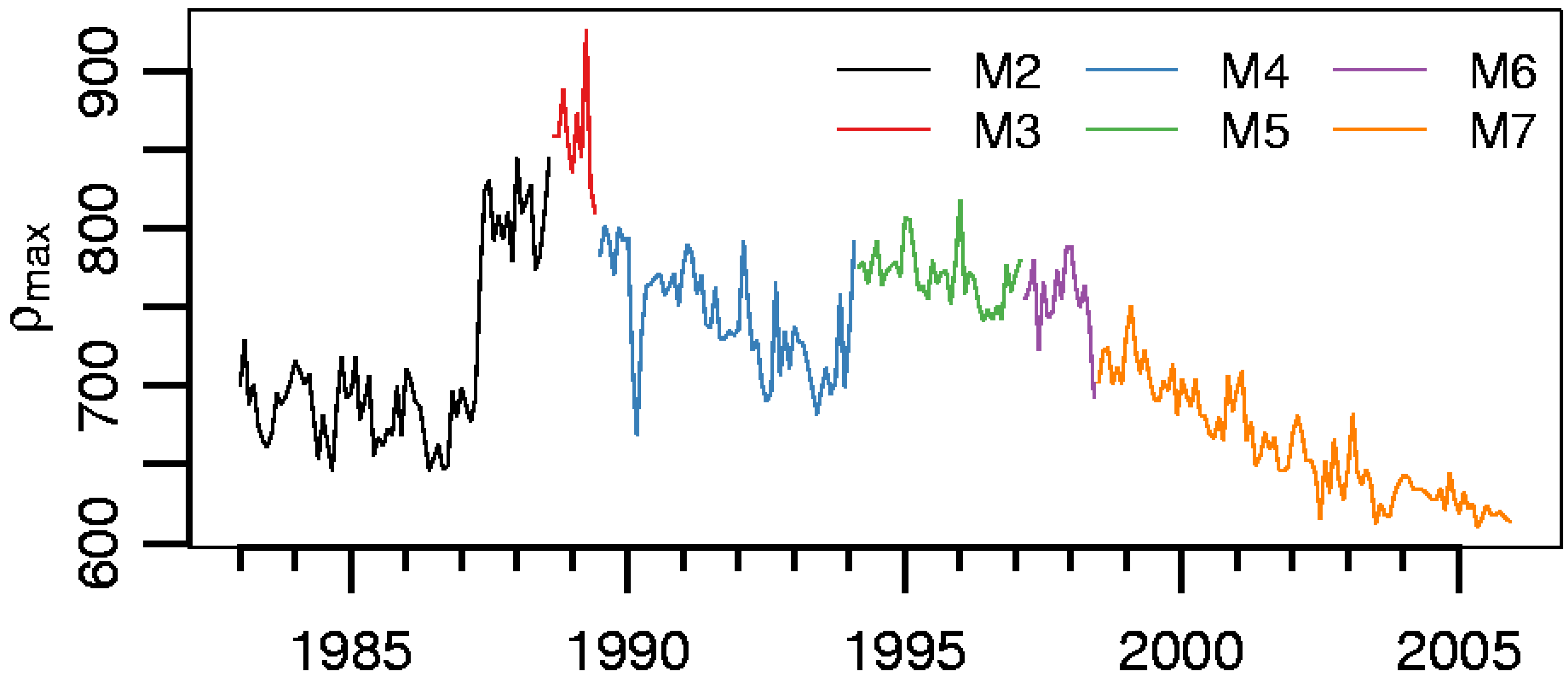
Figure 2 shows the temporal evolution of ${\rho }_{max}$ for the MVIRI period from 1983 to 2005 for the different MFG satellites. It can be seen that ${\rho }_{max}$ decreases substantially with the operation time of a satellite (e.g., Meteosat 7) which reflect the degradation of the instrument with time. Further gain changes in the instrument are also visible as seen for Meteosat 2. However, the differences of ${\rho }_{max}$ for the times of satellite replacements are comparably small. This shows that the self-calibration is able to capture the sensitivity changes (i.e., calibration) within the lifetime of the used instrument and, thus, ${\rho }_{max}$ can serve as parameter to calibrate the time series towards a homogeneity.

Figure 2. Temporal evolution of ${\rho }_{max}$ for the MVIRI period from 1983 to 2005. The Meteosat satellites (Meteosat 1–7) are illustrated in different colors.

Figure 2. Temporal evolution of ${\rho }_{max}$ for the MVIRI period from 1983 to 2005. The Meteosat satellites (Meteosat 1–7) are illustrated in different colors.

By definition the Heliosat method retrieves the effective cloud albedo. This circumvents the requirement to use land surface targets to calibrate the satellite radiances. In fact, by using a land surface target in the self-calibration method errors could be introduced as the aging detected by observation of clear sky radiances is different than that detected with an appropriate cloud target. This effect is due to spectral dependency of the aging of optical devices (“UV is more aggressive"), which leads to different rates of aging for different land surface types, due to different spectral response of the targets. In our self-calibration method the aging effects of the “clear sky” observations for different surface types is automatically considered by the retrieval of the clear sky normalized digital counts ${\rho }_{cs}$.

Govaerts et al. [14] developed a calibration method at EUMETSAT in support of meteorological and climate applications. The method relies on radiative transfer modeling over bright deserts as the primary calibration target type. Open sea surface targets are used to verify the consistency and reliability of the results. Results obtained for the calibration of Meteosat-5 and -7 demonstrate that it is possible to calibrate the VIS band with an estimated accuracy of about $\pm 6\%$, but this error increases as the uncertainty of the sensor spectral response characterization increases [14]. However, this method is not an appropriate alternative due to the relative low calibration accuracy and the use of a desert target.

Clear Sky Retrieval

A recently developed clear sky algorithm for Heliosat is used to calculate ${\rho }_{cs}$ [15]. In the original Heliosat method the clear sky value ${\rho }_{cs}$ has been derived by estimation of the minimum ρ value within a month for each slot. Instead of using monthly fields of the normalized counts ρ, a seven day running value of ${\rho }_{cs}$ is used in the Heliosat version discussed herein. Thus, ${\rho }_{cs}$ is allowed to change within a month. Thus, changes in ${\rho }_{cs}$, e.g., due to changes in the vegetation and snow cover, are captured and represented faster than with the standard method. In addition, unrealistic steps in ${\rho }_{cs}$ between different months are avoided. Further on, the presented clear sky algorithm allows the detection of snow and, thus, provides the opportunity to correct for some of the radiative properties of snow.

The reduction of the period applied for the retrieval of the clear sky reflection background leads to a reduction of the probability for the occurrence of cloud-free cases. Hence a simple minimum method can no longer be applied in order to avoid systematic cloud contamination. Tests on the temporal evolution of ${\rho }_{cs}$ have to be applied to avoid systematic cloud contamination of ${\rho }_{cs}$ and to detect changes in ${\rho }_{cs}$ due to snow. The tests are aimed to enable the distinction between a real increase in ${\rho }_{cs}$ given by snow and an artificial increase induced by clouds. The algorithm to determine ${\rho }_{cs}$ is based on two tests that are applied to the normalized counts (ρ) in order to determine the temporal evolution of ${\rho }_{cs}$. If both tests fail, i.e., if ρ is rather large as occurring in case of clouds and snow, ${\rho }_{cs}$ is not changed. In the following, the subscript t denotes the current and $t+1$ the subsequent time step.

$$\text{Test}\text{1}:{\rho }_{cs,t}\le {\rho }_t\le {\rho }_{cs,t}+{ϵ}_{up}\text{or}{\rho }_t<{\rho }_{cs,t}-{ϵ}_{low}$$

$$\to {\rho }_{cs,t+1}={\displaystyle \frac{6}{7}}{\rho }_{cs,t}+{\displaystyle \frac{1}{7}}{\rho }_t(\text{slow}\text{evolution})$$

(5)

$$\text{Test}\text{2}:{\rho }_{cs,t}-{ϵ}_{low}\le {\rho }_t<{\rho }_{cs,t}$$

$$\to {\rho }_{cs,t+1}={\displaystyle \frac{1}{2}}{\rho }_{c{s}_t}+{\displaystyle \frac{1}{2}}{\rho }_t(\text{fast}\text{evolution})$$

(6)

$$\begin{array}{cc}\hfill \text{else}:& {\rho }_{cs,t+1}={\rho }_{cs,t}\hfill \end{array}$$

(7)

Here we use variable bandwidths ${ϵ}_{up}$ and ${ϵ}_{low}$ depending on ${\rho }_{max}$ and ${\rho }_{cs}$ ([15] and personal communication).

$$\begin{array}{cc}\hfill {ϵ}_{up}& =0.125{\rho }_{max}+{\displaystyle \frac{8({\rho }_{cs}-0.15{\rho }_{max})}{0.25{\rho }_{max}}}\hfill \end{array}$$

(8)

$$\begin{array}{cc}\hfill {ϵ}_{low}& =0.0875{\rho }_{max}+{\displaystyle \frac{6({\rho }_{cs}-0.15{\rho }_{max})}{0.25{\rho }_{max}}}\hfill \end{array}$$

(9)

If both tests fail for $t_s=28$ subsequent days (i.e., the pixel is very bright at all times) then this pixel is assigned to be snow covered. This time-series approach by Zelenka [16] is based on the low temporal variability of snow compared to clouds. Thus, continuously detecting very high reflectivities in one time slot over a certain number of days indicate snow. This strategy can fail in the cases of persistent cloud decks (e.g., marine stratocumulus or fog). In case of a positive snow detection (i.e., $t_s$ is reached) ${\rho }_{cs}$ subsequently evolves according to Equation (6) so that ${\rho }_{cs}$ increases to the range of the current minimum normalized counts and the basic scheme (i.e., Test 1 and Test 2) can be applied in the subsequent time steps.

In order to better account for snowfall events, $t_s$ is reduced to seven in case the considered pixel already had a snow event. This is given by either an amplitude $\Delta {\rho }_{cs}={\rho }_{cs,max}-{\rho }_{cs,min}$ exceeding $0.55{\rho }_{max}$ or by ρ being larger than a snow threshold ${\rho }_{snow}$. Latter is derived empirically so that it is high enough to exclude oceans or other dark surfaces (${\rho }_{snow,min}$) and that it favors pixels that have a high $\Delta {\rho }_{cs}$ and thus a higher probability of a former snow event (${\rho }_{snow,range}$).

$$\begin{array}{cc}\hfill {\rho }_{snow,min}& =0.48{\rho }_{max}\hfill \end{array}$$

(10)

$$\begin{array}{cc}\hfill {\rho }_{snow,range}& =max(0.15{\rho }_{max},0.6\Delta {\rho }_{cs})\hfill \end{array}$$

(11)

$$\begin{array}{cc}\hfill {\rho }_{snow}& =max({\rho }_{snow,min},{\rho }_{cs,min}+{\rho }_{snow,range})\hfill \end{array}$$

(12)

The calculation of the effective cloud albedo n for non-snow pixels follows the standard Heliosat method (see Equation (1)). In case snow is detected the calculation of the cloud albedo n is altered according to [15] in which ${\rho }_{cs}$ is substituted by ${\rho }_{snow,min}$ and ${\rho }_{max}$ is increased by a factor of $1.41$ in order to artificially increase the count range and, thus, enhance the contrast. This altered cloud albedo formulation generally gives lower cloud albedo values in order to account for the radiative properties of snow. This includes mainly the reflectivity of the bright snow surface which leads to higher surface irradiance values.

$$n_s={\displaystyle \frac{\rho -0.48{\rho }_{max}}{1.41{\rho }_{max}-0.48{\rho }_{max}}}={\displaystyle \frac{\rho -0.48{\rho }_{max}}{0.93{\rho }_{max}}}$$

(13)

2.3. Satellite Data

Data from EUMETSAT’s geostationary Meteosat satellites of the First and Second Generation are used in the present study. The satellites were located over the equator at a longitude of $0^{\circ }$ at an altitude of about 36,000 km. The field of view of both satellites reaches up to 80${}^{\circ }$N/S and 80${}^{\circ }$E/W, respectively.

The MFG satellites (Meteosat 2–7, in operation 1982–2005) carried the Meteosat Visible and InfraRed Imager (MVIRI), a radiometer with 3 spectral bands in the visible band (VISSN: 0.45–1 $\mu \text{m}$), in the water vapor band (WV: 5.7–7.1 $\mu \text{m}$) and infrared band (IR: 5.7–7.1 $\mu \text{m}$). One scan of the visible disc was accomplished within 30 min at a horizontal resolution of around 2.5 km at the sub-satellite point.

The MSG satellites (Meteosat 8–9, in operation since 2004) carry the Spinning Enhanced Visible and InfraRed Imager (SEVIRI), a radiometer that measures in 12 different spectral bands in the visible and infrared spectral region at a horizontal resolution of around 3 km every 15 min. The two visible channels measure at narrow bands around 0.6 $\mu \text{m}$ (VIS006) and 0.8 $\mu \text{m}$ (VIS008). Additionally, there is a broadband high resolution visible (HRV) channel with a spatial resolution of around 1 km. However, due to a satellite failure this channel does not work properly, e.g., does not cover the full disk.

This study encompasses the overlap time period between the two satellite generations in the years 2004 and 2005, when Meteosat 7 and 8 were measuring side by side. Meteosat 8 was, however, slightly shifted eastward to 3.4${}^{\circ }$E.

The input data from the MVIRI and the SEVIRI instruments were obtained from Eumetsat’s UMARF archive in the OpenMTP or Native format, respectively. The output data (global and direct radiation and cloud albedo) were re-gridded to a regular lon-lat grid with a 0.03${}^{\circ }$ grid spacing using a triangulation technique (provided within the programming language IDL).

2.4. Ground Based Measurements

The quality of the satellite-derived SIS is evaluated with the help of ground based station data from the Baseline Surface Radiation Network (BSRN, [8]).

BSRN is a project of the World Climate Research Program (WCRP) and the Global Energy and Water Experiment (GEWEX). The aim of the BSRN is to provide consistent quality-controlled surface radiation data from a global station network using a defined set of instrumentation and measurement protocols. Currently, about 50 surface stations are operating in different climatic zones. The data are collected and stored at the Alfred-Wegener Institute for Polar Research (AWI) and made publicly available at http://www.bsrn.awi.de (FTP and web access). The accuracy of the short-wave measurement is estimated to be 5 $W{m}^{-2}$ [8]. Here, we use the surface data obtained at the 10 stations that are within the full disc of the Meteosat satellite for the years 2004 and 2005 (see Table 1) as a reference to evaluate the quality of the satellite-derived data sets.

Table 1. Relevant BSRN stations present on the Meteosat full disk for the years 2004 to 2005.

	Place/Region	Latitude	Longitude	Height
		${[}^{\circ }]\text{N}$	${[}^{\circ }]\text{E}$	$[\mathrm{m}\mathrm{a}.\mathrm{s}.\mathrm{l}.]$
ber	Bermuda (BM)	32.27	–64.67	8
cam	Cambourne (GB)	50.22	–5.32	88
car	Carpentras (FR)	44.08	5.06	100
daa	DeAar (ZA)	–30.67	23.99	1,287
ler	Lerwick (GB)	60.13	–1.18	84
pal	Palaiseau (FR)	48.71	2.21	156
pay	Payerne (CH)	46.82	6.94	491
sbo	Sede Boqer (IL)	30.91	34.78	500
tam	Tamanrasset (DZ)	22.78	5.51	1,385
tor	Toravere (EST)	58.25	26.46	70

Table 1. Relevant BSRN stations present on the Meteosat full disk for the years 2004 to 2005.

	Place/Region	Latitude	Longitude	Height
		${[}^{\circ }]\text{N}$	${[}^{\circ }]\text{E}$	$[\mathrm{m}\mathrm{a}.\mathrm{s}.\mathrm{l}.]$
ber	Bermuda (BM)	32.27	–64.67	8
cam	Cambourne (GB)	50.22	–5.32	88
car	Carpentras (FR)	44.08	5.06	100
daa	DeAar (ZA)	–30.67	23.99	1,287
ler	Lerwick (GB)	60.13	–1.18	84
pal	Palaiseau (FR)	48.71	2.21	156
pay	Payerne (CH)	46.82	6.94	491
sbo	Sede Boqer (IL)	30.91	34.78	500
tam	Tamanrasset (DZ)	22.78	5.51	1,385
tor	Toravere (EST)	58.25	26.46	70

3. Results

3.1. Comparison with Ground Based Measurements

The ground based measurements of BSRN are used for the validation of the SIS retrieval from MVIRI and SEVIRI (see Section 2.4).

As shown in Figure 3, the mean absolute bias (MAB) for these cases is mostly below the threshold of 15 ${\mathrm{Wm}}^{-2}$. This threshold value is composed of the 10 ${\mathrm{Wm}}^{-2}$ accuracy requirement for solar surface irradiance retrieved from satellites as defined by the Global Climate Observing System (GCOS) and a measurement uncertainty of the short-wave BSRN surface data of 5 ${\mathrm{Wm}}^{-2}$ [8].

Figure 3. Bias and MAB for the comparison of satellite retrieved SIS versus BSRN measurements of all relevant BSRN stations and for first and second generation satellites.

Figure 3. Bias and MAB for the comparison of satellite retrieved SIS versus BSRN measurements of all relevant BSRN stations and for first and second generation satellites.

The monthly mean SIS time series from the surface measurements and the three satellite-based retrieval results are shown in Figure 4 for four selected stations (tor, ler, pay, tam). In general, the surface measurement and the satellite retrievals as well as the different satellite retrievals compare well.

Figure 4. Comparison of satellite retrieved SIS versus BSRN measurements for 4 selected stations.

Figure 4. Comparison of satellite retrieved SIS versus BSRN measurements for 4 selected stations.

Larger differences between the surface measurements and the satellite-derived SIS occur at the station of Lerwick (ler), especially for the MVIRI-derived surface radiation (see Figure 3 and Figure 4). Because the location of Lerwick is close to the northern rim of the Meteosat full disc and in a region with high spacial and temporal cloud cover, the accuracy of the satellite-derived SIS, especially from the MVIRI instrument, is reduced. Another station far up north is Toravere (tor, Estonia). The spread of the absolute differences (marked by the box and the whiskers) is also relatively large but not as large as for Lerwick. The more continental position results in lesser cloud amount and more clear-sky cases than at Lerwick which gives comparably better estimates for ${\rho }_{cs}$ and SIS. However, the determination of ${\rho }_{cs}$ is still more problematic than at other stations. The station of Bermuda (ber) which is located close to the (western) rim of the Meteosat full disc but in a much less cloudy region with much more clear-sky days does not show large deviations from the BSRN data. These findings point to problems in the determination of the clear-sky normalized counts ${\rho }_{cs}$ in very cloudy regions close to the rim of the disc. This will be further discussed in Section 4 below.

The differences between the satellite-derived SIS (purple and orange bars in Figure 3) are smaller or at least comparable to the differences between the satellite-derived and the surface measured SIS data. This indicates that for the considered stations the satellite retrieved surface radiation can be regarded as equivalent. As already shown in Table 2 and, additionally, in Figure 3, the retrieval based on the SEVIRI VIS008 channel compares slightly better with the MVIRI retrieval than the retrieval based on the SEVIRI VIS006 channel.

Hence, the SEVIRI VIS008 channel seems to be better suited to extend the MVIRI SIS time series than the VIS006 channel. However, the overall quality of the satellite-retrieved SIS data set is higher when the SEVIRI VIS006 channel is used. Further studies are required to extend the MVIRI SIS data set to the SEVIRI time series.

3.2. Self-calibration

The self-calibration method (see Section 2.2) works properly for the retrieval of the surface solar irradiance for the series of MVIRI satellite instruments as depicted in Figure 5 which shows the trend in the normalized bias between the BSRN stations and the derived solar surface irradiance SIS in the time range from 1994 to 2005.

Figure 5. Temporal evolution of the normalized bias between the CM SAF data set and the BSRN data. Changes in the satellite instruments are indicated by the blue lines on the x-axis. The green line represents the zero line, the red line is the linear regression.

Figure 5. Temporal evolution of the normalized bias between the CM SAF data set and the BSRN data. Changes in the satellite instruments are indicated by the blue lines on the x-axis. The green line represents the zero line, the red line is the linear regression.

The normalized bias is calculated as follows: The arithmetic average over the complete time series of the BSRN and the satellite data is calculated. The resulting bias is then subtracted from all monthly means of the satellite data time series. This two steps are performed for every station. The bias for each station site is zero afterwards, however, trends in the monthly bias values are not affected by this normalization procedure. The differences (normalized bias values) between the monthly means of BSRN and satellite data are then averaged over all available stations for each month, whenever monthly means from at least 3 stations are available. This leads to an overall time series of “normalized bias” values of the monthly means. This time series is then analyzed for temporal trends.

The fitted linear line (red line, 0.062 $W{m}^{-2}y{r}^{-1}$) is statistically not significant, hence no temporal trend is apparent. A trend in this time series would indicate in-homogeneities introduced by the self-calibration or the clear sky reflection method. Also the changes between the different satellite sensors (marked with the blue lines) are not visible.

The normalization procedure has to be applied in order to avoid misleading trends in the monthly bias values introduced by the quite different start and end points of the time series and the corresponding mismatch in the weighting of regional bias values.

Here we evaluate whether the Heliosat climate version with its self-calibration method is able to account for the spectral and technological differences introduced by the transition from the MVIRI broadband VIS to the SEVIRI VIS006 or VIS008 channels in the Heliosat algorithm. During the transition period 2004 and 2005 data from both satellite instruments are available, which allows the investigation of the impact of the change in the satellite instruments on the stability and the homogeneity of the retrieved SIS CDR.

The upper panel of Figure 6 shows the temporal evolution of ${\rho }_{max}$ for the different satellite instruments and channels. The annual variability is in all cases within a range of 20–30 normalized counts. A slight decay of ${\rho }_{max}$ over time is also visible which corresponds to the degradation of the satellite instruments over time which is compensated by the Heliosat method. The normalized counts from MVIRI and from the VIS008 channel of SEVIRI are quite similar while the ${\rho }_{max}$ of SEVIRI’s VIS006 channel is about 30–50 counts higher.

The lower panel of Figure 6 shows the lower end of the range of normalized counts. ${\rho }_{cs}$ is the “minimum” of of the count distribution (clear sky reflection) within the selected area (see Section 2.2). The difference between ${\rho }_{max}$ and ${\rho }_{cs}$ provides a good estimate of the range of the normalized counts that can be used to determine the cloud albedo. As can be seen, ${\rho }_{cs}$ is quite similar for MVIRI and for the VIS006 channel of SEVIRI. However, for the VIS008 channel of SEVIRI the ocean surface appears about 30–50 counts darker than for the former two. Overall, it can be summarized that the range of the two SEVIRI channels is about 30–50 counts larger over ocean than the MVIRI range. Over land surfaces, however, this difference is lower because of the higher values for the minimum count value. The implications of the different ranges for the two instruments on the derived solar surface irradiance are explained in Section 4.

The absolute differences of the seasonal means for Winter (DJF, upper row) and Summer (JJA, lower row) between solar surface irradiance derived from MVIRI and from the two SEVIRI channels (left column for VIS006, right column for VIS008) are shown in Figure 7. Blue colors denote higher global radiation values for MVIRI than for SEVIRI and vice versa for red colors.

Figure 6. ${\rho }_{max}$ and ${\rho }_{cs}$ (${\rho }_{max}$) for MVIRI and SEVIRI visible channels.

Figure 6. ${\rho }_{max}$ and ${\rho }_{cs}$ (${\rho }_{max}$) for MVIRI and SEVIRI visible channels.

Figure 7. Seasonal differences (DJF: top row, JJA: bottom row.) between Meteosat-7 (MVIRI) and Meteosat-8 (SEVIRI) visible channels (VIS006: left column, VIS008: right column).

Figure 7. Seasonal differences (DJF: top row, JJA: bottom row.) between Meteosat-7 (MVIRI) and Meteosat-8 (SEVIRI) visible channels (VIS006: left column, VIS008: right column).

Table 2 quantifies the differences between the solar surface irradiance derived from MVIRI broadband channel and the SEVIRI channels VIS006 and VIS008 as bias and mean absolute bias (MAB). The MAB between the solar surface irradiance derived from the two instruments is below 4 ${\mathrm{Wm}}^{-2}$ for both SEVIRI channels. On average, both SEVIRI channels yield a lower solar surface irradiance than the broadband VIS channel of the MVIRI instrument. While the use of the VIS006 SEVIRI channel always results in lower surface irradiance, application of the VIS008 channel can result in higher surface irradiance than the use of the MVIRI channel, especially over vegetated areas (see Figure 7).

Table 2. Bias and MAB between Meteosat 7 and the different channels of Meteosat 8.

		${\mathrm{SEVIRI}}_{\mathrm{VIS}006}$	${\mathrm{SEVIRI}}_{\mathrm{VIS}008}$
		$-{\mathrm{MVIRI}}_{\mathrm{VISSN}}$
Bias	$\left[{\mathrm{Wm}}^{-2}\right]$	–3.39	–2.10
MAB	$\left[{\mathrm{Wm}}^{-2}\right]$	3.88	3.59

Table 2. Bias and MAB between Meteosat 7 and the different channels of Meteosat 8.

		${\mathrm{SEVIRI}}_{\mathrm{VIS}006}$	${\mathrm{SEVIRI}}_{\mathrm{VIS}008}$
		$-{\mathrm{MVIRI}}_{\mathrm{VISSN}}$
Bias	$\left[{\mathrm{Wm}}^{-2}\right]$	–3.39	–2.10
MAB	$\left[{\mathrm{Wm}}^{-2}\right]$	3.88	3.59

While the mean difference between the solar surface irradiance derived from MVIRI and SEVIRI is rather low, local differences can be higher. This is especially visible for vegetated areas (South America, Tropical Africa and Europe in Summer). The following Section 4 discusses the potential effects that might result in the observed differences.

4. Discussion

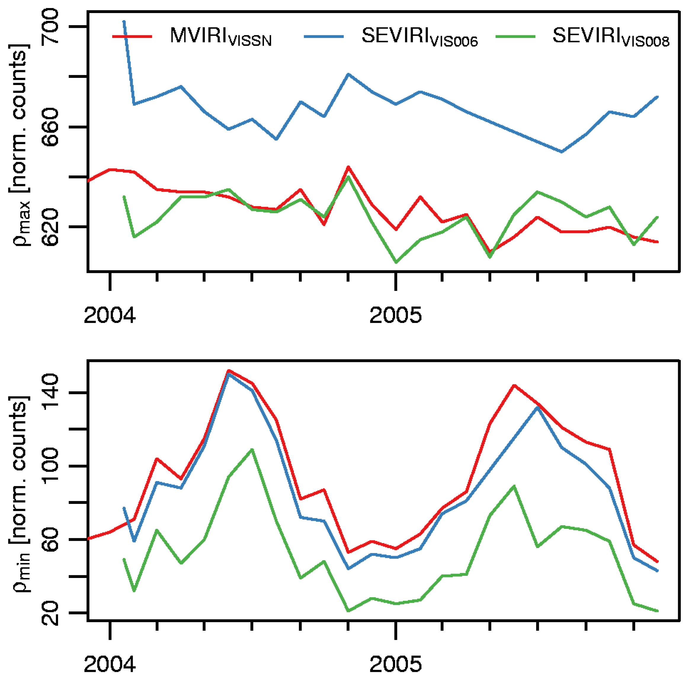
Section 3 on the results showed that the differences between the SIS retrievals from MVIRI and SEVIRI can be locally quite large. Two major effects are found that help to understand those differences. The first major effect originate from the different spectral properties of the MVIRI and SEVIRI visible channels (see Figure 1) whereas the second effect bases on the different normalized count range available for the determination of n (see Figure 6).

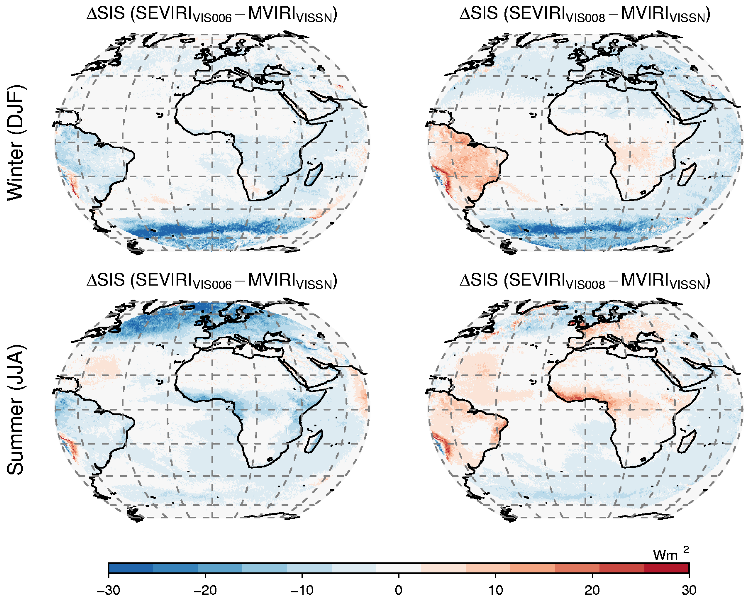
(a) Spectral effect: The impact of the different wavelengths and bandwidths of the satellite channels is apparent especially over vegetated areas (i.e., South America, tropical Africa and Europe in summer). This effect is particularly strong for the VIS008 channel because the high reflectance of vegetation at this wavelength results in an increase of the clear sky normalized counts compared to the MVIRI clear sky normalized counts. This reduced contrast between ρ and ${\rho }_{cs}$ over vegetated areas is not fully compensated by the reduced difference between ${\rho }_{max}$ and ${\rho }_{cs}$, which leads to a reduction of the retrieved effective cloud albedo (especially for thin clouds with low values of ρ) and subsequently to an increase in the solar surface irradiance.

The opposite effect is found for the VIS006 channel where the very low reflectance of the vegetation increases the sensitivity of the method towards the detection of clouds and enhances the retrieved effective cloud albedo. However, the lower values of the retrieved solar surface irradiance using the VIS006 channel compared to the MVIRI channel are masked by the value range effect discussed next.

(b) Value range effect: As discussed previously, the SIS derived from SEVIRI data is on average slightly lower than that derived from MVIRI, indicating that the effective cloud albedo derived form SEVIRI is slightly higher than that derived from MVIRI measurements. This difference is particularly pronounced over dark surfaces (like the ocean) in combination with high cloudiness and slant viewing geometry.

The cause of this difference could be the larger range of SEVIRI normalized counts (see Section 3.2) that allows easier detection of clear sky relative to clouds as the contrast between ${\rho }_{cs}$ and ρ is larger. The clear sky normalized counts derived from SEVIRI most likely contain less contamination of thin clouds as their counts might be outside the test interval used in the algorithm to derive the clear sky normalized counts ${\rho }_{cs}-{ϵ}_{low}$ and ${\rho }_{cs}+{ϵ}_{up}$ (see Equations (5)–(7)) whereas in case of the MVIRI they might fall within this interval. Hence, ${\rho }_{cs}$ derived from MVIRI could be higher in comparison to ρ which then results in a smaller difference $\rho -{\rho }_{cs}$ and, thus, a lower n and higher SIS. Furthermore, the aging of the MVIRI instrument on Meteosat 7 might result in an even further decrease of the contrast as ${\rho }_{max}$ is decreasing with time. The ϵ bandwidth and limits applied within the snow detection method might be not longer appropriate for the aged contrast. Note, that Meteosat 7 has been operating already 7 years in 2004. Furthermore, Dürr and Zelenka [15] derived the ϵ for the SEVIRI instrument with the larger normalized counts range as basis. Hence, an adaption of the ϵ bandwidth to the lower count range of MVIRI might reduce the value range effect.

This effect of the larger normalized count range (i.e., lower ${\rho }_{cs}$) in the SEVIRI measurements is particularly pronounced in regions with slant viewing geometries combined with high spatial and temporal cloud cover (i.e., at the northern and southern rim of the visible disc which are within the respective mid-latitude storm tracks). Additionally, the vertical extend of the clouds combined with slant viewing geometries obstructs the view of the satellite to the surface. Thus, the satellite experience clear sky very seldom which results in the increase in ${\rho }_{cs}$ as the algorithm assumes the cloudy pixel to be clear and uses it for the determination of ${\rho }_{cs}$.

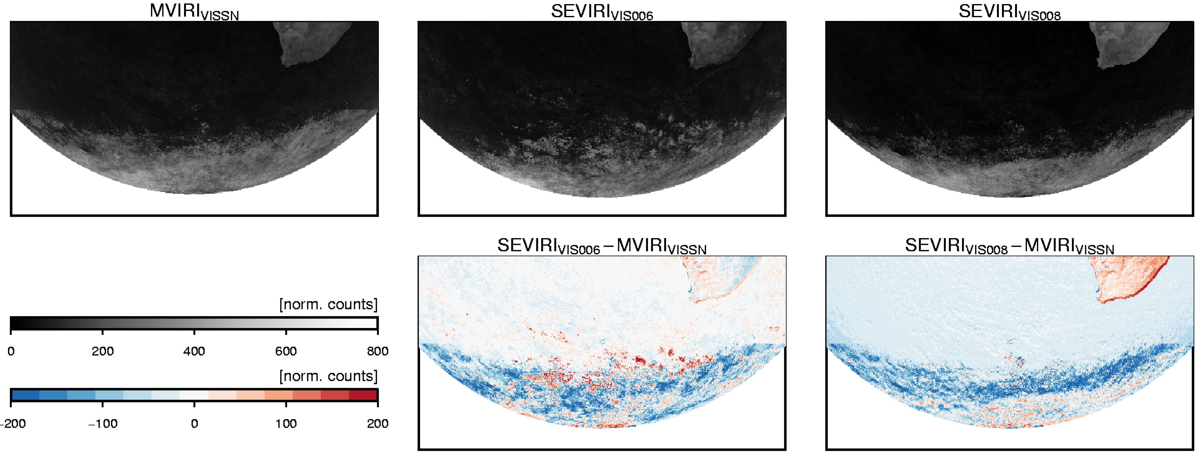
Figure 8 shows the clear sky normalized counts ${\rho }_{cs}$ for the southern rim of the Meteosat disc for the MVIRI and SEVIRI visible channels for January 2005. It can be seen that the cloud contamination of the ${\rho }_{cs}$ field is apparent for all satellite instruments and channels. However, for MVIRI the spatial extend is larger and, as the difference plots in Figure 3 suggests, also the magnitude.

The higher clear sky normalized counts also enhance the probability of increased snow detection in this regions. The threshold ${\rho }_{snow}$, which is close to ${\rho }_{snow,min}$ in this case, is exceeded very frequently due to the high values of ${\rho }_{cs}$ (${\rho }_{snow,range}$ is small, as ${\rho }_{cs}$ is relatively constant at a high level and, thus, $\Delta {\rho }_{cs}$ is small, see Equation (10)). Thus, the number of subsequent days $t_s$ with high clear sky normalized counts required to positively detect snow, has the lower value of six more often and in a larger regional extend for MVIRI than for SEVIRI. This results in a higher snow cover extent and consequently in the application of $n_s$ (see Equation (13)) which results in lower effective cloud albedo and higher solar surface irradiance values for MVIRI in these regions.

This effect of the enhanced snow detection under high viewing angles when using MVIRI measurements is a consequence of the short-comings in the snow detection testing of the clear sky radiance ${\rho }_{cs}$. Future versions of the snow detection algorithm should account for the special characteristics of the clear sky field close to the rim of the full disc. For the current data this implies that the data based on the MVIRI measurements at high slant viewing geometries (i.e., above a viewing angle of ${60}^{\circ }$) should be handled with care.

Figure 8. Clear sky normalized counts ${\rho }_{cs}$ for the southern rim of the Meteosat disc for the MVIRI and SEVIRI visible channels for January 2005 (12 UTC slot).

Figure 8. Clear sky normalized counts ${\rho }_{cs}$ for the southern rim of the Meteosat disc for the MVIRI and SEVIRI visible channels for January 2005 (12 UTC slot).

(c) Additional effect: While the above mentioned differences between the MVIRI and the SEVIRI are mainly responsible for the different retrieval results for SIS (as presented above) another factor might also contribute to the differences. The slightly different spatial resolutions of the instruments might introduce differences in the retrieved surface radiation especially in regions with broken cloud cover or heterogeneous land cover.

5. Summary and Conclusions

This study evaluated the ability of the climate version of Heliosat to automatically account for the spectral and technological differences between the MVIRI broadband visible channel onboard the MFG satellites and the SEVIRI narrowband VIS006 or VIS008 channels onboard the MSG satellites in the retrieval of the solar surface irradiance from satellites. This would enable the prolongation of the MFG-based SIS CDR to the present by using the MSG satellites. However, the results of this study demonstrate that the current Heliosat climate version is not able to compensate all effects arising by the transition from the MVIRI broadband visible to the SEVIRI narrowband VIS008 or VIS006 channels.

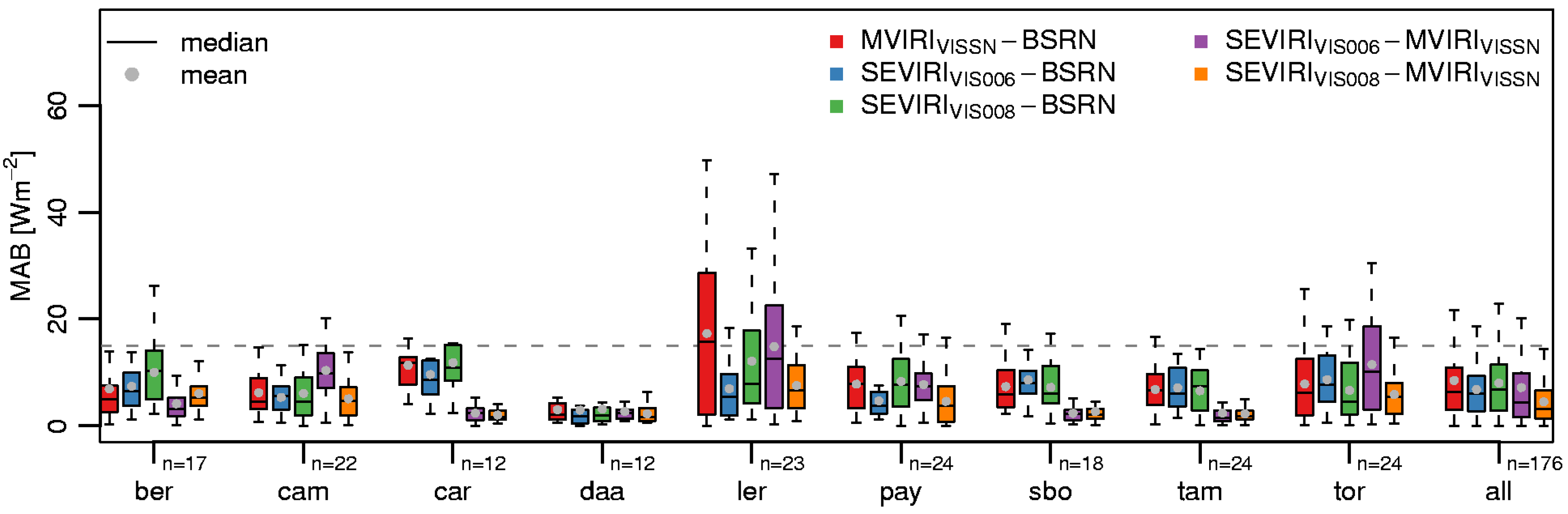
The comparison with BSRN station data demonstrates that the differences between both satellite generations (and channels) are in the same order or lower than the differences of the satellites to the stations. This could lead to the conclusion that the extension of the MFG-derived SIS CDR with MSG data might be possible. However, regions of large differences between the two satellite generations, such as the heavily vegetated interior of South America, have no BSRN station coverage.

The spectral differences between the channels of both sensors have a significant influence on the resulting SIS. This especially becomes evident for the highly vegetated areas of South America, tropical Africa and Europe (the latter only during summer) as the differences in the reflectances are most pronounced. The lower (higher) reflectance of vegetation of SEVIRI’s VIS006 (VIS008) channel compared to MVIRI results in a higher (lower) effective cloud albedo and a lower (higher) solar surface irradiance. The applied self-calibration method alone is not able to compensate the spectral differences of the channels.

Furthermore, the differences in the ranges of the normalized counts between the two satellite generations lead on average to lower SIS from SEVIRI, in line with surface observations. This can be explained by less cloud contamination in the surface albedo field due to a larger contrast between the surface and clouds. Therefore, the SEVIRI effective cloud albedo is on average more accurate, with higher values, which leads in turn to lower solar surface irradiance. This effect is particularly pronounced in regions with dark surfaces in combination with slant viewing geometry and large frequency of cloud occurrence. This enhances the probability of snow detection which additionally lowers the effective cloud albedo and increases solar surface irradiance.

In general, both satellite generations allow the generation of a SIS CDR that satisfies climate monitoring requirements of GCOS. We would therefore motivate the generation of a cross MFG-MSG SIS CDR that is for instance useful for climate monitoring and analysis of inter-annual variability and extremes. Trend analysis across the satellite generations should however be done carefully and might require temporal and spatial homogenization beforehand. The differences discussed in this paper are likely to be reduced by the use of an simulated visible broadband channel as discussed in [7].

The study has for the first time analyzed the effects of the MFG to MSG transition on the widely used Heliosat method. The above findings should be starting point for future research that aims to reduce the sensitivity of the Heliosat effective cloud albedo and its related properties on the spectral and technological differences of heritage, current and future satellite sensor generations. Additional work is especially needed when Heliosat is used with other geostationary satellites (such as GOES, GMS or FY) to build a global SIS climate data record.