A Hierarchical Spatio-Temporal Markov Model for Improved Flood Mapping Using Multi-Temporal X-Band SAR Data

Abstract
:
1. Introduction
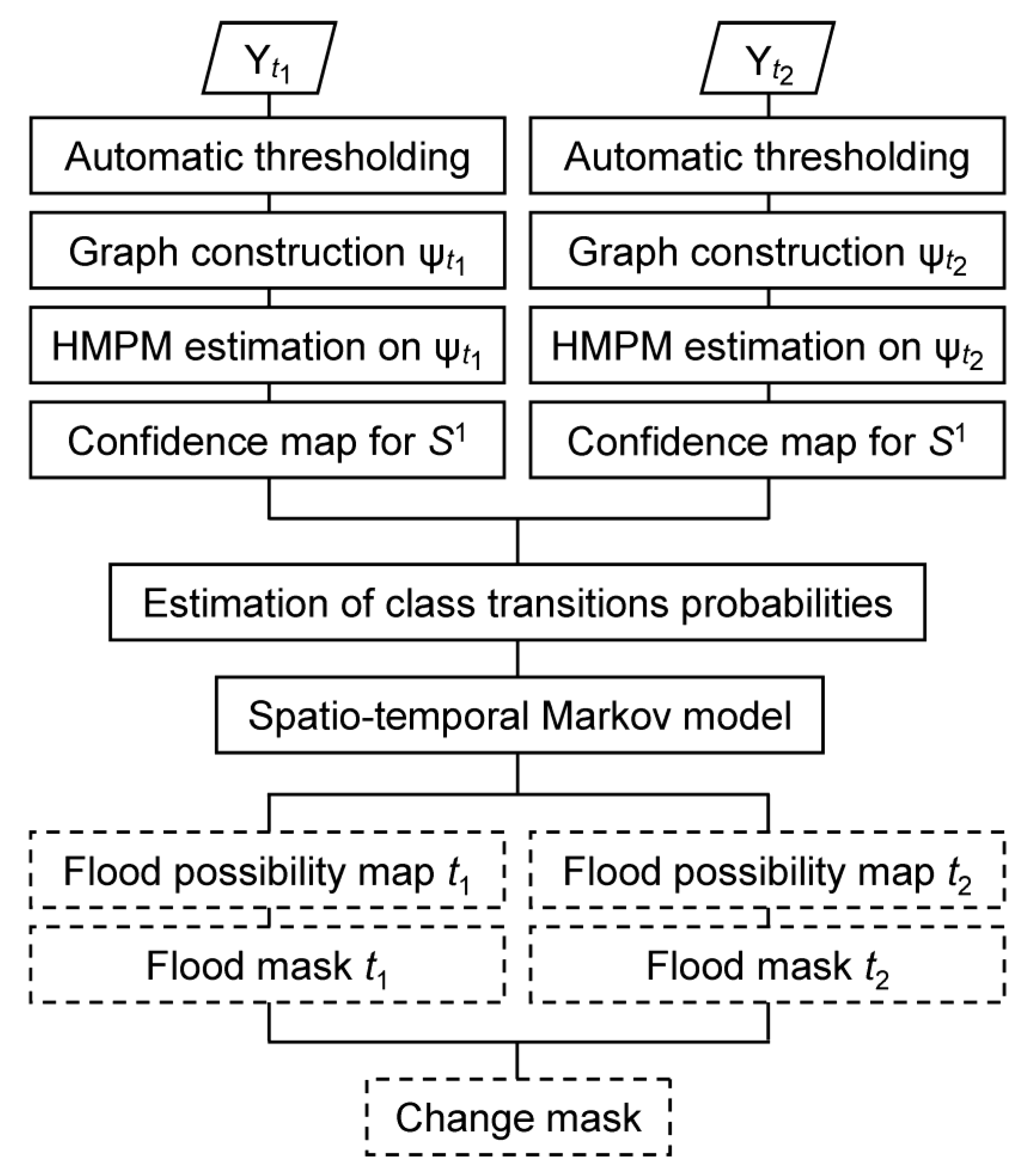
2. Methodology
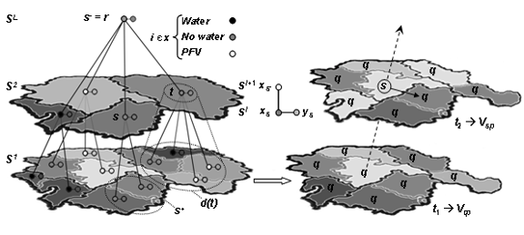
2.1. Automatic Graph Construction

2.2. Markov Image Modeling
2.2.1. Causal Markov Modeling on Irregular Graphs
Problem Definition and Statistical Modeling
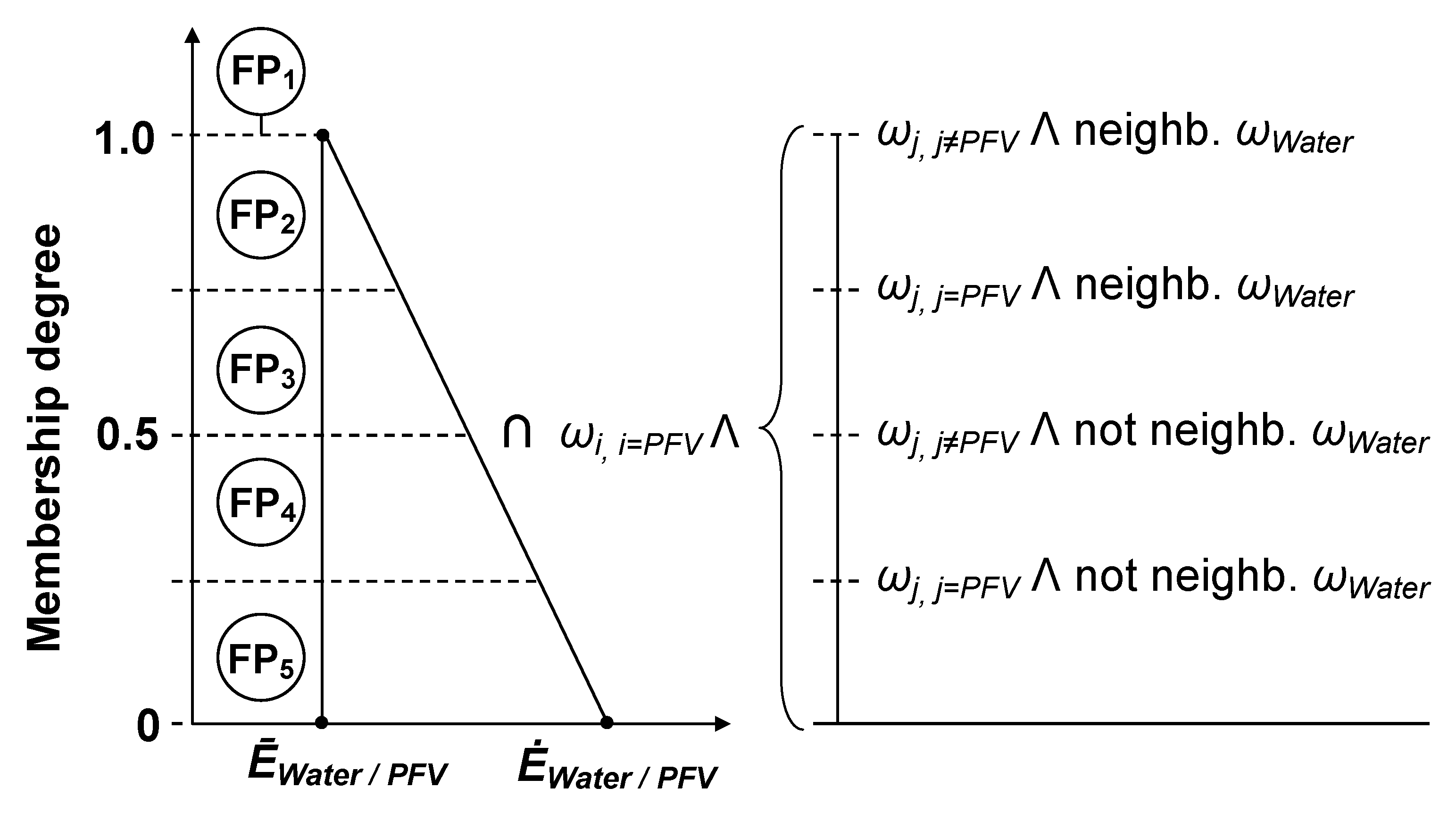
Model Parameters
Inference

| Preliminary pass: At this downward recursion, the marginal priors P(xs) are computed for each s: |
| Bottom-up sweep: The distribution of each xs and couple (xs, xs-) given all the data of the descendants (incl. ys) is provided: |
| Initialization (s∈S1): |
| Recursion (s∈S2… SL): |
| Top-down sweep: The complete marginal posteriors are reassembled from the partial marginals computed at the bottom-up sweep: |
| Initialization (r): |
| Recursion (s∈ SL-1… S1): |
2.2.2 Noncausal Markov Modeling on Bi-Temporal Planar Graphs
Spatio-Temporal Markov Model
Estimation of Temporal Transition Probabilities
2.2.3. Hybrid Multi-Contextual Markov Model
2.3. Generation of Flood Probability Maps
3. Experimental Results
3.1. Data-set Description
3.2. Results and Discussion
| Regular (R-) | Irregular (I-) | |||||||||||
|---|---|---|---|---|---|---|---|---|---|---|---|---|
| T-ICM | HMAP | HMPM | HMAP-ICM | HMPM-ICM | HMAP-w | HMPM-w | HMAP-ICM-w | HMPM-ICM-w | HMAP-ICM | HMPM-ICM | Mean | |
| t1 | 79.90 | 77.08 | 78.50 | 77.62 | 80.30 | 77.80 | 79.67 | 80.39 | 82.97 | 78.63 | 81.78 | 79.5 |
| t2 | 79.77 | 73.80 | 76.97 | 78.11 | 81.04 | 76.23 | 80.86 | 82.48 | 86.33 | 80.07 | 85.20 | 80.1 |
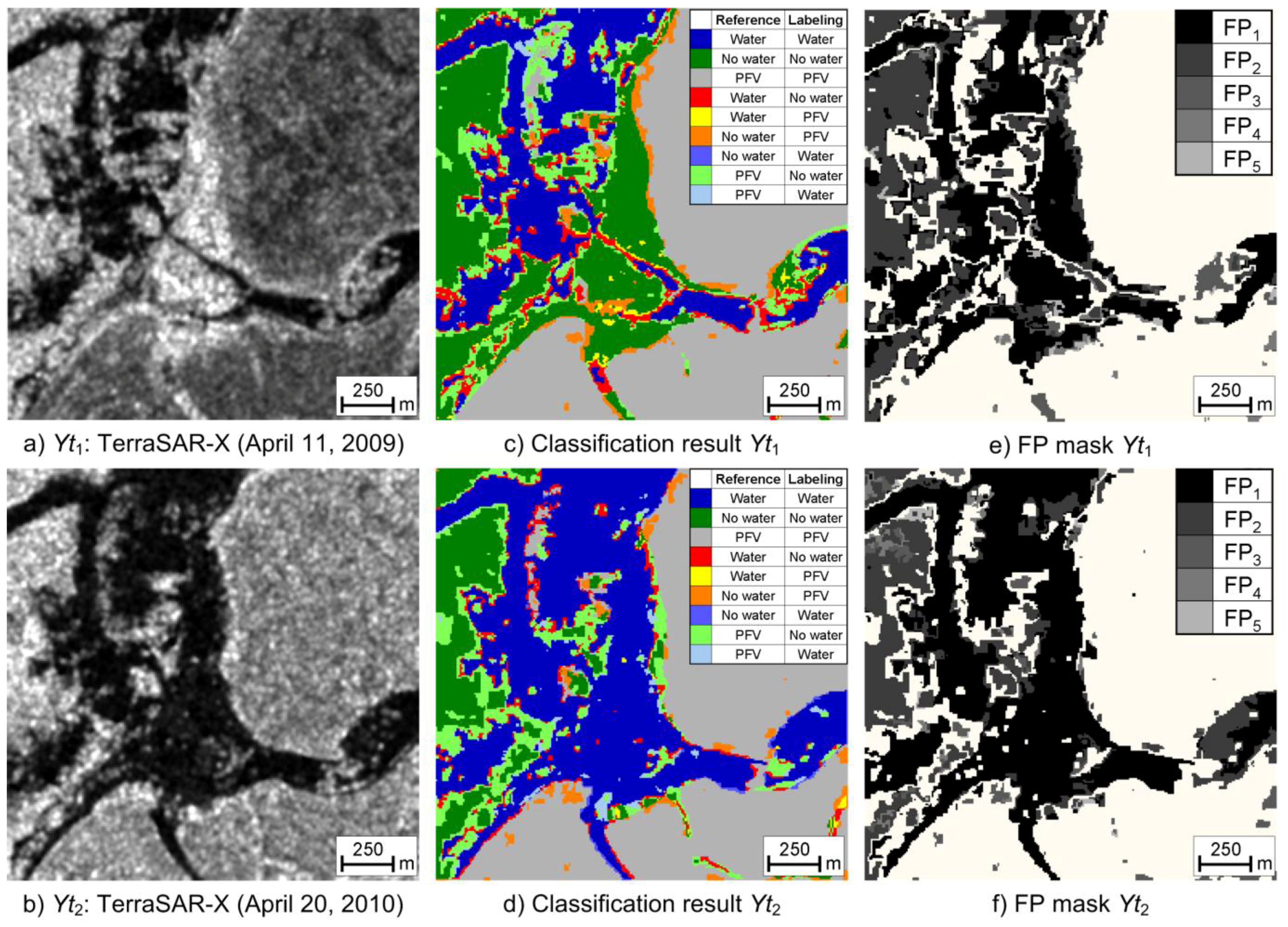
| Reference | ||||||
| Date | Classified | Water | No water | PFV | UA [%] | |
| T1 | Water | 11129 | 2857 | 115 | 14101 | 78.92 |
| No water | 541 | 30261 | 1895 | 32697 | 92.54 | |
| PFV | 236 | 5511 | 12991 | 18738 | 69.32 | |
| 11906 | 38629 | 15001 | 65536 | |||
| PA [%] | 93.47 | 78.33 | 86.60 | OA [%] | 82.97 | |
| Khat [%] | 71.69 | |||||
| T2 | Water | 21240 | 1486 | 61 | 22787 | 93.21 |
| No water | 145 | 29673 | 1546 | 31364 | 94.61 | |
| PFV | 744 | 4976 | 5665 | 11385 | 49.67 | |
| 21610 | 38038 | 5888 | 65536 | |||
| PA [%] | 95.98 | 82.18 | 77.90 | OA [%] | 86.33 | |
| Khat [%] | 77.20 | |||||
4. Conclusion
Acknowledgements
References
- Ormsby, J.P.; Blanchard, B.J.; Blanchard, A.J. Detection of lowland flooding using active microwave systems. Photogramm. Eng. Remote Sens. 1985, 51, 317–328. [Google Scholar]
- Alsdorf, D.E.; Melack, J.M.; Dunne, T.; Mertes, L.A.K.; Hess, L.L.; Smith, L.C. Interferometric radar measurements of water level changes on the Amazon flood plain. Nature 2000, 404, 174–177. [Google Scholar] [CrossRef] [PubMed]
- Horrit, M.S.; Mason, D.C.; Cobby, D.M.; Davenport, I.J.; Bates, P. Waterline mapping in flooded vegetation from airborne SAR imagery. Remote Sens. Environ. 2003, 85, 271–281. [Google Scholar] [CrossRef]
- Lu, D.; Mausel, P.; Brindizio, E.; Moran, E. Change detection techniques. Int. J. Remote Sens. 2004, 25, 2365–2407. [Google Scholar] [CrossRef]
- Mas, J.F. Monitoring land-cover changes: A comparison of change detection techniques. Int. J. Remote Sens. 1999, 20, 139–152. [Google Scholar] [CrossRef]
- Bruzzone, L.; Prieto, D.F. Automatic analysis of the difference image for unsupervised change detection. IEEE Trans. Geosci. Remote Sens. 2000, 38, 1171–1182. [Google Scholar] [CrossRef]
- Martinis, S.; Twele, A.; Voigt, S. Unsupervised extraction of flood-induced backscatter changes in SAR data using Markov image modeling on irregular graphs. IEEE Trans. Geosci. Remote Sens. 2010, 48. Accepted. [Google Scholar] [CrossRef]
- Moser, G.; Serpico, S.B. Generalized minimum-error thresholding for unsupervised change detection from SAR amplitude imagery. IEEE Trans. Geosci. Remote Sens. 2006, 44, 2972–2982. [Google Scholar] [CrossRef]
- Bruzzone, L.; Prieto, D.F. An adaptive semiparametric and context-based approach to unsupervised change detection in multitemporal remote-sensing images. IEEE Trans. Image Process. 2002, 11, 452–466. [Google Scholar] [CrossRef] [PubMed]
- Singh, A. Digital change detection techniques using remotely-sensed data. Int. J. Remote Sens. 1989, 10, 989–1003. [Google Scholar] [CrossRef]
- Melgani, F.; Serpico, S.B. A Markov random field approach to spatio-temporal contextual image classification. IEEE Trans. Geosci. Remote Sens. 2003, 41, 2478–2487. [Google Scholar] [CrossRef]
- Feitosa, R.Q.; Costa, G.; Mota, G.L.A.; Pakzad, K.; Costa, C.O. Cascade multitemporal classification based on fuzzy Markov chains. ISPRS J. Photogramm. Remote Sens. 2009, 64, 159–170. [Google Scholar] [CrossRef]
- Geman, S.; Geman, D. Stochastic relaxation, Gibbs distributions and the Bayesian restoration of images. IEEE Trans.Pattern Anal. Mach. Intell. 1984, 6, 721–741. [Google Scholar] [CrossRef] [PubMed]
- Li, S.Z. Markov Random Field Modeling in Image Analysis, 3rd ed.; Springer-Verlag: London, UK, 2009. [Google Scholar]
- Carincotte, C.; Derrode, S.; Bourennane, S. Unsupervised change detection on SAR images using fuzzy hidden Markov chains. IEEE Trans. Geosci. Remote Sens. 2006, 44, 432–441. [Google Scholar] [CrossRef]
- Benedek, C.; Szirányi, T. Change detection in optical aerial images by a multilayer conditional mixed Markov model. IEEE Trans. Geosci. Remote Sens. 2009, 47, 3416–3430. [Google Scholar] [CrossRef]
- Mota, G.L.A.; Feitosa, R.Q.; Coutinho, H.L.C.; Liedtke, C.E.; Müller, S.; Pakzad, K.; Meirelles, M.S.P. Multitemporal fuzzy classification model based on class transition possibilities. ISPRS J. Photogramm. Remote Sens. 2007, 62, 186–200. [Google Scholar] [CrossRef]
- Solberg, H.S.; Taxt, T.; Jain, A.K. A Markov random field model for classification of multisource satellite imagery. IEEE Trans. Geosci. Remote Sens. 1996, 34, 100–113. [Google Scholar] [CrossRef]
- Liu, D.; Song, K.; Townshend, J.; Gong, P. Using local transition probability models in Markov random fields for forest change detection. Remote Sens. Environ. 2008, 112, 2222–2231. [Google Scholar] [CrossRef]
- Smits, P.; Dellepiane, S. Synthetic aperture radar image segmentation by a detail preserving Markov random field approach. IEEE Trans. Geosci. Remote Sens. 1997, 35, 844–857. [Google Scholar] [CrossRef]
- Jackson, Q.; Landgrebe, D. Adaptive Bayesian contextual classification based on Markov random fields. IEEE Trans. Geosci. Remote Sens. 2002, 40, 2454–2463. [Google Scholar] [CrossRef]
- Kasetkasem, T.; Varshney, K.V. An image change detection algorithm based on Markov random field models. Canad. J. Remote Sens. 2002, 40, 1815–1823. [Google Scholar] [CrossRef]
- Fjørtoft, R.; Delignon, Y.; Pieczynski, W.; Sigelle, M.; Tupin, F. Unsupervised classification of radar images using hidden Markov chains and hidden Markov random fields. IEEE Trans. Geosci. Remote Sens. 2003, 41, 675–686. [Google Scholar] [CrossRef]
- Kasetkasem, T.; Arora, M.K.; Varshney, P.K. Super-resolution land cover mapping using a Markov random field based approach. Remote Sens. Environ. 2005, 96, 302–314. [Google Scholar] [CrossRef]
- Tso, B.; Olsen, R.C. Combining spectral and spatial information into hidden Markov models for unsupervised image classification. Int. J. Remote Sens. 2005, 26, 2113–2133. [Google Scholar] [CrossRef]
- Bouman, C.; Shapiro, M. A multiscale image model for Bayesian image segmentation. IEEE Trans. Image Process. 1994, 3, 162–177. [Google Scholar] [CrossRef] [PubMed]
- Laferté, J.M.; Pérez, P.; Heitz, F. Discrete Markov image modeling and inference on the quadtree. IEEE Trans. Image Process. 2000, 9, 390–404. [Google Scholar] [CrossRef] [PubMed]
- Pérez, P.; Chardin, A.; Laferté, J.M. Noniterative manipulation of discrete energy-based models for image analysis. Pattern Recog. 2000, 33, 573–586. [Google Scholar] [CrossRef]
- Cheng, H.; Bouman, C. Multiscale Bayesian segmentation using a trainable context model. IEEE Trans. Image Process. 2001, 10, 511–525. [Google Scholar] [CrossRef] [PubMed]
- Collet, C.; Murtagh, F. Multiband segmentation based on a hierarchical Markov model. Pattern Recognit 2004, 37, 2337–2347. [Google Scholar] [CrossRef]
- Provost, J.-N.; Collet, C.; Rostaing, P.; Pérez, P.; Bouthemy, P. Hierarchical Markovian segmentation of multispectral images for the reconstruction of water depth maps. Comput. Vis. Image Underst. 2004, 93, 155–174. [Google Scholar] [CrossRef]
- Kato, Z.; Zerubia, J.; Berthod, M. A hierarchical Markov random field model and multi-temperature annealing for parallel image classification. Graph. Models Image Process 1996, 58, 18–37. [Google Scholar] [CrossRef]
- Katartzis, A.; Vanhamel, I.; Sahli, H. A hierarchical Markovian model for multiscale region-based classification of vector-valued images. IEEE Trans. Geosci. Remote Sens. 2005, 43, 548–558. [Google Scholar] [CrossRef]
- eCognition Developer 8 User Guide; Definiens AG: Munich, Germany, 2009.
- Martinis, S.; Twele, A.; Voigt, S. Towards operational near real-time flood detection using a split-based automatic thresholding procedure on high resolution TerraSAR-X data. Nat. Hazards. Earth Syst. Sci. 2009, 9, 303–314. [Google Scholar] [CrossRef]
- Kittler, J.; Illingworth, J. Minimum error thresholding. Pattern Recog. 1986, 19, 41–47. [Google Scholar] [CrossRef]
- Bazi, Y.; Bruzzone, L.; Melgani, F. An unsupervised approach based on the generalized Gaussian model to automatic change detection in multitemporal SAR images. IEEE Trans. Geosci. Remote Sens. 2005, 43, 874–887. [Google Scholar] [CrossRef]
- Forney, G.D. The Viterbi algorithm. IEEE Proc. 1973, 61, 268–278. [Google Scholar] [CrossRef]
- Baum, L.; Petrie, T.; Soules, G.; Weiss, N. A maximization technique occurring in the statistical analysis of probabilistic functions of Markov chains. IEEE Ann. Math. Stat. 2005, 41, 164–171. [Google Scholar] [CrossRef]
- Swain, P.H. Bayesian classification in a time-varying environment. IEEE Trans. Syst. Man Cybern. 1978, 8, 879–833. [Google Scholar]
- Besag, J. Spatial interaction and the statistical analysis of lattice systems. J. R. Stat. Soc. Ser. B 1974, 36, 192–236. [Google Scholar]
- Besag, J. On the statistical analysis of dirty pictures. J. R. Stat. Soc. Ser. B 1986, 48, 259–302. [Google Scholar] [CrossRef]
- Bruzzone, L.; Serpico, S.B. An iterative technique for the detection of land-cover transitions in multispectral remote sensing images. IEEE Trans. Geosci. Remote Sens. 1997, 35, 858–867. [Google Scholar] [CrossRef]
- Bruzzone, L.; Prieto, D.F.; Serpico, S.B. A neural-statistical approach to multitemporal and multisource remote-sensing image classification. IEEE Trans. Geosci. Remote Sens. 1999, 37, 1350–1359. [Google Scholar] [CrossRef]
- Granville, V.; Rasson, J.P. Multivariate discriminant analysis and maximum penalized likelihood density estimation. J. R. Stat. Soc. Ser. B 1995, 57, 501–517. [Google Scholar]
- Feng, X.; Williams, C.K.I.; Felderhof, S.N. Combining belief networks and neural networks for scene segmentation. IEEE Trans. Pattern Anal. Mach. Intell. 2002, 24, 467–483. [Google Scholar] [CrossRef]
- Schumann, G.; Baldassarre, G.D.; Paul, P.D. The utility of spaceborne radar to render flood inundation maps based on multialgorithm ensembles. IEEE Trans. Geosci. Remote Sens. 2009, 47, 2801–2807. [Google Scholar] [CrossRef]
- Richards, J.A.; Woodgate, P.W.; Skidmore, A.K. An explanation of enhanced radar backscattering from flooded forests. Int. J. Remote Sens. 1987, 8, 1093–1100. [Google Scholar] [CrossRef]
- Hong, S.-H.; Wdowinski, S.; Kim, S.-W. Evaluation of TerraSAR-X observations for wetland InSAR application. IEEE Trans. Geosci. Remote Sens. 2010, 48, 864–873. [Google Scholar] [CrossRef]
- Mason, D.C.; Horritt, M.S.; Dall’Amico, J.T.; Scott, T.R.; Bates, P.D. Improving river flood extent delineation from synthetic aperture radar using airborne laser altimetry. IEEE Trans. Geosci. Remote Sens. 2007, 45, 3932–3943. [Google Scholar]
© 2010 by the authors; licensee MDPI, Basel, Switzerland. This article is an open access article distributed under the terms and conditions of the Creative Commons Attribution license (http://creativecommons.org/licenses/by/3.0/).
Share and Cite
Martinis, S.; Twele, A. A Hierarchical Spatio-Temporal Markov Model for Improved Flood Mapping Using Multi-Temporal X-Band SAR Data. Remote Sens. 2010, 2, 2240-2258. https://doi.org/10.3390/rs2092240
Martinis S, Twele A. A Hierarchical Spatio-Temporal Markov Model for Improved Flood Mapping Using Multi-Temporal X-Band SAR Data. Remote Sensing. 2010; 2(9):2240-2258. https://doi.org/10.3390/rs2092240
Chicago/Turabian StyleMartinis, Sandro, and André Twele. 2010. "A Hierarchical Spatio-Temporal Markov Model for Improved Flood Mapping Using Multi-Temporal X-Band SAR Data" Remote Sensing 2, no. 9: 2240-2258. https://doi.org/10.3390/rs2092240