Article

Static Calibration and Analysis of the Velodyne HDL-64E S2 for High Accuracy Mobile Scanning

1
Terrapoint USA Inc, 25216 Grogans Park Drive, The Woodlands, TX 77380, USA
2
Department of Geomatics Engineering, The University of Calgary, 2500 University Drive NW, T2N 1N4, Calgary, AB, Canada
*
Author to whom correspondence should be addressed.
Remote Sens. 2010, 2(6), 1610-1624; https://doi.org/10.3390/rs2061610
Submission received: 7 June 2010 / Revised: 17 June 2010 / Accepted: 18 June 2010 / Published: 22 June 2010

Abstract

:
The static calibration and analysis of the Velodyne HDL-64E S2 scanning LiDAR system is presented and analyzed. The mathematical model for measurements for the HDL-64E S2 scanner is derived and discussed. A planar feature based least squares adjustment approach is presented and utilized in a minimally constrained network in order to derive an optimal solution for the laser’s internal calibration parameters. Finally, the results of the adjustment along with a detailed examination of the adjustment residuals are given. A three-fold improvement in the planar misclosure residual RMSE over the standard factory calibration model was achieved by the proposed calibration. Results also suggest that there may still be some unmodelled distortions in the range measurements from the scanner. However, despite this, the overall precision of the adjusted laser scanner data appears to make it a viable choice for high accuracy mobile scanning applications.

Graphical Abstract

1. Introduction

In the past five years mobile terrestrial scanning has emerged as a suitable tool for performing linear and urban-area surveys of high accuracy. To date, most systems used for mobile scanning are centered around high accuracy 2D line scanners which provide a full 360 degree field of view, such as the Riegl VQ-250, or Optech Lynx. The scanners suffer from a shortcoming that they only are able to view objects in a single plane. Therefore, for multiple look angles, and for occlusion minimization, most systems employ 2 or more of these 2D circular line scanners. In general, they are fairly expensive and can therefore make the use of a mobile terrestrial scanning system quite cost prohibitive.
An attractive alternative to the circular 2D line scanners, both in terms of price and scanning geometry, is the Velodyne HDL-64E S2 scanner. This unit consists of 64 2D line scanners contained within one very compact sensor pod. The 64 lasers are spread out over a 27° vertical field of view (FOV), and the entire unit rotates to give a full 360° by 27° FOV. Up until recently, the Velodyne has been mostly used in autonomous vehicle applications, such as the DARPA Grand Challenge [1]. Recently however, the unit has also emerged in the mobile mapping and surveying market. An overview of the specifications for the Velodyne scanner is given in Table 1, and a picture of the scanner head is given in Figure 1.
Table 1. Manufacturer Specifications for the HDL-64E S2 Scanner [2].
Sensor64 lasers
360° (azimuth) by 26.8° (vertical) FOV
range: 50 m (10% reflectivity) 120 m (80%)
1.5 cm range accuracy (1 sigma)
0.09° Horizontal Encoder Resolution
>1.3333 MHz
LaserClass 1
905 nm wavelength
5 nanosecond pulse
2.0 mrad beam divergence
Figure 1. The Velodyne HDL-64E S2 Scanner.
Remotesensing 02 01610 g001
The adoption of the HDL-64E S2 into the mobile mapping marketplace has occurred without, to the authors’ knowledge, a detailed analysis of system calibration and accuracy achievable with the sensor. High precision mobile mapping applications, such as those for State Departments of Transportation (DOTs) require vertical accuracies better than 1 inch (2.5 cm), see for example [3]. To reliably expect this level of accuracy for mobile mapping applications, a complete understanding of the noise level of the laser scanner is required so that overall expected mobile mapping system accuracy can be evaluated, see for example [4].

2. Mathematical Model of the HDL-64E S2 Scanner

Each of the 64 lasers in the HDL-64E S2 unit is individually aimed and, thus, each has a unique set of calibration parameters. An ideal system can be envisioned as follows. The bundle of rays emanating from the 64 lasers lies in a vertical plane and intersects at the origin of the local scanner coordinate frame. The origin of the range measurement for each laser is located at the scanner origin. The manufacturer defines the following set of parameters for each laser to model the deviations from these ideal conditions:
1. Horizontal Rotation Correction, β. The horizontal angular offset of the laser from the scanner encoder zero angle measured about the z-axis;
2. Vertical Rotation Correction, δ. The vertical angular offset of the laser from the scanner’s xy plane;
3. Horizontal Offset, H. The offset of laser measurement origin from z-axis in the xy plane;
4. Vertical Offset, V. The offset of the laser measurement origin orthogonal to the xy-plane; and
5. Distance Offset, D. Distance bias for each individual laser.
Each of these parameters is illustrated in Figure 2. They are determined by the manufacturer and provided to the end user along with instructions and sample source code to apply the calibration values to the raw measurements in order to reference measurements from all lasers to the local scanner coordinate frame. This set of calibration parameters has been augmented with a linear scale factor after preliminary testing revealed a range dependent error. The computation of local scanner coordinates (x, y, z) for laser i of the Velodyne scanner is given by:
[ x y z ] = [ ( s i *R i + D o i ) * cos ( δ i ) * [ sin ( ε ) * cos ( β i ) cos ( ε ) * sin ( β i ) ] H o i * [ cos ( ε ) * cos ( β i ) + sin ( ε ) * sin ( β i ) ] ( s i *R i + D o i ) * cos ( δ i ) * [ cos ( ε ) * cos ( β i ) + sin ( ε ) * sin ( β i ) ] + H o i * [ sin ( ε ) * cos ( β i ) cos ( ε ) * sin ( β i ) ] ( s i *R i + D o i ) * sin ( δ i ) + V o i ]
where:
si
is the distance scale factor for laser i;
D o i
is the distance offset for laser i;
δi
is the vertical rotation correction for laser i;
βi
is the horizontal rotation correction for laser i;
H o i
is the horizontal offset from scanner frame origin for laser i;
V o i
is the vertical offset from scanner frame origin for laser i;
Ri
is the raw distance measurement from laser i;
ε
is the encoder angle measurement.
Figure 2. (a) Scanner frame axes. (b) Scanner layout. (c) Scanner Parameters in Vertical Plane. (d) Scanner Parameters in Horizontal Plane.
Remotesensing 02 01610 g002

3. Calibration Models

3.1. Mathematical Model for Calibration Adjustment

A variety of approaches have been taken to improve upon the calibration parameters of a laser scanner in order to refine overall measurement accuracy. The adaptation of a photogrammetric calibration approach to terrestrial laser scanners is quite natural and can fairly easily be implemented. This approach is utilized in [5] and [6] for example. Both of these studies use an indoor calibration field that contains a number of targets that can be readily identified in the laser scanner point cloud. The calibration field was observed from a number of different stations, and then a bundle adjustment was performed to simultaneously solve for the scanner orientation parameters, object point coordinates and the internal calibration parameters of the scanner. The instruments used in both studies were tripod-mounted terrestrial scanners which allowed the user to set the horizontal and vertical angular resolutions of the acquired point clouds. With this approach, a fine sample spacing between measured points could be realized, which allows the easy identification of targets in the point cloud.
The HDL-64E S2 however presents a unique challenge. Because the laser was designed for mobile applications, the angular resolution of the output point cloud cannot be modified to provide fine point spacing for signalizing of individual point targets. In fact, this scanner has a fixed vertical angle separation between lasers of 0.3° to 0.5° (5–9 mm at 10 m range) which is much too coarse to allow reliable target measurement. Therefore, a different adjustment approach was required for this scanner. Rather than modeling individual target points, a feature-based approach was chosen. In the current software, planar features are used as the targeted objects, however, the model can easily be changed to model other common features found in LiDAR point clouds.

3.2. Static Plane-Based Functional Model

A plane-based approach for calibration has been implemented in [7,8,9] for calculation of boresight angles for an airborne LiDAR system. Some preliminary investigations for calibrating static terrestrial scanners with a planar approach are also given in [10]. The planar observational model is based upon conditioning the global frame LiDAR points to lie on planar surfaces. In the adjustment model the coefficients of the planes are estimated along with the scanner position, orientation and system calibration parameters. The functional model for conditioning the points can be expressed as:
g k , [ r 1 ] = 0
where g k = [ g 1 g 2 g 3 g 4 ] T are the a priori unknowns of a plane k on which the LiDAR points are conditioned, and r is the vector of globally referenced LiDAR points. In a static calibration scenario, scan data are normally collected from a number of different scan locations, j, and therefore, the ith point can be calculated in a global coordinate frame via a rigid body transformation of the form:
r = R ( w , p , k ) j l i j + t j
where R ( w , p , k ) and t j are the rotational transformation matrix and translation vector between the jth scanner space and the global coordinate frame respectively, and l i j is the scanner space coordinates of point i, given by Equation (1).

3.3. Least Squares Solution for the Static Model

The optimal solution to the least squares adjustment for the functional model described in Section 3.2 is given by the standard Gauss-Helmert adjustment model, which is detailed in [11]. A detailed explanation of the Gauss-Helmert adjustment model which is used to minimize the deviations of the individual LiDAR points from the planar constraints given by Equation (2), is given in for example, [8] or [10] and is therefore not repeated here.
The HDL-64E S2 scanner provides two observations for each laser point, the laser range, and the horizontal encoder angle. The functional model for the scanner, given in Equation (1), infers that there are potentially 6 unknown parameters per laser scanner source in the HDL-64E S2 scanner head. The scan data collected (detailed in Section 4), was captured at unknown station locations. Therefore, the unknown parameters must be expanded to include the unknown scanner translation and rotation parameters into the global reference frame (6 unknowns per scan location). In addition, since no targets with known a priori locations were observed, the scan network must also be constrained. If a scalar distance unknown is not included for the lasers, then the network can be minimally constrained by holding the position and orientation of one scan location fixed. However, in the case of the HDL-64E S2, a distance dependent scale factor was also estimated for each laser. Therefore, in order to constrain the network scale, the position of one additional scan location was also held fixed. A more detailed discussion of network constraints can be found in [12]. Finally, a unit-length constraint must also be added to the system of equations for the direction cosine terms ( g 1 g 2 g 3 ) of each plane.
In examining the mathematical model for the laser, it becomes evident that not all 64 angular offsets can be estimated simultaneously in the adjustment. Only 63 of these parameters are actually independent. Therefore, for the purposes of the adjustment, the horizontal and vertical rotation corrections for the first laser were held fixed. In addition, following the same reasoning, the horizontal and vertical offsets for laser one were also held fixed. Therefore only a distance offset and a distance scale parameter were estimated for the first laser.
With the above assumptions and conditions, and considering I points from S scanner set-ups located on P planar surfaces, the basic quantities of the least squares adjustment are summarized in Table 2.
Table 2. Summary of self-calibration adjustment quantities.
# of Conditionsm = I
# of Unknownsu = 6 * (S − 1) − 3 + 6 * (Lasers − 1) + 2 + 4P
# of Observationsn = 2I
# of Constraintsc = P
# of Degrees of Freedomr = I − u + c

4. Experimental Description

4.1. Data Collection

The static datasets collected for analysis were captured within a courtyard between four identical buildings. Sixteen individual scans were collected from two scanning locations. In each location, data were collected at 0°, 90°, 180°, and 270° azimuth with the laser approximately horizontal. The laser scanner was then tilted by 30°, and data was captured again at the four azimuth values. A schematic drawing of the calibration site and scanner locations as well as an image of one of the buildings in the courtyard is given in Figure 3.
Figure 3. (a) Calibration Site (Buildings in Red, Wood Fence in Green, Scan Locations in Blue). (b) Photo of Building in Northwest Quadrant of Site.
Remotesensing 02 01610 g003

5. Analysis of Results

5.1. Planar Surface Misclosure

As an overall measurement of the improvement the adjusted parameters provided to the laser internal calibration, the misclosure vectors on the planar surfaces used in the adjustment were calculated before and after the adjustment. In both calculations identical station position and orientation values were used to ensure that any differences in the residuals were solely due to the changes in the laser’s internal calibration parameters. A plot of the planar misclosures before and after adjustment is shown in Figure 4, and statistics on the misclosures are given in Table 3.
Figure 4. (a) Planar Misclosure Before Adjustment. (b) Planar Misclosure After Adjustment.
Remotesensing 02 01610 g004
Table 3. Misclosures Statistics Before and After Adjustment.
(meters)Planar Misclosure
BeforeAfter
Min−0.225−0.063
Max0.1480.063
Mean0.0000.000
RMSE0.0360.013
Examination of the results in Figure 4 and Table 3 shows a very marked improvement in the overall precision of the Velodyne laser scanner as a result of the calibration. The RMSE of the misclosures is reduced by almost a factor of three. In addition the systematic trends evident in the planar misclosures before adjustment are almost totally removed by the calibration. The final misclosures do not exhibit any apparent systematic trends.

5.2. Measurement Residual Analysis

In addition to examining the overall improvement in the planar misclosure, it is also instructive to examine the measurement residuals from the adjustment. For the Velodyne laser, there are two measurements per point, a range and an encoder angle. 
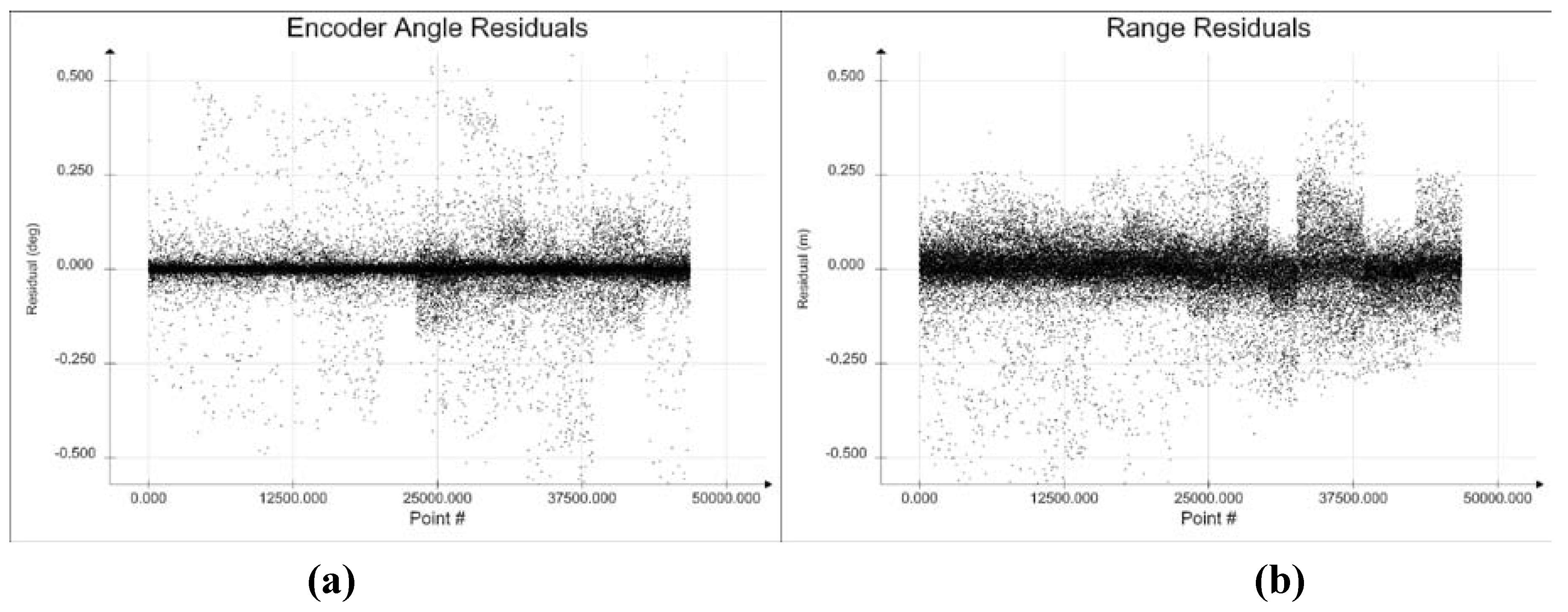
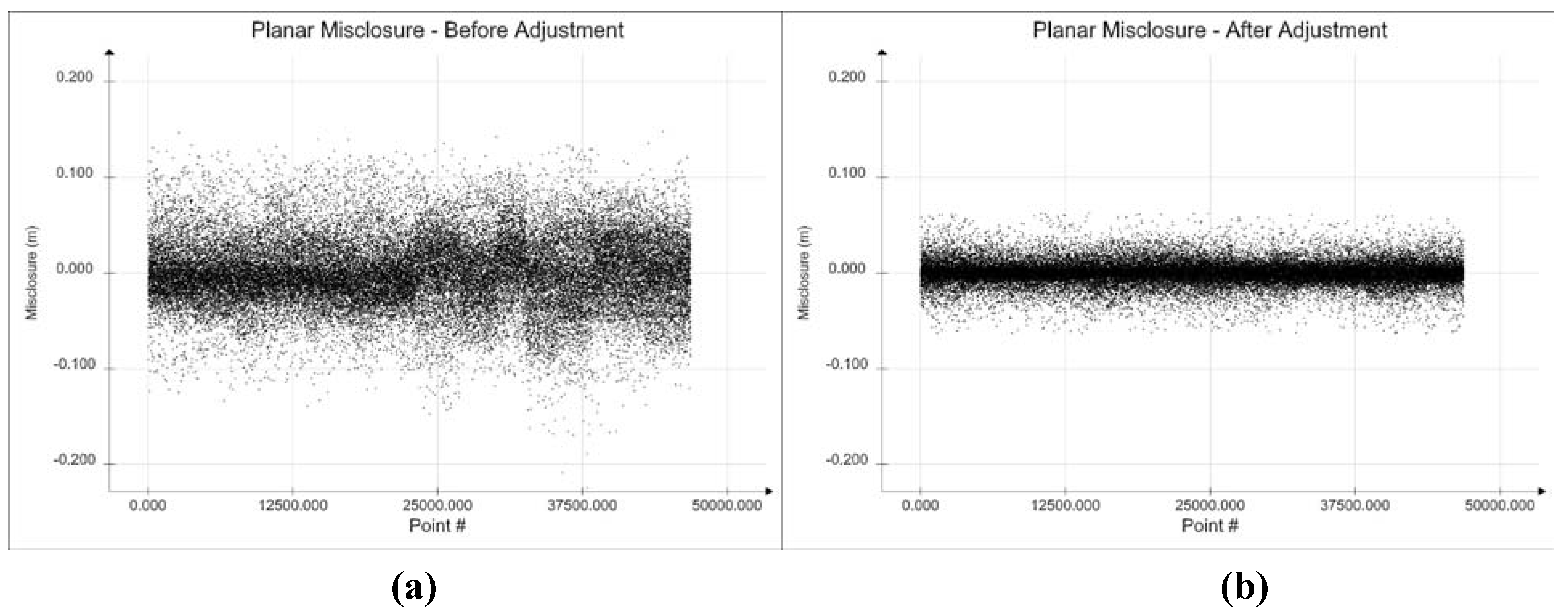
Figure 5 shows plots of the final measurement residuals for the least squares adjustment for both range and encoder angles.
Figure 5. (a) Encoder Angle Residuals. (b) Range Residuals for Least Squares Adjustment.
Remotesensing 02 01610 g005
Figure 5 shows that there are still some unmodelled systematic effects since the range and encoder angle residuals do not appear to be normally-distributed random errors. To further examine these apparent systematic errors, the residuals are plotted in 
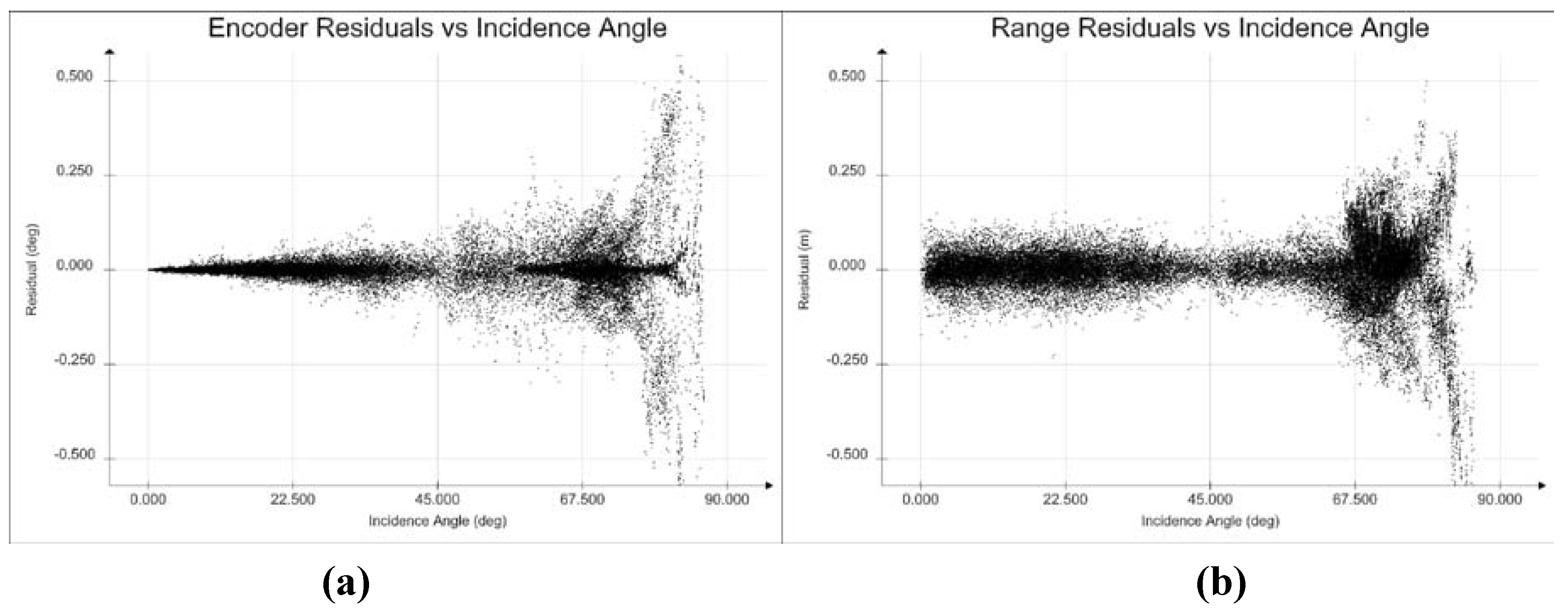
Figure 6 with respect to the laser beam incidence angle on the planar surface. Please note that for all figures, no post adjustment outlier removal procedure has been performed.
Figure 6. Residuals Versus Planar Incidence Angle (a) Encoder Angle (b) Range.
Remotesensing 02 01610 g006
In examining the residuals for the range measurements in Figure 6, the overall noise level and distribution of the residuals appears fairly consistent and regular up to an incidence angle of approximately 60° to 65°. The encoder angle residuals also show a sharp increase in value at approximately the same incidence angle. These results are consistent with other static scanner adjustments found in literature. For example, [5] showed that for an AM-CW scanner, the larger residuals were nearly always isolated to points with incidence angles greater than 65° or 70°, while [13] found critical angles of 65° to 75° for reflectorless total stations. The slightly lower incidence angle threshold found here may be due to the much larger beam divergence for the Velodyne (2.0 mrad) versus the AM-CW scanner in [5], (0.2 mrad) and the instruments in [13] (0.4 mrad and 1 mrad). This pattern suggests that the calibration procedure should reject points with high incidence angles, or alternatively the weighting of the range and encoder angle measurements should be modified to relax the accuracy of observations at higher angles of incidence.
It should also be noted that the encoder angle residuals presented in Figure 6 do not appear to have a uniform distribution across the incidence angle range from 0° to 60°. The residuals at low incidence angles are much smaller than those at higher incidence. However, this pattern is likely not due to any unmodelled error in the encoder angle. At very low incidence angle, the planar misclosure of a point is dominated by range errors and has very low correlation with the encoder angle. Therefore for lower incidence angle points the calculated encoder angle residuals are smaller.
Finally, it is also instructive to compare the range and encoder angle residuals to the manufacturer specifications for ranging and angular accuracy of the HDL-64E S2. Table 4 displays the residuals of both measurements, for all incidence angles, and for incidence angles less than 65°.
Table 4. Range and Encoder Angle Residuals (All Points and Points With Planar Incidence < 65°).
All MeasurementsIncidence Angle < 65 deg
Range (m)Encoder (deg)Range (m)Encoder (deg)
Minimum−1.058−0.940−0.232−0.298
Maximum0.4980.7100.2040.298
Mean0.001−0.0010.0000.000
RMSE0.0840.0630.0370.027
From Table 1, the manufacturer specifications for the unit give a 1σ value for the range at 15 mm, and an encoder angular resolution at 0.09° (0.026° quantization noise standard deviation). The encoder angle residuals in Table 3 are well below the angular resolution of the encoder, and in fact the RMSE of residuals with constrained incidence angles actually approaches the quantization noise level of the scanner. The RMSE of the range residuals however are significantly higher than the manufacturer’s specification for the lasers. Even with the constrained incidence angles the resultant RMSE of the range residuals is still twice the expected value.
The discrepancy between observed and expected range accuracy is significantly larger than expected. Therefore, the range residuals were more closely examined to discover if there was any correlation between the residuals and any other measureable parameters. Analyses of the residuals as a function of laser return intensity did not reveal any dependencies. In addition, the range residuals did not exhibit any apparent correlation with encoder angle, which would suggest that there isn’t a misalignment between the scanner and encoder axes. 
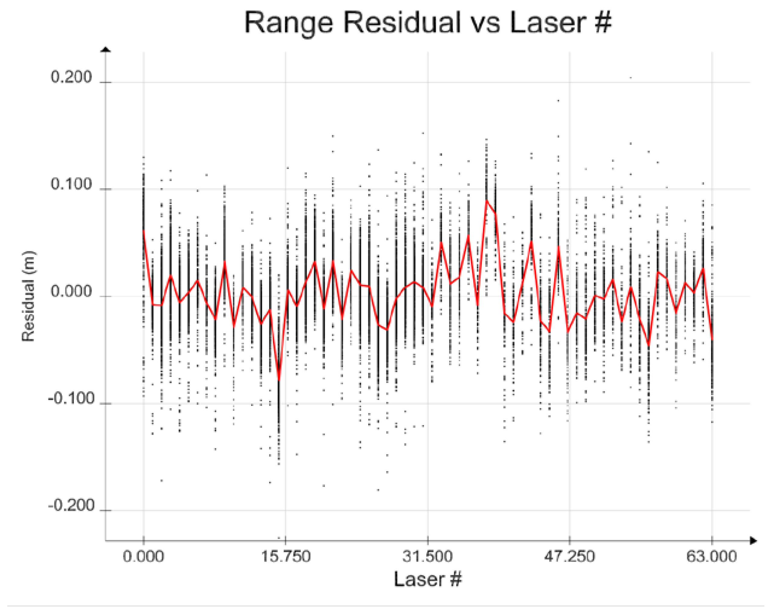
Figure 7 shows range residuals plotted for each individual laser in the 64-laser array excluding observations having planar incidence angles greater than 65°.
Figure 7. Range Residuals versus Laser # (Red Line = Mean Value).
Remotesensing 02 01610 g007
Figure 7 shows what appears to be a systematic error in the ranges. The red line in the figure connects the mean residual values for each laser’s residuals. As is evident from the graph, the lasers do not individually have zero mean residuals. To further investigate this phenomenon, the mean range residuals are plotted in
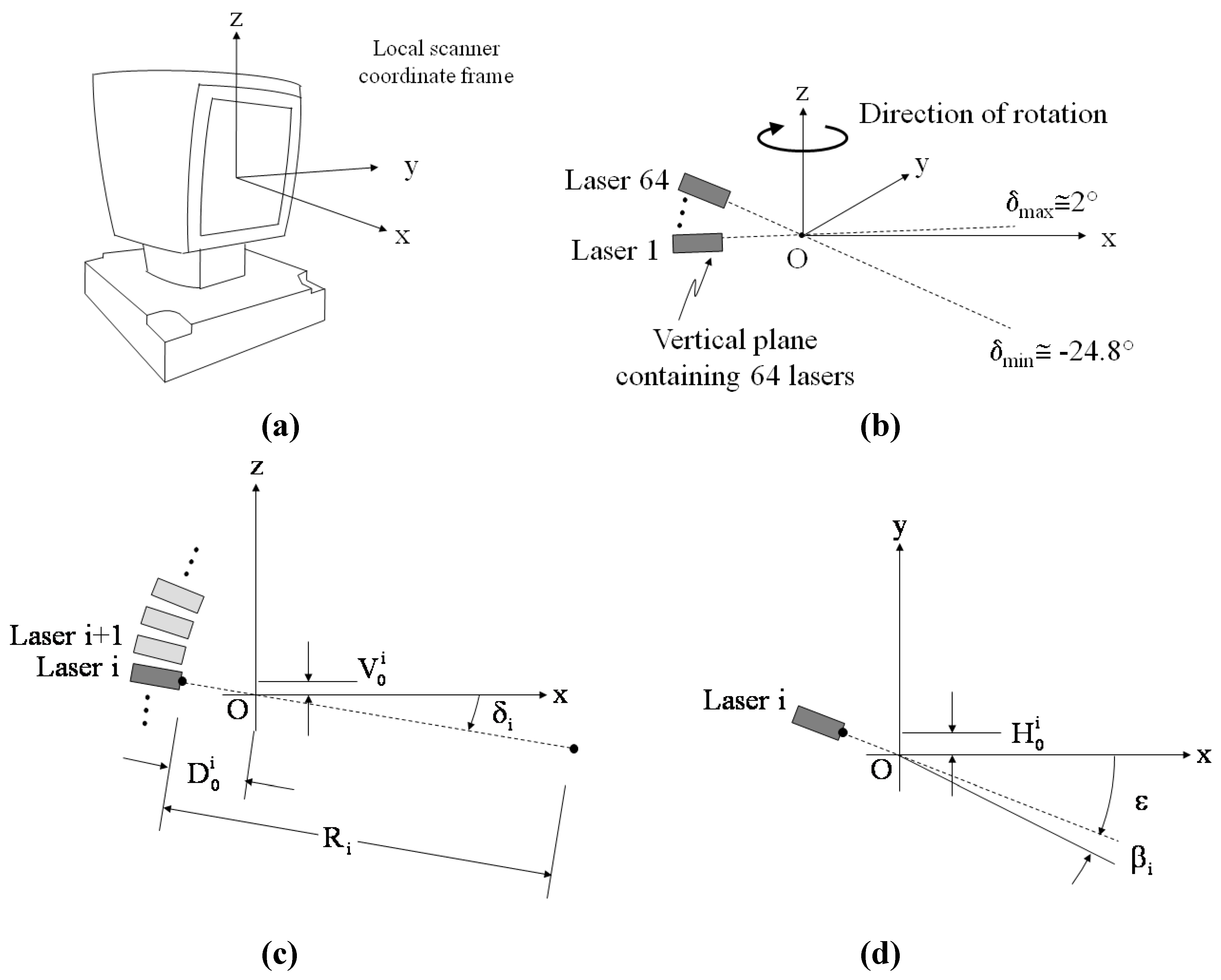
 Figure 8, this time versus the vertical angle, δ, of the laser.
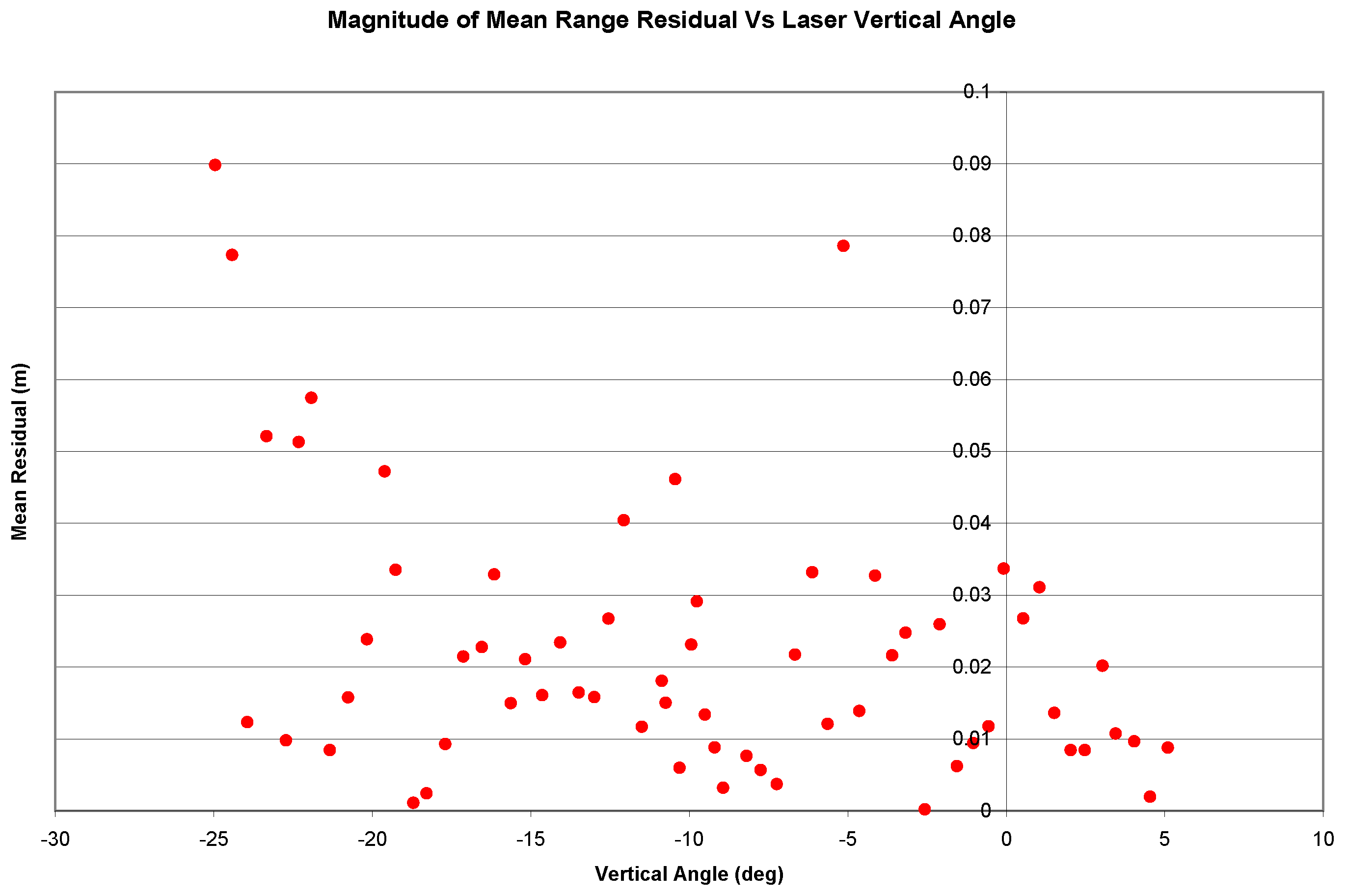
Figure 8. Magnitude of Mean Range Residual vs Laser Vertical Angle.
Remotesensing 02 01610 g008
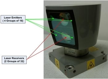
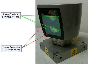
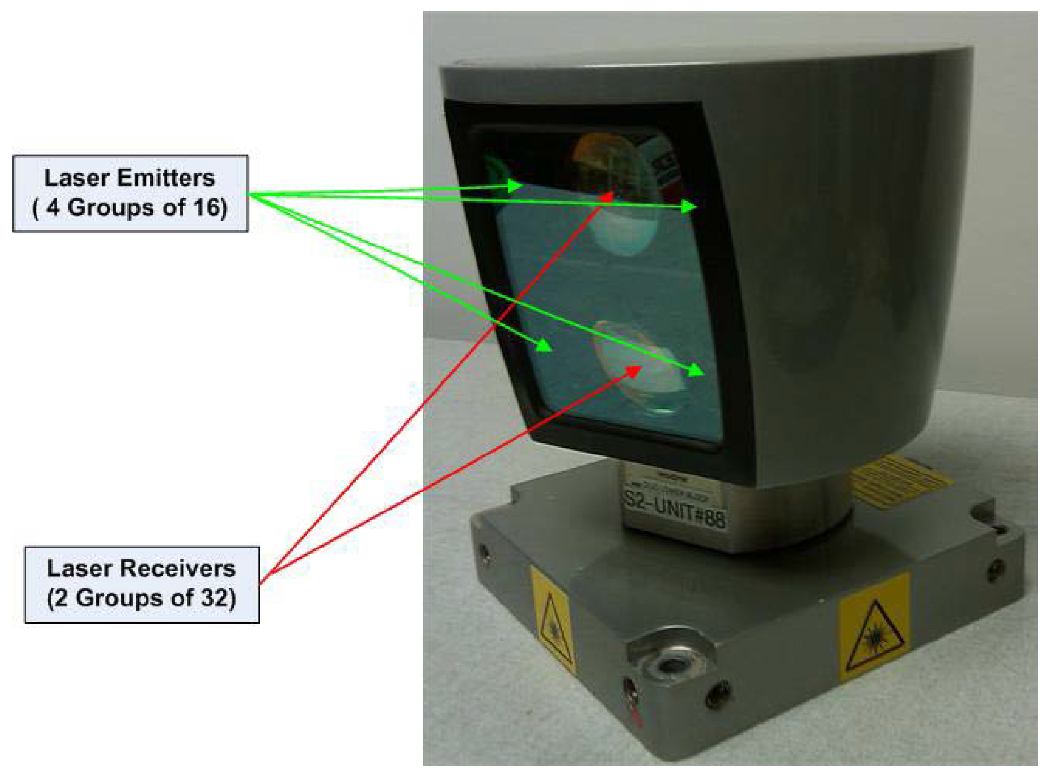
With the exception of one outlier, the mean biases tend to be in the range of 1 to 3 cm, except for a cluster of lasers with the largest vertical angle offsets. In examining Figure 1 it is noted that the lenses for each of the laser emitter and receiver blocks are arranged in order to focus the outgoing laser beams, and to focus the returned energy on the detectors. It is reasonable to assume that the lasers with the highest vertical angle are most likely passing through the emitter and/or receiver mirrors near their edges and are perhaps being distorted in a manner that is not properly modeled by the six coefficients given in Equation (1), or are contributing additional noise to the raw range measurements. This effect will need further study to see if the root cause can be isolated. Nevertheless, even if the five lasers with large mean range residual biases are removed from the computation, the overall RMSE of the range residuals is still only 29 mm (for incidence angles < 65°). This is nearly twice the manufacturer specification. The standard deviations of the individual laser’s ranges however vary between 15 and 25 mm, which is closer to the manufacturer specification, although still slightly higher. It is apparent that there is still an unmodelled component of the laser ranges which is the cause of the non-zero mean residuals, and perhaps for the slightly higher than specification standard deviations.

5.3. Parameter Correlation

A good indication of the strength of the solution and the observability of the individual calibration parameters can be obtained by examining the correlation coefficients between the estimated unknown parameters. Table 5 presents the correlation coefficients for the adjustment. In general, the correlation between the scanner position and orientation parameters between station (e.g., Setup 1 vs. Setup 5) was quite low (<0.1), therefore the light green values in the table are averages over all stations, but only considering correlation with the unknowns from the same station. Similarly, the correlation between the laser parameters of different lasers was quite low (<0.1), and therefore, the values in the grey area of the table are averages over all lasers, but only considering correlation with the other 5 parameters from the same laser. Values in white, correlations between stations and laser unknowns, have been averaged over all stations and all lasers.
Table 5. Correlation Coefficients Between Estimated Unknowns.
Correlation Coefficients
YZOMEGAPHIKAPPADioHioVios
X0.1130.0640.0720.1530.190.0120.0450.0180.0110.0180.029
Yxx0.1140.0710.0830.2270.0230.0150.0220.010.0220.145
Zxxxx0.4590.1950.0420.0380.0130.0390.0140.0350.019
OMEGAxxxxxx0.1570.1880.0980.0170.0250.0210.0940.021
PHIxxxxxxxx0.170.0780.0210.0190.0210.0760.021
KAPPAxxxxxxxxxx0.0220.0680.0230.0240.0180.021
δxxxxxxxxxxxx0.1270.4910.0950.9090.454
βxxxxxxxxxxxxxx0.1320.8790.1110.193
Dioxxxxxxxxxxxxxxxx0.1120.5930.754
Hioxxxxxxxxxxxxxxxxxx0.0910.154
Vioxxxxxxxxxxxxxxxxxxxx0.493
Overall, the station unknown coordinates and orientations exhibit fairly low correlation with themselves, and with the laser unknown parameters. This is to be expected, but also confirms that scanning from unknown locations to targets with unknown absolute locations does not appear to significantly hinder the estimation of the unknown laser parameters.
For the individual laser unknown parameters (grey area in Table 5), the correlation coefficients are in general higher than for the station unknowns. The most troubling are the three correlations highlighted in yellow. The highest correlation, with an average of 0.909, is found between the vertical rotation correction δi, and the vertical offset parameter V o i . The correlation ranges from 0.78 to 0.9 for lasers with a vertical angle between +2° and −12° and from 0.9 to 0.94 for the lasers with larger vertical angles between −12° and −27° degrees. This increase in correlation with increased vertical angle is to be expected because the larger the vertical angle the larger the vertical component of the distance measurement. Although the laser was tilted for 8 of the collected scans, it was only tilted at an angle of 30° with respect to the ground plane. In retrospect, this amount of tilt was likely not enough to completely separate the vertical angle and vertical offset components. This correlation can likely be mitigated in future calibrations by collecting additional data with the scanner tilted 90° (i.e., collecting laser data in a vertical plane), along with the horizontal and elevated scans collected in this study.
The horizontal rotation βi, and horizontal offset H o i , also had a high degree of correlation for the solution, an average of 0.879. The correlation is of approximately the same magnitude for all of the lasers in the scanner array. However, this correlation coefficient increases significantly if the scan stations with 30° of tilt are removed from the solution. Without the tilted scans, this correlation averages 0.94. Therefore, it is reasonable to assume that the addition of scans with the laser tilted at 90° would also help to de-correlate the horizontal rotation and offset components.
Finally, the distance offset, D o i , and distance scale, si, parameters also show fairly high correlation with an average of 0.754. This correlation component varies, and is generally a function of the number of longer ranges observed for the particular laser. The maximum range observed in the calibration dataset was approximately 50 m, and the scale factors for the lasers averaged about 1.0006 (i.e., 3 cm at 50 m), so even at the maximum range the scale factor was still only at the RMSE level of the ranges. Given that the maximum range for the scanners is approximately 125 m, future calibrations should attempt to incorporate longer ranges, up to the scanner maximum, to be able to reliably estimate the scale factor and also decouple it from the distance offset parameter.

5.4. Accuracy of Estimated Parameters

The internal calibration parameters for the laser scanner (and the scanner position and orientation unknowns) were solved for simultaneously in a least square adjustment, and therefore, via error propagation, estimates of the accuracy of the unknown parameters estimated in the adjustment can be calculated. Table 6 presents the maximum, minimum and average correction values for each unknown parameter in the adjustment, along with the average calculated accuracy for that parameter estimate. Given the large number of stations (16), and the large number of lasers (64), an average correction and estimated accuracy was computed for the position and orientation unknowns of the stations, and the 6 laser parameter corrections and estimated accuracies were also averaged over all 64 lasers.
Table 6. Maximum, Minimum and Average Correction and Accuracy Estimates for Unknown Values.
UnknownMaximum
Correction
Minimum
Correction
AverageUnits
CorrectionEstimated Accuracy
X0.0022−0.00140.00070.0012m
Y0.0115−0.00510.00350.0019m
Z0.0004−0.0006−0.00010.0004m
OMEGA0.0133−0.00750.00060.0038deg
PHI0.0058−0.0077−0.00030.0046deg
KAPPA0.0037−0.0068−0.00050.0053deg
V ROT0.3967−0.12990.11180.0124deg
H ROT0.1703−0.1941−0.05170.0167deg
D OFF0.1640−0.01400.06570.0046m
H OFF0.0351−0.0238−0.00060.0039m
V OFF0.0601−0.02030.02230.0028m
D SCALE0.0009−0.0022−0.00060.0003unitless
The results presented in Table 6 have not been scaled by the estimated variance factor for the adjustment. The estimated variance factor was calculated as 6.587. This inflated values is due to the larger than expected noise level of the range measurements as discussed in Section 5.2. Overall the estimated accuracies in Table 6 show an acceptable level of confidence in the estimated parameters. Internal calibration distances are resolved to the order of a few mm, and angular calibration values are resolved to a couple hundredths of a degree—both of which are better than the observed noise levels of the individual range and encoder angle measurements. Therefore, the planar based adjustment procedure utilized seems to give an acceptable level of results and accuracy for calibration of the HDL-64E S2 scanner.

6. Summary and Future Work

A static calibration of the Velodyne HDL-64E S2 laser using a planar feature-based least-squares adjustment was presented and analyzed. Overall, the use of the adjusted laser parameters resulted in a reduction in the planar misclosure RMSE by a factor of almost three over the standard factory calibration model for the scanner. The residuals of the adjustment showed that the noise level of the encoder angle measurements were at or near the quantization noise level of the encoder, if only those measurements with lower incidence angles were considered. The range residuals, however, seemed to indicate that the actual noise level of the range measurements from the scanner was nearer 30 to 35 mm, which is more than double the manufacturer specification. There appears to be some, as of yet, unaccounted for and ummodelled residual systematic noise in the laser ranges. Future work will examine the range residuals to attempt to discover the cause of these unmodelled systematic errors. The unknown parameter estimates showed a higher than expected degree of correlation between the vertical rotation and offset, and the horizontal rotation and offset for each individual laser head. It is felt that in the future additional scan set-ups with the Velodyne elevated into a vertical scanning plane will reduce these correlations. Finally, the high correlation observed between the distance offset and distance scale can be mitigated in the future by increasing the maximum range of observations including in the least squares adjustment.
Overall, however, the results of the adjustment seem quite promising. The planar based least squares approach was able to resolve the internal calibration parameters to an accuracy level that was well below the input observational noise. The final planar misclosure statistics demonstrated that the laser can obtain a 1.3 cm 3D RMS error specification. If this specification can be met under varying conditions and is stable over time, then the HDL-64E S2 scanner has the potential to be an excellent candidate for inclusion on high accuracy mobile mapping platforms. In order to verify this, the temporal stability of the laser in different operating conditions will need to be assessed. Finally, the laser will also need to be integrated into a complete mobile mapping system and undergo testing to determine its overall noise level in a kinematic mapping environment.

Acknowledgments

Velodyne LiDAR is acknowledged for providing the HDL-64E S2 scanner to Terrapoint for analysis for suitability of inclusion in their mobile scanning system solutions. Jerry Dueitt of Terrapoint is also thanked for his assistance in collecting the raw data for the above analysis.

References

  1. Cheung, H. Spinning laser maker is the real winner of the Urban Challenge. TGDaily. 7th November 2007. Available online: http://www.tgdaily.com/trendwatch-features/34750-spinning-laser-maker-is-the-real-winner-of-the-urban-challenge (accessed on May 17, 2010).
  2. High Definition LiDAR; Datasheet for Velodyne HDL-64E S2; Velodyne: Morgan Hill, CA, USA; Available online: http://www.velodyne.com/lidar/products/brochure/HDL64E%20S2%20datasheet_2010_lowres.pdf (accessed on May 28, 2010).
  3. Glennie, C. Kinematic terrestrial light-detection and ranging system for scanning. Transp. Res. Record: J. Transp. Res. Board 2009, 2105, 135–141. [Google Scholar] [CrossRef]
  4. Glennie, C. Rigorous 3D error analysis of kinematic scanning LIDAR systems. J. Appl. Geodesy 2007, 1, 147–157. [Google Scholar] [CrossRef]
  5. Lichti, D. Error modeling, calibration and analysis of an AM-CW terrestrial laser scanner system. ISPRS J. Photogramm. Remote Sensing 2007, 61, 307–324. [Google Scholar] [CrossRef]
  6. Schneider, D. Calibration of a Riegl LMS-420i Based on a Multi-Station Adjustment and a Geometric Model With Additional Parameters. In Proceedings of ISPRS Workshop on Laser Scanning, Paris, France, September 1–2, 2009; pp. 177–182.
  7. Filin, S. Recovery of systematic biases in laser altimetry data using natural surfaces. Photogramm. Eng. Remote Sens. 2003, 69, 1235–1242. [Google Scholar] [CrossRef]
  8. Skaloud, J.; Lichti, D. Rigorous approach to bore-sight self-calibration in airborne laser scanning. ISPRS J. Photogramm. Remote Sensing 2006, 61, 47–59. [Google Scholar] [CrossRef]
  9. Skaloud, J.; Schaer, P. Towards automated LiDAR boresight self-calibration. In Proceedings of 5th International Symposium on Mobile Mapping Technology, Padova, Italy, May 29–31, 2007. [CD-ROM].
  10. Bae, K.H.; Lichti, D. On-site self-calibration using planar features for terrestrial laser scanners. In Proceedings of ISPRS Workshop on Laser Scanning and SilviLaser, Espoo, Finland, September 12–14, 2007. [CD-ROM].
  11. Förstner, W.; Wrobel, B. Mathematical concepts in photogrammetry. In Manual of Photogrammetry, 5th ed.; McGlone, J.C., Mikhail, E.M., Bethel, J., Mullen, R., Eds.; American Society of Photogrammetry and Remote Sensing: Bethesda, MD, USA, 2004; pp. 15–180. [Google Scholar]
  12. Kuang, S. Geodetic Network Analysis and Optimal Design: Concepts and Applications; Ann Arbor Press: Chelsea, MI, USA, 1996. [Google Scholar]
  13. Lichti, D.; Lampard, J. Reflectorless total station self-calibration. Survey Review 2008, 40, 244–259. [Google Scholar] [CrossRef]

