Article

Mapping Bush Encroaching Species by Seasonal Differences in Hyperspectral Imagery

1
Biocentre Klein Flottbek and Botanical Garden, University of Hamburg, Hamburg, Germany
2
German Remote Sensing Data Center, German Aerospace Center, Oberpfaffenhofen, Germany
3
Institute of Photogrammetry and Remote Sensing, Vienna University of Technology, Vienna, Austria
*
Author to whom correspondence should be addressed.
Remote Sens. 2010, 2(6), 1416-1438; https://doi.org/10.3390/rs2061416
Submission received: 15 March 2010 / Revised: 12 April 2010 / Accepted: 19 May 2010 / Published: 27 May 2010
(This article belongs to the Special Issue Ecological Status and Change by Remote Sensing)

Abstract

:
Bush encroachment is a form of land degradation prominent worldwide, but particularly present in semi-arid areas. In this study, we mapped the spatial distribution of the two encroacher species, Acacia mellifera and Acacia reficiens, in Central Namibia, based on their different phenological behavior. We used constrained principal curves to extract a one dimensional gradient of phenological change from two hyperspectral images taken in different seasons. Field measurements of species composition and cover values were statistically related to bi-temporal differences in hyperspectral vegetation indices in a direct gradient analysis. The extracted gradient reflected the relationship between species composition and cover values, and the phenological pattern as captured by the image data. Cover values of four dominant plant species were mapped and species responses along the phenological gradient were interpreted.

Graphical Abstract

1. Introduction

Bush encroachment is a form of land degradation that can be found worldwide [1], but it has been documented for arid and semiarid rangelands much more frequently than for temperate regions [2]. It can be described as an increase in biomass and abundance of woody species and the suppression of perennial grasses and herbs [3]. Although the causes are still debated, there is evidence that effects of poor land management, such as overgrazing by cattle, is a main driver facilitating the spread of encroacher species [4,5]. In water-limited ecosystems, this process might be enforced in the future by altering precipitation patterns as expected through climate change [6].
In semiarid rangelands, bush encroachment leads to dense thickets, often made up of thorny or unpalatable bushes which negatively affect the carrying capacity and thus the economic value of rangelands [4,7]. If bush encroachment occurs, arboricides are often used as a chemical bush control agent, with predominantly negative effects on the environment as well as on the quality of farm products such as meat leaving local markets [8]. Furthermore, plant and animal diversity is negatively affected through a decrease in vegetation structural diversity [9,10,11] leading to an overall loss of ecosystem functioning.
Over the last years, management strategies for the quantification of the encroachment process have largely benefited from remote sensing. Analysis of time series based on aerial photographs [12,13] or satellite imagery [14,15] helped to quantify the encroached area over different time spans. Although the quantification of bush encroached areas has made significant progress at all spatial resolutions, little effort was made in disentangling the spatial patterns of different encroaching species. However, this type of information could help decision makers in applying species-specific management strategies, which are often needed to control the encroaching species successfully [16].
In Africa, species of the genus Acacia often act as encroaching species. For example in Zanzibar, Acacia auriculiformis has been identified as a heavy encroacher [17]. In Botswana, A. tortilis and A. erubescens have been reported to increase in rangelands [18]. In Namibia, Acacia mellifera and Acacia reficiens are among the main encroacher species [16,19]. They belong to the same genus, do not differ in their overall stature, and often occur together in the same habitats. Although both species are shedding their leaves in the dry season, they clearly differ in leaf phenology [20]. While A. mellifera starts with fresh leaves already in September, the first leaves of A. reficiens do not sprout before December.
In general, seasonal phenological changes are mainly caused by inter-annual climatic variability and are reflected through an increase or decrease in green biomass [21]. For remote sensing, phenology provides valuable information for distinguishing vegetation types. For example, Hüttich et al. [22] used phenological differences based on MODIS data to better separate vegetation types with similar life forms. Resasco et al. [23] were able to map an invasive shrub in understorey vegetation based on comparisons of seasonal differences in vegetation indices. In several recent studies, phenological differences in leaf traits [24] and canopy characteristics [25] allowed discrimination of vegetation at the species level based on leaf spectral signatures. In the context of bush encroachment in Namibia, known differences in leaf phenology of the encroacher species could facilitate distinguishing between the two prevailing Acacia species based on multi-temporal remote sensing imagery. However, no spatially explicit mapping of encroacher species has been performed so far.
The aim of the present study is to produce species specific cover value maps that reflect the distribution pattern of two main encroaching bush species in Central Namibia, A. mellifera and A. reficiens, based on their different phenological characteristics. To produce the maps, we will apply a constrained ordination analysis, in order to relate field measurements of species composition and their cover values with bi-temporal differences in hyperspectral vegetation indices. For this purpose, we will extract a one dimensional gradient of phenological change, which is inherent to the difference images of the spectral indices. Based on a statistical relationship between species occurrences and the phenological gradient, a map of phenological change for the study area will be predicted, indicating the distribution of each species.

2. Material and Methods
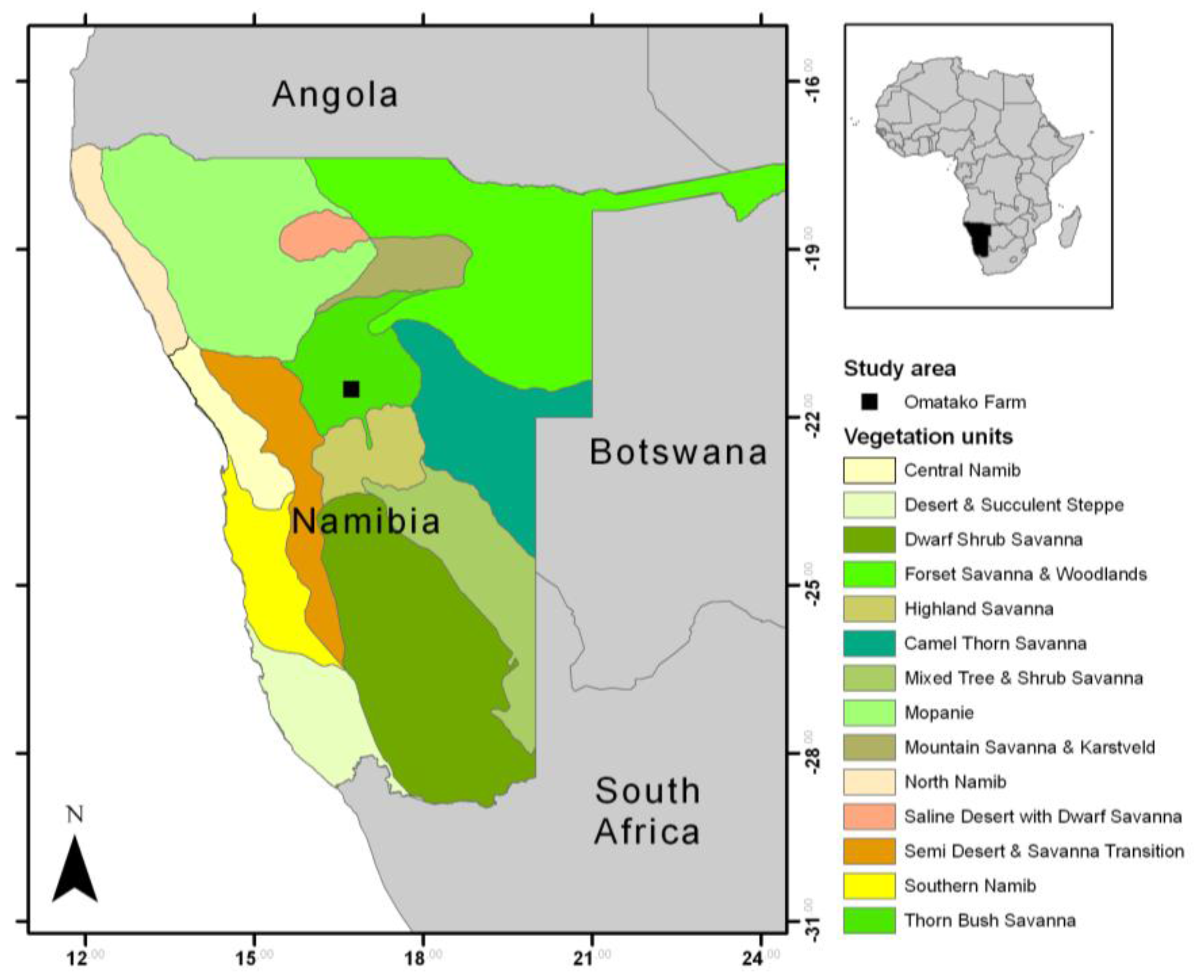
2.1. Study Region

According to the vegetation map of Giess [26], the study area lies in the Thornbush savanna in central Namibia and is situated on the commercial game farm Omatako (Lat: −21.501 Long: 16.729) (Figure 1) comprising an area of about 18 km2. Climate is semi-arid with an average annual rainfall of 300–350 mm. The main rainy season is summer (November–May), but the main rainfall occurs between December and April. Rainfall patterns show a high interannual and spatial variability. The dry season lasts from May to the end of October and often has less than 10 mm rainfall. Vegetation can be characterized as open savanna vegetation with a continuous grass and herb layer and a more or less dense shrub layer. Thorny shrubs, mostly Acacia spp., may form very dense stands with only little understorey growth. On the farm, bush encroachment can be partly explained by grazing effects of the former land use strategy of cattle farming. The main soil types are ferralic cambisols and arenosols, as well as chromatic luvisols [27]; thus, topsoil colors are either more reddish or bright yellow.
Figure 1. Localization of the study area on the Omatako Farm in Central Namibia on top of a vegetation map by Giess [26].
Remotesensing 02 01416 g001

2.2. Vegetation Sampling

We visited the study area three times; in late October 2005, during the dry season, the area was visited in order to observe dry season aspects but no vegetation samples were taken. In April 2006, a field campaign was conducted and 40 vegetation samples were taken. Another field campaign was carried out in April 2007 when 87 samples were taken. At both sampling campaigns, preferential sampling [28] was applied in order to maximize discrimination of different vegetation types. Each vegetation sample consisted of an area of 25 m × 25 m (625 m2), where all vascular plant species were listed and their cover was estimated visually on a percentage scale [29].
Because the sampling years differed considerably in rainfall, vegetation samples were made comparable for both years by deleting all annual species and all species with a cover share of less than five percent of all vegetation samples in the dataset. Otherwise, the difference in species composition between the years would have confounded further multivariate analyses. To prevent biases introduced by a large number of zero cover occurrences or by a small number of very high cover values, the cover values in the species data matrix were transformed using the Hellinger distance [30], which is the square root of the row totals divided by the row mean values. This distance measure showed good performance for abundance data throughout different multivariate ordination methods, especially for those relying on a linear gradient structure [31].

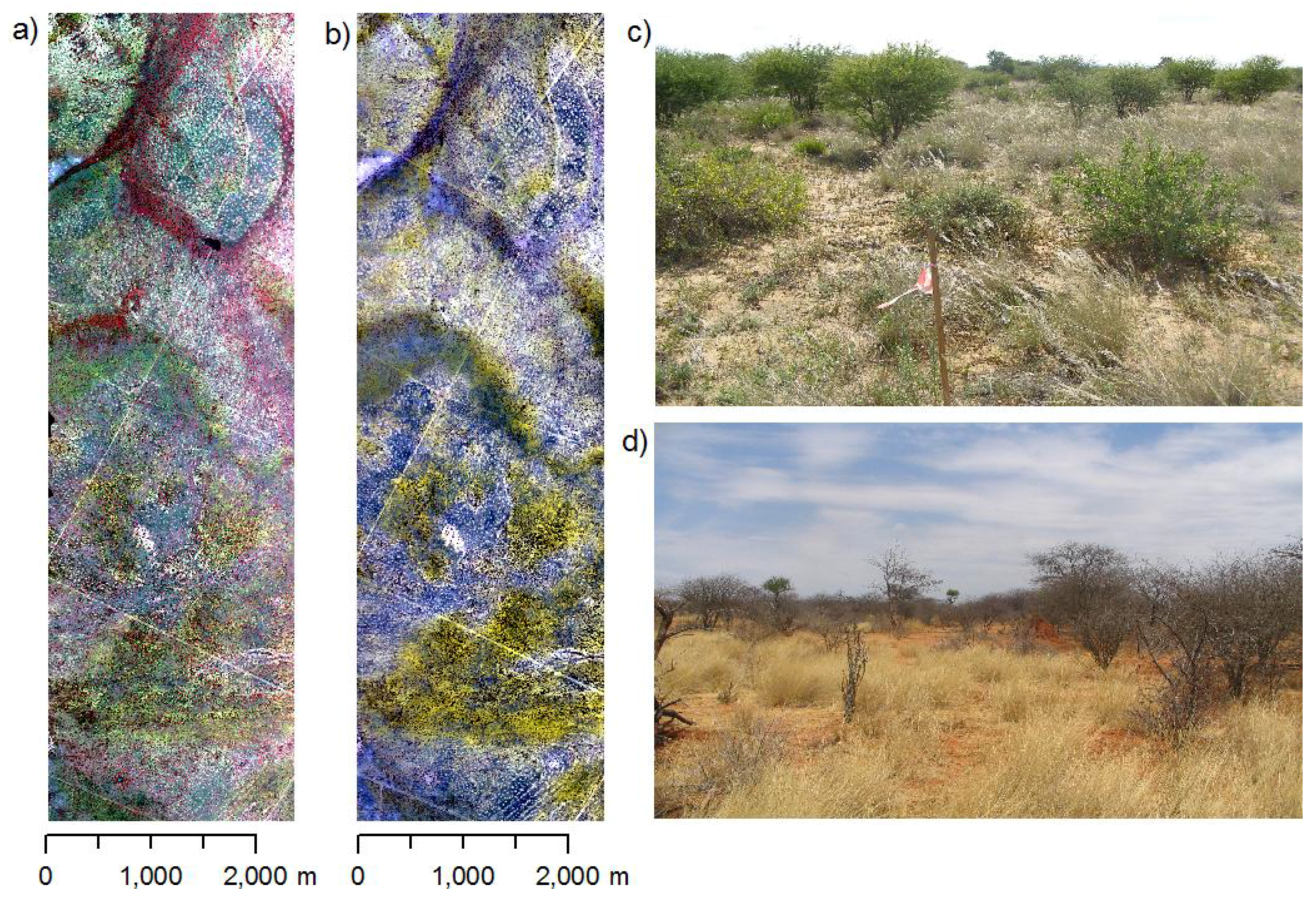
2.3. Image Acquisition

Two hyperspectral images were acquired for the study area. The first acquisition took place at the end of the rainy season in early April 2004 (Figure 2a,c) capturing the vegetation shortly after its maximum greenness. The second image was acquired at the end of the dry season in early November 2005 (Figure 2b,d). Images were taken using the airborne imaging spectrometer HyMap [32]. This sensor measures radiance in 126 bands over the 0.44–2.5 µm spectral region with a spectral bandwidth between 10 and 20 nm. The operational altitude of 3,000 m resulted in a spatial resolution of 5 m. Images were orthorectified using the PARGE software [33] in combination with 15 differential GPS measurements (accuracy ~0.5 m). Errors of the rectified images were less than 1 pixel (<5.0 m) in x- and y-direction. ATCOR-4 [34] was used for vicarious calibration and for the removal of atmospheric effects. For the vicarious calibration, spectroradiometric measurements were taken during the first field campaign in 2005 using a portable Fieldspec PRO FR spectrometer (Analytical Spectral Devices, Inc.) at four homogeneous dark and bright bare soil targets and converted into reflectance units using a Spectralon™ panel as white reference. Depending on wavelength, the deviation of ground measured reflectance and HyMap reflectance obtained after atmospheric correction varied between 1 and 4% absolute reflectance units.
Figure 2. HyMap images and photos from the study area showing the differences between rainy and dry season in the study area. (a) Rainy season image (April, 2004, CIR). (b) Dry season image (October, 2005, CIR). (c) Rainy season vegetation aspect (d) Dry season vegetation aspect.
Remotesensing 02 01416 g002

2.4. Vegetation Index Differencing

Vegetation index differencing, or univariate image differencing, is the most commonly applied change detection technique for analyzing differences between two or more dates [35,36]. Values from the second-date vegetation index are subtracted from the first-date vegetation index on a pixel-by-pixel basis. This algebraic approach is a straightforward method, allowing an easy implementation and interpretation. The resulting image is interpreted in a way that positive values represent a decrease in the values between both time points, whereas negative values represent an increase. Values around zero only show little change between the two time steps. According to Lu et al. [37], two aspects have to be taken into consideration: First, selecting suitable vegetation indices for the purpose of the study, and second, selecting suitable thresholds to identify the changed areas. In our case, the latter point was not necessary, since we did not intend to interpret the differenced images directly, but to use these in a further multivariate analysis.
We selected six different spectral indices (Table 1) according to their different biophysical meaning, their usefulness for savanna ecosystems, and their applicability to hyperspectral data based on previous working experience [38]. Furthermore, only spectral indices were chosen that showed Pearson correlation values below 0.75 with other spectral indices. In order to calculate the difference images, we first calculated the indices for each seasonal image and then subtracted the dry season index images from those of the rainy season. Finally, we extracted the difference index values from each pixel at each vegetation sample (25 m × 25 m) and calculated the mean of the pixel values as a reference for each sample.
Table 1. Overview of the selected vegetation indices and their canopy related feature. For index formulas see Dorigo et al. [39].
Nr.IndexFull nameFeatureReference
1CARIChlorophyll Absorption in Reflectance IndexChlorophyll[40]
2DGVIDerivative Green Vegetation Index (1st order)Greenness[41]
3LWVILeaf Water Vegetation IndexWater[42]
4NDLINormalized Difference Lignin IndexLignin[43]
5NDNINormalized Difference Nitrogen IndexNitrogen[43]
6CAICellulose Absorption IndexCellulose[44]

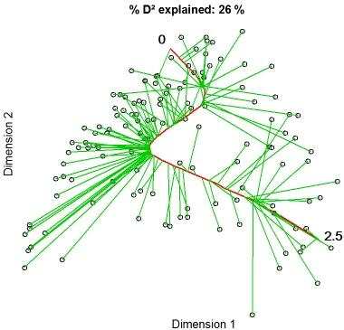
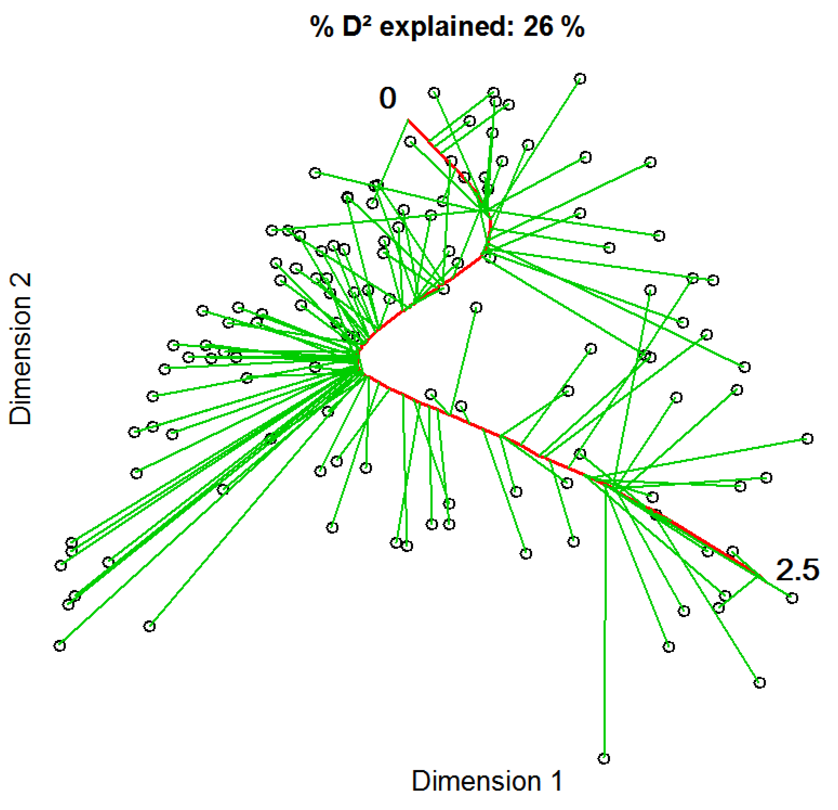
2.5. Constrained Principal Curves

Principal curves can be described as nonlinear generalizations of principal components analysis (PCA), that use nonlinear regression and local smoothers to minimize the sum of squared deviations between the response variable and the fitted curve [45]. Principal curves extract one major underlying gradient from the data itself by passing through the data cloud in an n-dimensional space, where n equals the number of parameters used. This is comparable to an indirect ordination method in ecology that searches for latent gradients in the species data [46]. De’ath [47] extended the indirect ordination method to a constrained form of principal curves, allowing a second matrix to be taken into consideration during curve fitting. Thus, the analysis becomes a direct ordination, comparable to a Canonical Correspondence Analysis (CCA), in which environmental parameters are used to describe a relationship between species and habitat characteristics. In our case, the second matrix hosted the differenced spectral index values.
Principal curves are constructed as follows: at the beginning, an initial projection of the species data in a multivariate space must be defined. The choice of this initial projection is a crucial step, since all later projections will depend on it, and thus the outcome of the final curve. Following recommendations for vegetation data [47], we applied a nonmetric-multidimensional scaling (NMDS) using Bray-Curtis distance on the Hellinger transformed species data. The scores of the first NMDS-axis were used for the initial configuration. The fitting of the curve follows an iterative two-step project-expectation algorithm [48]. First, in a projection step, a straight line is drawn as close to the points as possible. Each point of the curve is then the average of all data points that project to it. In a constrained principal curve analysis, this is the point where the locations of the sites along the curve are linearly regressed on the environmental variables. Hence, the site locations on the final curve can be explained by the parameters of the constraining matrix. The second step is an expectation step, where the straight line is bending to a curve, improving the fit of the curve to the points. These steps are repeated until convergence is reached or until a defined number of iterations have passed. For the algorithm setup, we set the number of iterations to 20 and chose smoothing splines as the curve fitting method. Furthermore, extended dissimilarities with a threshold at 0.75 were chosen for calculating the initial configuration. This improves the relationship between species distance and ecological distance in cases of high beta-diversity [49], i.e., a large species turnover which we expected for the dataset. Principal curves were calculated using the R-package pcurve [50]. All analyses using the pcurve package were carried out in the R-software environment [51].
In order to find a model that best explains the relationship between species cover and seasonal differences in the images, we used a stepwise backward approach, i.e., we recalculated the curve fitting process after iteratively deleting one difference index per step from a full model. We evaluated the models resulting from the stepwise procedure by comparing four criteria: First, we controlled the percentage variance explained by the curve. This is similar to the variance explained by the first axis of a PCA. The model with the highest explained variance was preferred. Second, we investigated the shape of the curve, which is an important curve characteristic. Heavily undulating or intersecting curves imply overfitting, whereas smooth curves with no or only few bends can be interpreted as a reasonable fit. Third, we noted the R2 of the linear model resulting from a regression of the site locations on the environmental variables and finally, we used the Akaike Information Criterion (AIC) [52] for comparing models with different numbers of predictors. AIC is an entropy based information criterion that measures the information loss based on the maximized empirical likelihood [53]. We compared the AIC differences between all candidate models and chose the model with the smallest AIC, indicating a minimal loss of information, i.e. the model with the best statistical fit.

2.6. Mapping and Validation of Plant Species Cover

After the best model was found, we applied the resulting intercept and regression coefficients to the original difference images in order to create an image representing curve locations along the principal curve, i.e., reflecting decreases or increases in the overall phenology. Since the species responses along the principal curve were based on smoothing spline regression, it was possible to calculate cover maps for species within the model. For the four main dominant species (Figure 2) we extracted their respective smoothing spline models from the principal curve model and predicted them onto the new curve location image.
For validation of the species cover maps, we used an external validation dataset which was provided by the BIOTA-Africa project [54]. This project monitors vegetation in the study region on an annual basis since 2000. Once per year, usually in the end of the rainy season when vegetation cover is fully developed, on so called Biodiversity Observatories. The Observatory comprises an area of one square kilometer and is subdivided into 100 one hectare plots. Twenty of these hectare plots were selected randomly. In the centre of each of the selected hectares a 20 m × 50 m and a nested 10 m × 10 m plot were used for annual vegetation monitoring First, we extracted the cover values from our predicted species cover maps for the areas of the BIOTA-vegetation plots, i.e., 4 pixels for the 10 m × 10 m and 40 pixels for the 20 m × 50 m plots. Then, we calculated the mean value of the extracted values, since we can use only one cover value per plot. In order to assess the quality of the species maps, we computed parametric and non-parametric correlation coefficients, i.e., Pearson’s r and Spearman’s r, to validate if there is a linear correlation between the predicted cover values and the measured cover values from the external dataset. Furthermore, we calculated two-tailed probabilities that the values are uncorrelated. From the external dataset, we used observed cover values from two years in which the hyperspectral images were taken, i.e., 2004 and 2005. For the correlation analysis we used the free statistical software PAST [55].

3. Results

3.1. Constrained Principal Curves

We conducted direct gradient analysis using constrained principal curves in order to find nonlinear relationships between vegetation samples and seasonal differences of vegetation indices. The final principal curve explained 26% of the variation in the vegetation data and had a final length of 2.5, measured in arc-length [48] (Figure 3). The curve did not show heavy distortions, but followed a slight z-shape. Most of the samples were grouped in the middle rather close to the curve, but some samples are located at longer distances. At both ends, grouping was less dense and the projected distances from points to the curve seemed to be longer than of those in the middle.
Figure 3. The constrained principal curve, shown in red, is fitted to the initial projection of vegetation samples based on a NMDS using Bray Curtis distance explaining 26% of the variation in the species composition. Green lines represent projection-vectors that connect data points with their respective curve locations. The zero marks the starting point of the principal curve, i.e., the left-hand side, while the 2.5 indicates its end, i.e., the right-hand side of the curve.
Remotesensing 02 01416 g003
In the best performing regression model used for fitting the curve all six variables were significant and linearly related to the locations on the principal curve (Table 2). Although ΔNDLI was only significant at the p = 0.1 level, deleting the variable would have led to a considerably higher AIC value (0.79 instead of 0.69), hence ΔNDLI was kept in the model. Steepest increase of values along the curve was found for ΔLWVI and ΔNDNI, as indicated by their slopes. The final regression model reached a multiple R2 of 0.53. For a better interpretation, the six variables were put into two groups; Right hand side positive (RHS) and left hand side positive (LHS). RHS positive are ΔCAI, ΔDGVI and ΔLWVI, because they were positively related with the curve, i.e., starting with negative values and then steadily increased. The indices in this group are mainly related to canopy greenness. Positive values at the start of the curve characterize indices from the LHS group. These indices are ΔCARI, ΔNDLI and ΔNDNI, which all are mainly related to an increase in non-photosynthetic materials such as twigs, branches, and dry leaves.
Table 2. Regression coefficients of the final partial linear model.
slopeStd. Errort valuep
intercept2.66460.38266.9647<0.001
Δ CARI−3.70140.6685−5.5365<0.001
Δ LWVI38.53999.41534.0933<0.001
Δ CAI10.38214.51462.2997<0.05
Δ NDLI−18.328513.1827−1.3903<0.1
Δ NDNI−32.93895.589−5.8935<0.001
Δ DGVI14.39143.48364.1312<0.001
R2: 0.53, p => 0.001

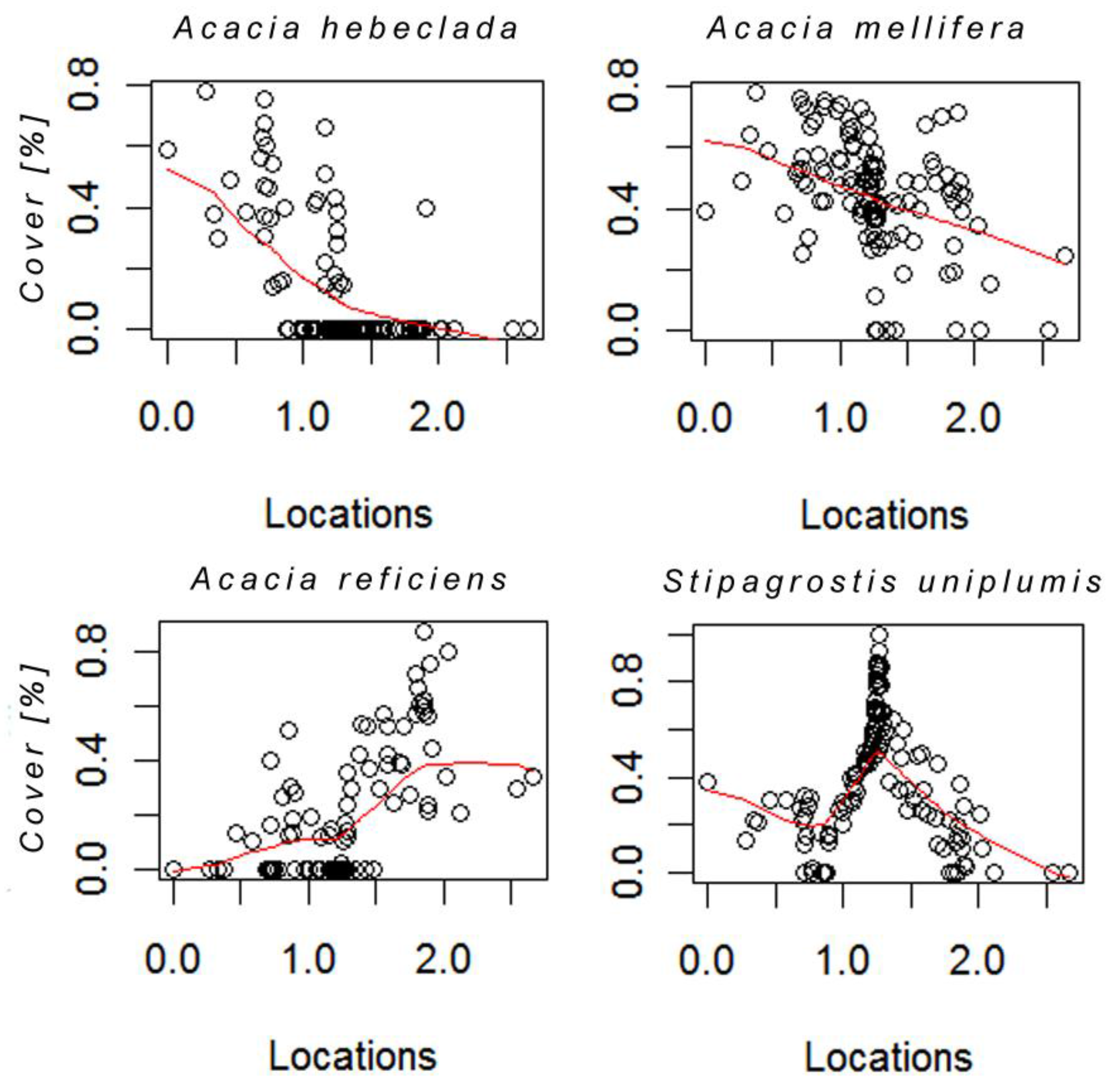
3.2. Species Responses

Species responses along the curve are shown for the four most dominant species in form of nonlinear regression smoothing spline plots (Figure 4). Due to the fact that these species make up most of the cover in the study area, we assume that they also contribute substantially to the spectral signal in the images. Acacia hebeclada and A .mellifera, both perennial shrubs, showed a strong linear decrease from left to right on the curve, both having occurrences of zero cover around the location 1.0 on the principal curve. However, point distribution of A. mellifera indicates that the species occurs throughout the whole curve, yet showing decreasing cover values with increasing location values. In contrast, A. reficiens shows an increase in cover with higher locations on the curve. Zero occurrences are distributed between locations 0 and 1.5. However, the distribution is not strictly linearly increasing due to two plots in which A. reficiens occurs with only moderate cover values. The perennial grass Stipagrostis uniplumis shows a unimodal distribution with an optimum in the middle of the gradient around 1.25. Similar to A. mellifera the species is very common in the study area, as indicated by the few zero occurrences.
Figure 4. Hellinger transformed cover values of four dominant species plotted for each location on the curve. The red line represents the smoothing spline used to fit the individual response shape.
Remotesensing 02 01416 g004

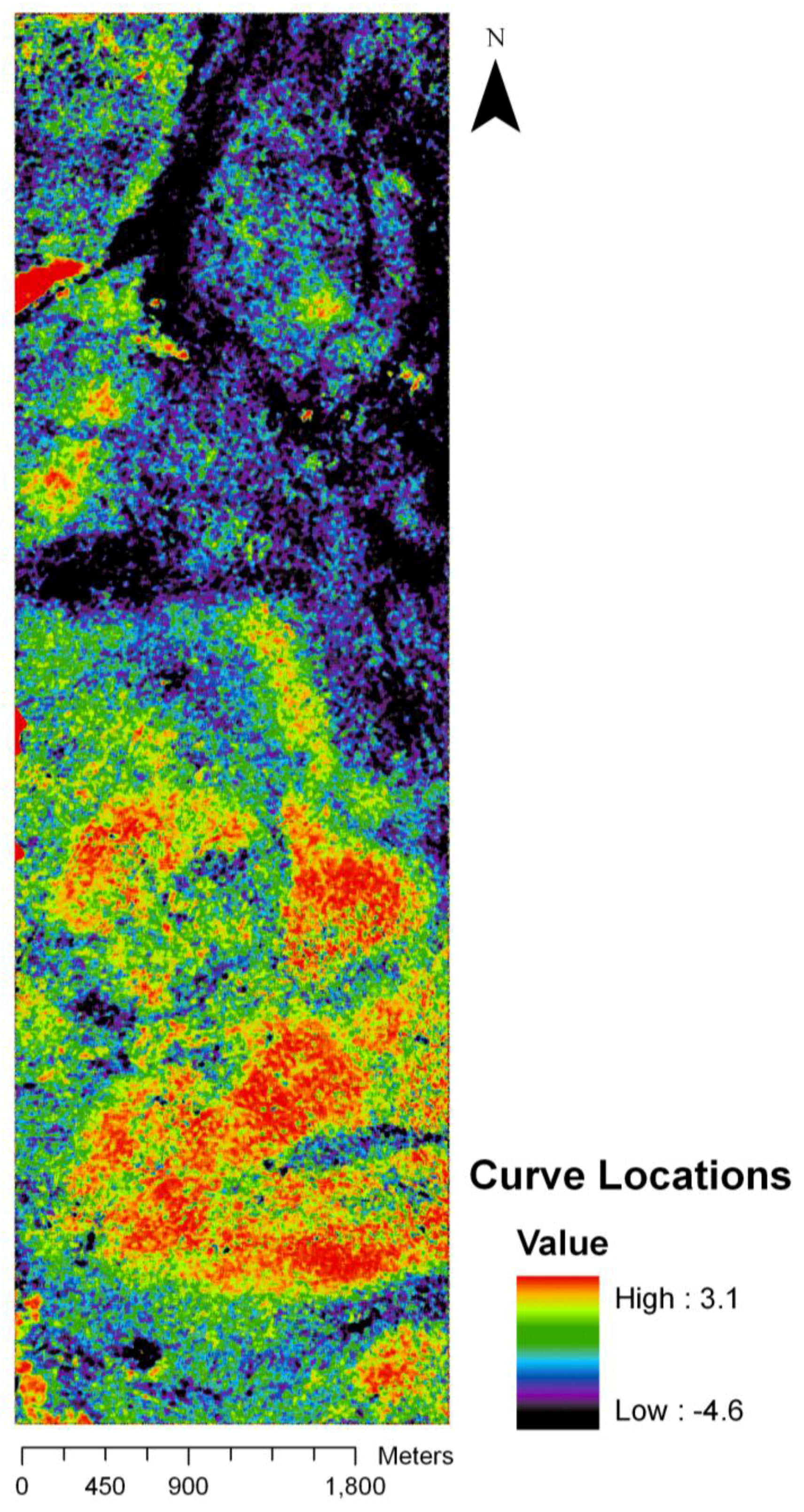
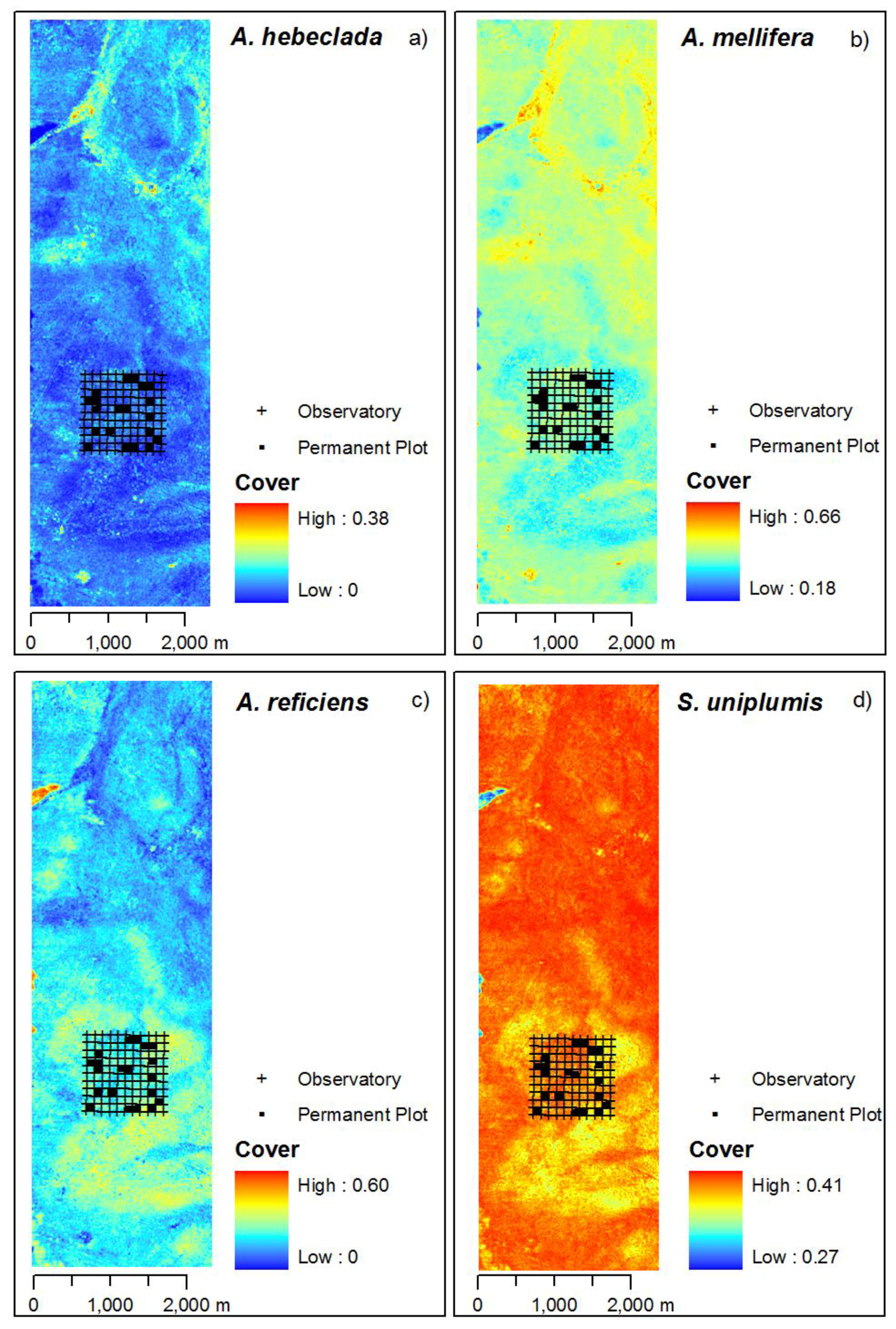
3.3. Mapping of the Principal Curve and Species Cover

The regression coefficients of the final model were used to predict curve locations on the base of the HyMap imagery. This resulted in a new image representing predicted curve location per pixel with values ranging from −4.1 to 3.6, thus extrapolating beyond the original length of the curve (Figure 5). However, very high or low values were only found in few extreme values and did not distort the main spatial pattern. The different colors represent different sections on the curve, going from the left hand side of the curve (black to violet) to the right hand side of the curve (bright green to red). The light blue to dark green colors indicates the central section of the curve. While black and violet colors dominate in the northern part of the image, bright green and reddish colors are more prominent in the southern part. However, one larger spot dark red spot and several smaller are also located in the northern part. The areas showing locations from the central part of the curve (light blue to dark green) appear throughout the image.
Figure 5. Predicted image of curve locations. Continuous colors from black to red represent the phenological change gradient from left to the right hand side of the curve.
Remotesensing 02 01416 g005
Based on the curve location image, we predicted species cover maps using the species specific response model, i.e., the smoothing regression spline (Figure 6). The four plant species show different centres of dominant cover. A. hebeclada and A. mellifera have highest values in the northern part of the study area. A. mellifera is more common throughout the whole study area with values well above zero. A. reficiens occurs throughout the study area overlapping with A. mellifera, yet with a center of dominance in the south of the study area while not occuring close to areas with higher values of A. hebeclada. However, predictions of cover values for A. reficiens show a large range from 0.00 to 0.60. S. uniplumis occurs throughout the whole study area as well, having highest cover values in the north and north-western part of the study area.
Figure 6. Predicted species cover maps of Hellinger-transformed cover values. Included are the positions of the permanent plot monitored by the BIOTA-Africa project, the source of the external validation dataset. Observatory marks the total covered area of 1 km2 by the monitoring design. Images are stretched between minimum and maximum values.
Remotesensing 02 01416 g006

3.4 Validation of Species Cover Maps

We validated the species cover maps by calculating parametric and nonparametric correlations between predicted and observed cover values. The resulting correlation values are presented in Table 3. The cover map for A. hebeclada did not show any significant correlations below 0.05. The A. mellifera cover map showed relatively high correlation values on both plot sizes, except for the non-parametric test on 10 × 10 m. The two-tailed p-values support the correlation coefficients. The A. reficiens cover map performed best in the non-parametric tests, supported by p-levels significant at the 5% level, while no significant correlation was found in the parametric tests. The S. uniplumis cover map showed reasonable Pearson correlation on the 20 m × 50 m plot, however with only a weak support by the two-tailed p-values.
Table 3. External validation of the species cover maps for two plot sizes. The number of plots where a species occurs (n) is given per plot size. Parametric (Pearson) and non-parametric (Spearman) correlation values are shown. The p-value is based on a two-tailed probability test for correlating values. The column ‘year‘ marks the year with the highest correlation values found.
SizeSpeciesnPearson’s rpyearSpearmann’s rpyear
10 × 10A.hebeclada3−0.110.6422004−0.270.2482004
A.mellifera120.540.01420050.210.3752005
A.reficiens90.230.33320050.460.0432004
S.uniplumis200.370.10520050.320.1742005
20 × 50A.hebeclada60.130.59220040.180.4432004
A.mellifera190.450.04720040.450.0492004
A.reficiens170.320.16520050.520.0202005
S.uniplumis200.380.09920040.260.2622005

4. Discussion

4.1. Phenological Gradient

Information on vegetation phenology is increasingly used for distinguishing between vegetation types in remote sensing studies [22,56,57]. In this study, we were able to identify a phenological gradient of change using a constrained principal curve that was fitted to data from a vegetation survey constrained by a set of differenced spectral indices. Spatial distribution patterns of four dominant plant species, including two known bush encroacher species, were identified based on their known phenological differences, i.e., a different onset of shoot growth [20].
The relationship between the extracted principal curve and the spectral indices, as expressed by their regression coefficients in the linear model (Table 1), describes the found phenological pattern. The two identified groups of indices (LHS and RHS) summarize the general phenological trend in the data. Locations situated on the LHS of the curve, have more negative values in greenness related difference indices in the November image (dry season) than in the April image (rainy season). Although there was an overall decrease in greenness in the study area in the beginning of November 2005, canopy greenness at locations on the LHS of the curve is relatively higher than at locations on the RHS. Locations are less green and less moist there, but they have higher values in dry matter lignin and nitrogen. Because of their functional and spectral similarity, cellulose and lignin are often lumped together as dry-matter or nonphotosynthetic vegetation [58]. High values of lignin normally go together with higher values in cellulose due to ageing processes in cell wall structure, which negatively affects digestibility and thus fodder values of vegetation [59,60]. However, in our case, the cellulose absorption index (CAI) is positively related with locations on the curve, in contrast to the NDLI (Table 2). We interpret this contrast as different stages in the lignin-cellulose ratio in the canopy due to phenological differences. This ambiguity might also explain why the regression coefficient of the NDLI is less significant. Locations in the middle of the curve show only little positive or negative change in both directions. To summarize, we can interpret the extracted principal curve as a gradient of phenological change, from mainly fresh-leaf (LHS) to leaf-less (RHS) canopies, and locations on the curve are placed according to the relation between species composition and spectral indices.

4.2. Species Responses

We found that the four major plant species have distinct responses along the phenological gradient. Woody species have high cover values at both ends of the curve, i.e., Acacia mellifera and A. hebeclada are on the LHS, while the abundance of A. reficiens is highest on the RHS of the curve. Stipagrostis uniplumis and many other herbaceous species have highest cover values in the middle of the curve. The location of those species on the curve can be best explained by their phenological behavior. The Namibian Tree Atlas [20] is a valuable source of information on the phenology of many woody species in Namibia. According to the Tree Atlas, A. reficiens does not have any leaves in October and November, which goes along with the trend of decreased greenness, and increased dry-matter content in the November image. This is expressed by the spectral indices that were identified to be positively related with the RHS locations on the curve. In the same time period, A. mellifera and A. hebeclada carry already leaves, and thus are located at the LHS of the curve, going together with a relatively higher amount of greenness in the image.
The effect of leaf shedding on the spectral response can be mainly explained by the change in the amount of visible soil affecting the signal. This seems to be especially true for encroaching species that usually lack a well developed understorey vegetation [11,61]. Species with general high cover values that have no leaves will allow soil signals to be superior to the vegetation signal in the image.
In the middle of the phenological gradient, perennial grasses dominate in cover while Acacias and other larger shrub species occur only in small abundances. Evergreen trees, such as Boscia albitrunca also occur here in larger abundances. We assume that evergreen trees contribute only little if any to changes in the phenology and thus are situated in the middle of the curve. In contrast to the situations at the ends of the curve, here the often discussed tree-grass ratio of savanna ecosystems [62] is shifted towards the herbaceous component. Chidumayo [63] pointed out that the pattern of leaf phenology in savanna vegetation is influenced by the differential leaf phenology between the woody and the herbaceous component. While shoot growth of the woody component is triggered at the end of the dry season, grass growth is restricted to the rainy season due to water availability in the upper soil layer [63,64]. However, not all tree species share the same leaf sprouting rhythm, hence the pattern found in this study confirm the general findings of Archibald and Scholes [64] and the phenological pattern described for the species in the Namibian Tree Atlas [20].
Several studies showed that the leaf-flush of the herbaceous component of savannas considerably increases greenness as measured by spectral indices [63,64]. However, in our study, the vegetation samples with a larger herbaceous component did not strongly change in any spectral index. In 2004, in the beginning of April when the rainy season image (Figure 2a) was taken, grasses had already dried out. Hence, we conclude that greenness of the herbaceous component was already rather similar between dry and rainy season and therefore only little change was found between the two images. Furthermore, perennial grasses do not shed any leaves but remain with their dried standing biomass throughout the dry season, i.e., keeping a constant value of cover. Hence, they always provide a minimum of reflectance leading to higher values in the vegetation indices than in those areas where only leafless A. reficiens without understorey occurs. We conclude that the effect of a dominating perennial grass sward stabilizes the reflectance signal when images from the end of rainy seasons are compared with dry season images by providing a constant, yet drier, vegetation signal. In other words, leaf shedding shrubs without a grass layer in the understorey, often found in bush encroached areas, will provide a higher change in the signal due to the resulting contrast of leaves and soil signals over the seasons.

4.3. Mapped Vegetation Pattern

We created a map of the phenological pattern by predicting the curve locations onto the differenced index images (Figure 5). Interestingly, the right hand side of the curve forms rather broad island-like patterns while values from the left hand side seem to follow a topographic pattern, e.g., a water course. The locations from the center of the curve build the matrix in which the other patterns are embedded. The species cover maps (Figure 6) emphasize species specific patterns. While A. hebeclada seems to be more restricted to specific landscape features, the other three species show broader distribution patterns yet with different centers of dominance. A. mellifera and A. reficiens do partly overlap mainly in the southern parts of the study area. S. uniplumis occurs in the whole study area showing no values below zero, yet with higher values in the northern areas.
How can the different spatial patterns be explained in terms of phenology? We found that A. hebeclada and A. reficiens do not occur together in the same areas. Since water availability is a crucial factor in savannas [62], the spatial separation of the species might be explained due to differences in abiotic components controlling water storage such as soil texture. The spatial pattern observed in the northern part of the image (Figure 5) can be explained with a topographic depression in the landscape allowing better water availability. This seems to favor A. hebeclada and A. mellifera, but not A. reficiens. According to Curtis and Mannheimer [20] and Coates-Palgrave [65], A. hebeclada is mainly found on sandy soils with good water availability, while A. reficiens is mainly found on gravel or rocky substrate, sometimes with a clayey texture, but occurs only seldom in sandy habitats. In contrast to the encroaching species, A. hebeclada is mainly represented by solitary individuals and does not form dense stands, but rather single large shrubs. A. mellifera is prominent throughout the whole study area and mixes with the other Acacia species, thus not showing any preferences for soil conditions. In the plots where A. hebeclada is present, A. mellifera reaches highest cover values (Figure 6a&b). In combination with A. reficiens, A. mellifera appears only with moderate cover values often below those of A. reficiens. Many studies have dealt with the ecology of A. mellifera [19,66,67,68], but few papers can be found on the ecology or biogeography of A. reficiens. However, a similar co-occurring pattern of those two species was documented by Schultka and Cornelius [69] who studied bush thickening in Kenya. They found that in A. reficiens dominated areas A. mellifera was always co-occurring, but with clearly less cover, similar to our study. This pattern might indicate that A. reficiens is more competitive on rocky or clayey soils than A. mellifera. Hence, the spatial pattern of the A. reficiens dominated areas is interpreted as an effect of soil texture. A comparison of the original Hymap images (Figure 2a&b) with the species specific results (Figure 6) clearly shows the relation of soil color to the species specific pattern. While perennial grasses occurred in the A. hebeclada-A. mellifera plots, they did only show moderate cover values of around 30%) in the understorey of the A. reficiens thickets. Areas where perennial grasses dominate in cover while all other Acacia species appear only with minimal cover can be interpreted as a phenological transition zone between areas of increasing and decreasing greenness. Samples are mainly situated in the middle of the curve, indicating relatively minor or no change in phenology. The strong presence of the herbaceous component and a lack of a closed shrub layer can be mainly referred to a lack of water availability in deeper soil layers. Other reasons may be the fire history (Fires do occur infrequently every 5–10 years after good rainy seasons.), historical grazing patterns or the farm management practice of de-bushing.
Our study showed that identifying larger stands of encroaching species, is possible using phenological differences, allowing practitioners to choose selective management strategies. Two third of the study area can be considered as encroached by both species. While the northern part consists mainly of A. mellifera, in the southern part both species occur but with predominantly A. reficiens. Areas with dominant grass cover and only little cover of A. mellifera cannot be considered as an encroached area, since bush encroachment areas generally lack a well developed understorey.

4.4. Validation of Species Cover Maps

The validation of the species cover maps was accomplished using an external validation dataset and comparing the correlation of predicted Hellinger cover values and field observed species cover. This comparison is not optimal, yet reasonably reflects the trends in cover values. This assumption is justified when the Hellinger transformed values are compared with original values using a Pearson r, resulting in correlation values of around 0.97 for all four species. Species cover maps for A. mellifera, A. reficiens and S. uniplumis were confirmed by the external dataset, while validation for A. hebeclada failed. One reason for the bad performance of the A. hebeclada map could be the limited covered area of the external dataset. The area covered by the permanent plots is mainly concentrated in the south of the image, where A. hebeclada occurs with lower frequency (Figure 6). Furthermore, the external dataset was not gathered for validation purposes but for biodiversity monitoring. Finally, we were only able to compare mean cover values per plot and not the absolute cover values. Nevertheless, considering our expert-knowledge from field observations over nine years throughout the study area we are confident that the predicted species patterns generally reflect the real trend in species cover.

4.5. Remote Sensing and Bush Encroachment

The most frequently applied remote sensing technique used in bush encroachment studies is aerial photo interpretation. In many studies, either single or multiple aerial photos were compared for the spatial extent of bush encroachment [13,18,70]. Spectral indices derived from satellite imagery are also increasingly used for either determining the change in woody cover [15] or for the discrimination of encroached vegetation types [14]. In order to be able to discriminate plant species by remote sensing, common sense is that a high spatial resolution is needed. However, as pointed out by Nagendra and Rocchini [71], “in contrast to hyperspatial data which seem best suited to the accurate location of features such as tree canopies, hyperspectral data appear capable of significantly increasing the accuracy of identification of features such as species identity”. A high spectral resolution seems to be valuable for calculating phenological differences that are not only based on an increase or decrease of greenness from the visual near infrared (VNIR) to the near-infra red (NIR) but also underline the importance of changes in dry-matter related indices. In our case, the best correlating indices were the SWIR based indices LWVI and NDNI, the first strongly positive, the second, strongly negative correlated with the curve as induced by their regression coefficients (Table 2). With only multispectral data, these indices could not have been calculated. However, if hyperspectral imagery is not available also multispectral data can provide already important information as most prominent changes are observed in the greenness pattern. Furthermore, multispectral data is often much cheaper and more easily available for larger areas. Regarding the best phenological discrimination, it seems logical that the right point in time where the two images are taken is more important than the question which sensor should be used for calculating the spectral differences. In real world applications of remote sensing, a precise timing is of highest importance [72,73]. Nevertheless, the application of this technique with the use of multispectral data would make the approach more robust.
According to Reed et al. [57], phenological metrics derived from remote sensing are becoming increasingly used in vegetation mapping studies and similar approaches. Studies on bush encroachment would certainly benefit from incorporating phenological metrics, such as the Time-integrated NDVI (TINDVI) [57] or using multivariate approaches like the proposed principal curve approach. It has to be concluded that the possibilities of remote sensing for contributing to investigations in bush encroachment have not been fully addressed yet. We suggest a comprehensive review on this topic would be a first step in identifying research gaps and stakeholders needs for specialized products supporting management decisions.

4.6. Principal Curves

Principal curves have been already applied in various fields of research such as image processing [74], spatial point pattern analysis [75] or classification [76]. De’Ath [49] suggested this technique for ecological applications and extended the algorithm with a constrained approach. In the examples of his introductory article [49], constrained principal curves explained 68 % (soil-vegetation dataset) and 78% (spider-habitat dataset) of the variation in the datasets. The extracted curve in the present article explained only moderate 26% percent variance. However, this result can still be considered as reasonable when one admits the fact that the datasets used by De’Ath included only very few species, e.g., 12 spiders and eight grasses, while the vegetation dataset used in our study consisted of 53 selected savanna plant species making it harder to explain total variance. Furthermore, remote sensing data seems to be limited in explaining the species composition in semi-natural habitats.
Only a few studies applied spectral data such as spectral bands or vegetation indices in constrained ordination techniques (CCA or RDA) in order to explain species composition patterns [77]. However, considering only the first axis, i.e., the longest ‘gradient’ found in the data as explained by spectral information, none of the mentioned studies reached very high eigenvalues. Nevertheless, when one clear environmental gradient is present in a study area, and thus in the image, species composition and vegetation structure will most likely change along this gradient. This in turn, is likely to affect the spectral response allowing discrimination of vegetation types along the gradient [78,79].
Despite their strong capability of extracting one nonlinear major gradient principal curves have been widely neglected in ecological research. In our case, the principal gradient we found was the phenological difference in the vegetation based on species-specific phenological behavior. The possibility to predict the pattern found by the principal curve to an image allows visualizing the spatial pattern of the studied phenomenon. This makes the (constrained) principal curve a powerful tool for detecting major nonlinear patterns in phenological datasets. We recommend exploring further the usability of this technique for combining remote sensing and ecological datasets.

5. Conclusion

In this study, we used constrained principal curves to extract a gradient of phenological change from bi-temporal hyperspectral data, based on the phenology of dominant savanna species. The spatial distributions of four dominant plant species, from which two were encroaching bushes, were mapped. Our findings indicate that the found phenological patterns are reflected by the spatial pattern of major plant species. Their occurrence is driven by the species-specific ecological niche, i.e., preferences for abiotic and biotic factors. In a bush encroachment context, we stress the importance of analyzing the phenology of areas with different tree-grass ratios using remote sensing data with a high spatial and possibly high temporal resolution. However, we are aware that such kind of data is cost intensive and requires expert knowledge, but on the level of national agencies, this kind of data might be useful to provide land managers with detailed maps of potentially encroached areas, allowing control strategies that will prevent high costs for human and the environment caused by bush encroachment. We agree with Palmer and Fortescue [80], who point out that the most important challenge for remote sensing science will be to better communicate their products as well as further decreasing the costs for remotely sensed data. Finally, we encourage scientists from ecology and remote sensing in applying principal curves, as they are an important tool for ordering sites along a one dimensional nonlinear synthetically gradient.

Acknowledgements

We gratefully thank Elfi and Johan Kotze for the permission to work on their farm and their support, as well as Lena Lieckfeld for field assistance and helping with image pre-processing. We further thank three anonymous reviewers who helped to improve the manuscript. The Ministry of Environment and Tourism (MET) of Namibia granted the permit to conduct this survey. It was funded by the German Ministry of Education and Research (BMBF) in the framework of BIOTA Southern Africa (01LC0024) and the Helmholtz-EOS (www.helmholtz-eos.de).

References

  1. Archer, S.R. Tree-grass dynamics in a Prosopis-thornscrub savanna parkland: Reconstructing the past and predicting the future. Ecoscience 1995, 2, 83–99. [Google Scholar]
  2. Archer, S.; Boutton, T.W.; Hibbard, K.A. Trees in grasslands: Biogeochemical consequences of woody plant expansion. In Global Biogeochemical Cycles in the Climate System; Schulze, E.D., Harrison, S.P., Heimann, M., Holland, E.A., Lloyd, J., Prentice, I.C., Schimel, D., Eds.; Academic Press: San Diego, CA, USA, 2000; p. 47. [Google Scholar]
  3. Ward, D. Do we understand the causes of bush encroachment in African savannas? Afr. J. Range Forage Sci. 2005, 22, 101–105. [Google Scholar] [CrossRef]
  4. de Klerk, J.N. Bush Encroachment in Namibia; Ministry of Environment and Tourism: Windhoek, Namibia, 2004; p. 255. [Google Scholar]
  5. Tews, J.; Moloney, K.; Jeltsch, F. Modeling seed dispersal in a variable environment: A case study of the fleshy-fruited savanna shrub Grewia flava. Ecol. Model. 2004, 175, 65–76. [Google Scholar] [CrossRef]
  6. Tietjen, B.; Jeltsch, F.; Zehe, E.; Classen, N.; Groengroeft, A.; Schiffers, K.; Oldeland, J. Effects of climate change on the coupled dynamics of water and vegetation in drylands. Ecohydrol. 2010. [Google Scholar] [CrossRef]
  7. Mugasi, S.K.; Sabiiti, E.N.; Tayebwa, B.M. The economic implications of bush encroachment on livestock farming in rangelands of Uganda. Afr. J. Range Forage Sci. 2000, 17, 64–69. [Google Scholar] [CrossRef]
  8. Van Eck, J.A.J.; Swanepol, D.J. Chemical bush control on various invader species, using different arboricides and control methods—an analysis. Agricola. 2008, 18, 37–50. [Google Scholar]
  9. Meik, J.M.; Jeo, R.M.; Mendelson, J.R., III; Jenks, K.E. Effects of bush encroachment on an assemblage of diurnal lizard species in central Namibia. Biol. Conserv. 2002, 106, 29–36. [Google Scholar] [CrossRef]
  10. Sirami, C.; Seymour, C.; Midgley, G.; Barnard, P. The impact of shrub encroachment on savanna bird diversity from local to regional scale. Divers. Distrib. 2009, 15, 948–957. [Google Scholar] [CrossRef]
  11. Skarpe, C. Structure of the woody vegetation in disturbed and undisturbed Arid Savanna, Botswana. Vegetatio 1990, 87, 11–18. [Google Scholar] [CrossRef]
  12. Hudak, A.T.; Wessman, C.A. Textural analysis of historical aerial photography to characterize woody plant encroachment in South African savanna. Remote Sens. Environ. 1998, 66, 317–330. [Google Scholar] [CrossRef]
  13. Hudak, A.T.; Wessman, C.A. Textural analysis of high resolution imagery to quantify bush encroachment in Madikwe Game Reserve, South Africa, 1955–1996. Int. J. Remote Sens. 2001, 22, 2731–2740. [Google Scholar] [CrossRef]
  14. Moleele, N.; Ringrose, S.; Arnberg, W.; Lunden, B.; Vanderpost, C. Assessment of vegetation indexes useful for browse (forage) prediction in semi-arid rangelands. Int. J. Remote Sens. 2001, 22, 741–756. [Google Scholar] [CrossRef]
  15. Wagenseil, H. Woody Vegetation Cover and Bush Encroachment in Namibia: A Modelling Approach Based on Remote Sensing. Ph.D. Thesis, University of Erlangen-Nürnberg, Erlangen, Germany, 2008; p. 216. [Google Scholar]
  16. Zimmermann, I.; Joubert, D.; Smit, G.N. A problem tree to diagnose a problem bush. Agricola 2008, 18, 27–36. [Google Scholar]
  17. Kotiluoto, R.; Ruokolainen, K.; Kettunen, M. Invasive Acacia auriculiformis Benth. in different habitats in Unguja, Zanzibar. Afr. J. Ecol. 2009, 47, 77–86. [Google Scholar] [CrossRef]
  18. Moleele, N.M.; Ringrose, S.; Matheson, W.; Vanderpost, C. More woody plants? The status of bush encroachment in Botswana’s grazing areas. J. Environ. Manage. 2002, 64, 3–11. [Google Scholar] [CrossRef] [PubMed]
  19. Joubert, D.F.; Rothauge, A.; Smit, G.N. A conceptual model of vegetation dynamics in the semiarid Highland savanna of Namibia, with particular reference to bush thickening by Acacia mellifera. J. Arid Environ. 2008, 72, 2201–2210. [Google Scholar] [CrossRef]
  20. Curtis, B.A.; Mannheimer, C.A. Tree Atlas of Namibia; National Botanical Research Institute (NBRI): Windhoek, Namibia, 2005; p. 688. [Google Scholar]
  21. Pettorelli, N.; Vik, J.O.; Mysterud, A.; Gaillard, J.M.; Tucker, C.J.; Stenseth, N.C. Using the satellite-derived NDVI to assess ecological responses to environmental change. Trend. Ecol. Evolut. 2005, 20, 503–510. [Google Scholar] [CrossRef] [PubMed]
  22. Hüttich, C.G.U.; Herold, M.; Strohbach, B.J.; Schmidt, M.; Keil, M.; Dech, S. On the suitability of MODIS time series metrics to map vegetation types in dry savanna ecosystems: A case study in the Kalahari of NE Namibia. Remote Sens. 2009, 1, 620–643. [Google Scholar] [CrossRef]
  23. Resasco, J.; Hale, A.N.; Henry, M.C.; Gorchov, D.L. Detecting an invasive shrub in a deciduous forest understory using late-fall Landsat sensor imagery. Int. J. Remote Sens. 2007, 28, 3739–3745. [Google Scholar] [CrossRef]
  24. Castro-Esau, K.L.; Sanchez-Azofeifa, G.A.; Rivard, B.; Wright, S.J.; Quesada, M. Variability in leaf optical properties of Mesoamerican trees and the potential for species classification. Amer. J. Bot. 2006, 93, 517–530. [Google Scholar] [CrossRef] [PubMed]
  25. Castro-Esau, K.L.; Kalacska, M. Tropical dry forest phenology and discrimination of tropical tree species using hyperspectral data. In Hyperspectral Remote Sensing of Tropical and Sub-Tropical Forests; Kalacska, M., Sanchez-Azofeifa, G.A., Eds.; CRC Press: Boca Raton, FL, USA, 2008; pp. 1–26. [Google Scholar]
  26. Giess, W. A preliminary vegetation map of South West Africa. Dinteria 1971, 4, 5–114. [Google Scholar]
  27. Petersen, A. Pedodiversity of Southern African Drylands. Ph.D. Thesis, University of Hamburg, Hamburg, Germany, 2008; p. 408. [Google Scholar]
  28. Rolecek, J.; Chytry, M.; Hajek, M.; Lvoncik, S.; Tichy, L. Sampling design in large-scale vegetation studies: Do not sacrifice ecological thinking to statistical purism! Folia Geobot. 2007, 42, 199–208. [Google Scholar] [CrossRef]
  29. Kent, M.; Coker, P. Vegetation Description and Analysis: A Practical Approach; John Wiley & Sons: Chichester, UK, 1995; p. 363. [Google Scholar]
  30. Rao, C.R. A review of canonical coordinates and an alternative to correspondence analysis using Hellinger Distance. Questiio 1995, 19, 23–63. [Google Scholar]
  31. Legendre, P.; Gallagher, E.D. Ecologically meaningful transformations for ordination of species data. Oecologia 2001, 129, 271–280. [Google Scholar] [CrossRef]
  32. Cocks, T.; Jenssen, R.; Stewart, A.; Wilson, I.; Shields, T. The hymap hyperspectral sensor: The system, calibration and performance. In Proceedings of 1st EARSEL Workshop on Imaging Spectroscopy, Zurich, Switzerland; 1998; p. 7. [Google Scholar]
  33. Schläpfer, D.; Richter, R. Geo-atmospheric processing of airborne imaging spectrometry data. Part 1: Parametric orthorectification. Int. J. Remote Sens. 2002, 23, 2609–2630. [Google Scholar] [CrossRef]
  34. Richter, R.; Schläpfer, D. Geo-atmospheric processing of airborne imaging spectrometry data, Part 2: Atmospheric/topographic correction. Int. J. Remote Sens. 2002, 23, 2631–2649. [Google Scholar] [CrossRef]
  35. Singh, A. Digital change detection techniques using remotely-sensed data. Int. J. Remote Sens. 1989, 10, 989–1003. [Google Scholar] [CrossRef]
  36. Coppin, P.; Jonckheere, I.; Nackaerts, K.; Muys, B.; Lambin, E. Digital change detection methods in ecosystem monitoring: A review. Int. J. Remote Sens. 2004, 25, 1565–1596. [Google Scholar] [CrossRef]
  37. Lu, D.; Mausel, P.; Brondizio, E.; Moran, E. Change detection techniques. Int. J. Remote Sens. 2004, 25, 2365–2407. [Google Scholar] [CrossRef]
  38. Oldeland, J.; Dorigo, W.; Lieckfeld, L.; Jürgens, N. Connecting spectral indices, constrained ordination and fuzzy classification as an innovative approach for mapping vegetation types. Remote Sens. Environ. 2010, 114, 1155–1166. [Google Scholar] [CrossRef]
  39. Dorigo, W.; Richter, R.; Baret, F.; Bamler, R.; Wagner, W. Enhanced automated canopy characterization from hyperspectral data by a novel two step radiative transfer model inversion approach. Remote Sens. 2009, 1, 1139–1170. [Google Scholar] [CrossRef]
  40. Kim, M.S.; Daughtry, C.S.T.; Chappelle, E.W.; McMurtrey, J.E., III; Walthall, C.L. The use of high spectral resolution bands for estimating absorbed photosynthetically active radiation (APAR). In Proceedings of the 6th Symposium on Physical Measurements and Signatures in Remote Sensing, Val D’Isere, France, 1994; pp. 299–306.
  41. Elvidge, C.D.; Chen, Z. Comparison of broad-band and narrow-band red and near-infrared vegetation indices. Remote Sens. Environ. 1995, 54, 38–48. [Google Scholar] [CrossRef]
  42. Galváo, L.S.; Formaggio, A.R.; Tisot, D.A. Discrimination of sugarcane varieties in southeastern Brazil with EO-1 Hyperion data. Remote Sens. Environ. 2005, 94, 523–534. [Google Scholar] [CrossRef]
  43. Serrano, L.; Penuelas, J.; Ustin, S.L. Remote sensing of nitrogen and lignin in Mediterranean vegetation from AVIRIS data: Decomposing biochemical from structural signals. Remote Sens. Environ. 2002, 81, 355–364. [Google Scholar] [CrossRef]
  44. Nagler, P.L.; Inoue, Y.; Glenn, E.P.; Russ, A.L.; Daughtry, C.S.T. Cellulose absorption index (CAI) to quantify mixed soil-plant litter scenes. Remote Sens. Environ. 2003, 87, 310–325. [Google Scholar] [CrossRef]
  45. Hastie, T.; Stuetzle, W. Principal curves. J. Amer. Statist. Assn. 1989, 84, 502–516. [Google Scholar] [CrossRef]
  46. Ter Braak, C.J.F.; Prentice, C. A theory of gradient analysis. Adv. Ecol. Res. 2004, 34, 235–282. [Google Scholar]
  47. De’ath, G. Principal curves: A new technique for indirect and direct gradient analysis. Ecology 1999, 80, 2237–2253. [Google Scholar] [CrossRef]
  48. Izenman, A.J. Modern Multivariate Statistical Techniques: Regression, Classification, and Manifold Learning; Springer: Berlin, Germany, 2008; p. 734. [Google Scholar]
  49. De’ath, G. Extended dissimilarity: A method of robust estimation of ecological distances from high beta diversity data. Plant Ecol. 1999, 144, 191–199. [Google Scholar] [CrossRef]
  50. Hastie, T.; De’ath, G.; Walsh, C. pcurve: Principal Curve Analysis; R Package Version 0.6-2; 2005. [Google Scholar]
  51. R-Development Core Team. R: A Language and Environment for Statistical Computing; R Foundation for Statistical Computing: Vienna, Austria, 2009; Available online: http://www.R-project.org (accessed on May 15, 2009).
  52. Akaike, H. A new look at the statistical model identification. IEEE Trans. Automat. Contr. 1974, 19, 716–723. [Google Scholar] [CrossRef]
  53. Burnham, K.P.; Anderson, D.R. Model Selection and Multimodel Inference: A Practical Information-Theoretic Approach, 2nd ed.; Springer: New York, NY, USA, 2002; p. 488. [Google Scholar]
  54. Jürgens, N. Transkontinentale Makrotransekte als Instrument zur Erforschung der Biodiversität. Ein konkreter Vorschlag für einen Projektverbund: BIOTA—Biodiversity Monitoring Transect Analysis. In Biodiversitätsforschung in Deutschland. Potentiale und Perspektiven; Barthlott, W., Gutmann, M., Eds.; Graue Reihe-Europäische Akademie: Bad Neuenahr-Ahrweiler, Germany, 1998; pp. 61–65. [Google Scholar]
  55. Hammer, Ø.; Harper, D.A.T.; Ryan, P.D. PAST: Paleontological statistics software package for education and data analysis. Palaeontol. Electronica 2001, 4, 1–9. [Google Scholar]
  56. Dennison, P.E.; Roberts, D.A. The effects of vegetation phenology on endmember selection and species mapping in southern California chaparral. Remote Sens. Environ. 2003, 87, 295–309. [Google Scholar] [CrossRef]
  57. Reed, B.C.; Brown, J.F.; Vander Zee, D.; Loveland, T.R.; Merchant, J.W.; Ohlen, D.O. Measuring phenological variability from satellite imagery. J. Veg. Sci. 1994, 5, 703–714. [Google Scholar] [CrossRef]
  58. Kokaly, R.F.; Asner, G.P.; Ollinger, S.V.; Martin, M.E.; Wessman, C.A. Characterizing canopy biochemistry from imaging spectroscopy and its application to ecosystem studies. Remote Sens. Environ. 2009, 113 (Suppl. 1), S78. [Google Scholar] [CrossRef]
  59. Patton, A.R.; Gieseker, L. Seasonal changes in the lignin and cellulose content of some montana grasses. J. Anim Sci. 1942, 1, 22–26. [Google Scholar]
  60. Robbins, C.T.; Moen, A.N. Composition and digestibility of several deciduous browses in the northeast. J. Wildlife Manage. 1975, 39, 337–341. [Google Scholar] [CrossRef]
  61. Skarpe, C. Plant community structure in relation to grazing and environmental-changes along a north-south transect in the western Kalahari. Vegetatio 1986, 68, 3–18. [Google Scholar]
  62. Scholes, R.J.; Archer, S.R. Tree-grass interactions in savannas. Ann. Rev. Ecol. Syst. 1997, 28, 517–544. [Google Scholar] [CrossRef]
  63. Chidumayo, E.N. Climate and phenology of savanna vegetation in southern Africa. J. Veg. Sci. 2001, 12, 347–354. [Google Scholar] [CrossRef]
  64. Archibald, S.; Scholes, R.J. Leaf green-up in a semi-arid African savanna -separating tree and grass responses to environmental cues. J. Veg. Sci. 2007, 18, 583–594. [Google Scholar] [CrossRef]
  65. Coates-Palgrave, M. Trees of Southern Africa, 3rd ed.; Coates-Palgrave, K., Ed.; Struik: Cape Town, South Africa, 2002; p. 1212. [Google Scholar]
  66. Jeltsch, F.; Moloney, K.A.; Schurr, F.M.; Kochy, M.; Schwager, M. The state of plant population modelling in light of environmental change. Perspect. Plant Ecol. Evol. Syst. 2008, 9, 171–189. [Google Scholar] [CrossRef]
  67. Wiegand, K.; Saitz, D.; Ward, D. A patch-dynamics approach to savanna dynamics and woody plant encroachment—Insights from an arid Savanna. Perspect. Plant Ecol. Evol. Syst. 2006, 7, 229–242. [Google Scholar] [CrossRef]
  68. Wiegand, K.; Ward, D.; Saltz, D. Multi-scale patterns and bush encroachment in an arid savanna with a shallow soil layer. J. Veg. Sci. 2005, 16, 311–320. [Google Scholar] [CrossRef]
  69. Schultka, W.; Cornelius, R. Vegetation structure of a heavily grazed range in northern Kenya: Tree and shrub canopy. J. Arid Environ. 1997, 36, 291–306. [Google Scholar] [CrossRef]
  70. van Vegten, J.A. Thornbush invasion in a Savanna ecosystem in Eastern Botswana. Vegetatio 1984, 56, 3–7. [Google Scholar] [CrossRef]
  71. Nagendra, H.; Rocchini, D. High resolution satellite imagery for tropical biodiversity studies: The devil is in the detail. Biodivers. Conserv. 2008, 17, 3431–3442. [Google Scholar] [CrossRef]
  72. Bastiaanssen, W.G.M.; Molden, D.J.; Makin, I.W. Remote sensing for irrigated agriculture: Examples from research and possible applications. Agr. Water Manage. 2000, 46, 137–155. [Google Scholar] [CrossRef]
  73. Kennedy, R.E.; Townsend, P.A.; Gross, J.E.; Cohen, W.B.; Bolstad, P.; Wang, Y.Q.; Adams, P. Remote sensing change detection tools for natural resource managers: Understanding concepts and tradeoffs in the design of landscape monitoring projects. Remote Sens. Environ. 2009, 113, 1382–1396. [Google Scholar] [CrossRef]
  74. Banfield, J.D.; Raftery, A.E. Ice floe identification in satellite images using mathematical morphology and clustering about principal curves. J. Amer. Statist. Assn. 1992, 87, 7–16. [Google Scholar] [CrossRef]
  75. Stanford, D.C.; Raftery, A.E. Finding curvilinear features in spatial point patterns: Principal curve clustering with noise. IEEE Trans. Patt. Anal. Mach. Int. 2000, 22, 601–609. [Google Scholar] [CrossRef]
  76. Chang, K.-y.; Ghosh, J. Principal curves for nonlinear feature extraction and classification. In SPIE Applications of Artificial Neural Networks in Image Processing III; Nasrabadi, N.M., Katsaggelos, A.K., Eds.; SPIE: Bellingham, WA, USA, 1998; Volume 3307, pp. 120–129. [Google Scholar]
  77. Armitage, R.P.; Weaver, R.E.; Kent, M. Remote sensing of semi-natural upland vegetation: the relationship between species composition and spectral response. In Vegetation Mapping: From Patch to Planet; Biogeography Research Group Symposia Series; Alexander, R., Millington, A.C., Eds.; John Wiley and Sons Ltd: Chichester, UK, 2000; pp. 83–102. [Google Scholar]
  78. Schmidtlein, S.; Zimmermann, P.; Schupferling, R.; Weiss, C. Mapping the floristic continuum: Ordination space position estimated from imaging spectroscopy. J. Veg. Sci. 2007, 18, 131–140. [Google Scholar] [CrossRef]
  79. van Leeuwen, W.J.D.; Davison, J.E.; Casady, G.M.; Marsh, S.E. Phenological characterization of Desert Sky Island vegetation communities with remotely sensed and climate time series data. Remote Sens. 2010, 2, 388–415. [Google Scholar] [CrossRef]
  80. Palmer, A. R.; Fortescue, A. Remote sensing and change detection in rangelands. Afr. J. Range Forage Sci. 2004, 21, 123–128. [Google Scholar] [CrossRef]

