Analysis of a Least-Squares Soil Moisture Retrieval Algorithm from L-band Passive Observations

Abstract

The Soil Moisture and Ocean Salinity (SMOS) mission of the European Space Agency (ESA), launched on November 2009, is an unprecedented initiative to globally monitor surface soil moisture using a novel 2-D L-band interferometric radiometer concept. Airborne campaigns and ground-based field experiments have proven that radiometers operating at L-band are highly sensitive to soil moisture, due to the large contrast between the dielectric constant of soil minerals and water. Still, soil moisture inversion from passive microwave observations is complex, since the microwave emission from soils depends strongly on its moisture content but also on other surface characteristics such as soil type, soil roughness, surface temperature and vegetation cover, and their contributions must be carefully de-coupled in the retrieval process. In the present study, different soil moisture retrieval configurations are examined, depending on whether prior information is used in the inversion process or not. Retrievals are formulated in terms of vertical ($T_{vv}$) and horizontal ($T_{hh}$) polarizations separately and using the first Stokes parameter ($T_I$), over six main surface conditions combining dry, moist and wet soils with bare and vegetation-covered surfaces. A sensitivity analysis illustrates the influence that the geophysical variables dominating the Earth’s emission at L-band have on the precision of the retrievals, for each configuration. It shows that, if adequate constraints on the ancillary data are added, the algorithm should converge to more accurate estimations. SMOS-like brightness temperatures are also generated by the SMOS End-to-end Performance Simulator (SEPS) to assess the retrieval errors produced by the different cost function configurations. Better soil moisture retrievals are obtained when the inversion is constrained with prior information, in line with the sensitivity study, and more robust estimates are obtained using $T_I$ than using $T_{vv}$ and $T_{hh}$. This paper analyzes key issues to devise an optimal soil moisture inversion algorithm for SMOS and results can be readily transferred to the upcoming SMOS data to produce the much needed global maps of the Earth’s surface soil moisture.

1. Introduction

Soil moisture is a critical state variable of the terrestrial water cycle. It is the main variable that links the global water, energy and carbon cycles, and soil moisture variations affect the evolution of weather and climate over continental regions. Global observations of the Earth’s changing soil moisture are therefore needed to enhance climate prediction skills and weather forecasting, which will benefit climate-sensitive socio-economic activities, including water management, agricultural productivity estimation, flood and drought hazards monitoring [1,2,3].

Several studies have shown that L-band microwave remote sensing is the most promising technique for global monitoring of soil moisture due to its all weather capability and the direct relationship of soil emissivity with soil water content [4,5]. Microwave remote sensing encompasses both active and passive forms, depending on the sensor and its mode of operation [6]. Active sensors (radars) are capable of remotely sense soil moisture at high spatial resolution (∼ 1 km), but radar backscatter is highly influenced by surface roughness, surface slope, vegetation canopy structure and water content [7]. In contrast, passive sensors (radiometers) have a reduced sensitivity to land surface roughness and vegetation cover, but their spatial resolution is typically low (∼ 40 km) [8]. Two space missions have been proposed to globally measure soil moisture using L-band microwave radiometry: the ESA launched the Soil Moisture and Ocean Salinity (SMOS) mission on November the 2nd 2009 [9], and the NASA will launch the Soil Moisture Active Passive (SMAP) mission in 2014 [10]. Both SMOS and SMAP are expected to provide highly accurate soil moisture measurements with a ground resolution of about 40-km; SMAP additionally has a high-resolution radar to enhance the spatial resolution of the retrievals.

The SMOS mission is the first satellite dedicated to providing global measurements of soil moisture. Its payload is a novel 2-D interferometric radiometer, the Microwave Imaging Radiometer by Aperture Synthesis (MIRAS) [11], that will provide brightness temperature measurements of the Earth at different incidence angles. SMOS-derived soil moisture products are expected to have an accuracy of 0.04 m${}^3$/m${}^3$ over 50 × 50 km${}^2$ and a revisit time of 3-days. Also, there is a high interest in obtaining vegetation water content (VWC) maps with an accuracy of 0.2 kg/m${}^2$ every six days from upcoming SMOS observations [12]. Previous studies have pointed out the need to combine SMOS brightness temperatures ($T_B$) with auxiliary data to achieve the required accuracy and several retrieval configurations have been proposed [13,14,15]. However, the auxiliary data and the optimal soil moisture retrieval setup need yet to be optimized.

The dielectric constant of soils is highly related to the soil moisture content $s_m$, and also depends on the soil type [16,17]. In addition to the soil dielectric constant, other soil and vegetation parameters are known to play a significant role in the L-band microwave emission and therefore must be accounted for in the retrieval process, namely vegetation optical depth τ, from where vegetation water content maps can be derived [18], vegetation albedo ω, soil surface temperature $T_s$, and soil surface roughness (parameterized using the soil roughness parameter $HR$). In this study, different Bayesian-based retrieval configurations have been examined depending on whether a priori information of these geophysical variables is used in the inversion process or not. Retrievals have been formulated in terms of vertical ($T_{vv}$) and horizontal ($T_{hh}$) polarizations separately and using the first Stokes parameter ($T_I$), over six main surface conditions combining dry, moist and wet soils with bare and vegetation-covered surfaces. Hence, this study analyzes four critical aspects which will be valuable information for the inversion of soil moisture from L-band passive microwave observations:

• The use of no a priori information in the $CF$ vs. the use of a priori information about all the auxiliary parameters excluding $s_m$ on the cost function.
• The effect of the presence of a vegetation canopy.
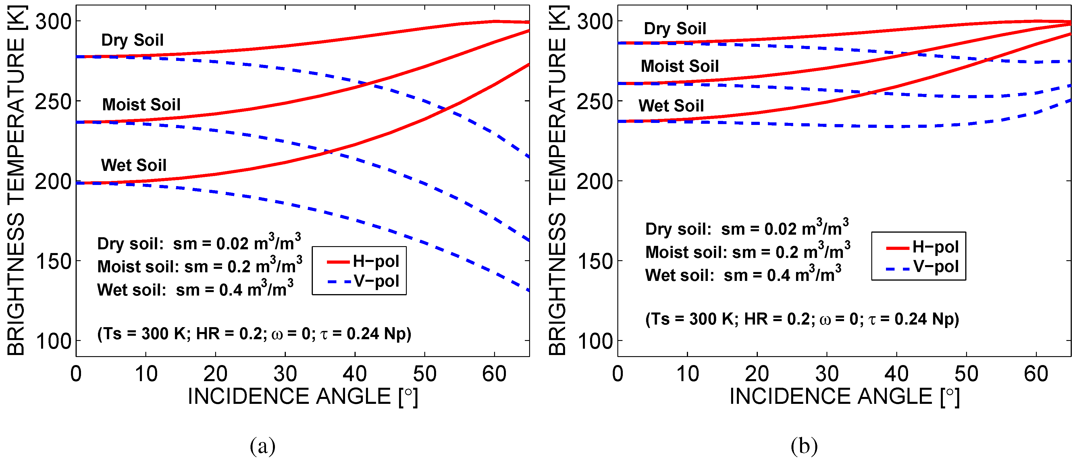
• The effect of the soil moisture content (dry/moist/wet).
• The retrieval formulation using the vertical and horizontal polarizations separately or using the first Stokes parameter.

In Section 2., a description of the scenarios, the forward model and the optimization scheme used in this study to analyze the retrieval of soil moisture from L-band passive observations is provided. A sensitivity analysis of the inversion algorithm is afterwards presented in Section 3. It illustrates the influence that the geophysical variables dominating the Earth’s emission at L-band have on the precision of the retrievals, for the different retrieval configurations. In Section 4., the performance of the different retrieval configurations is analyzed using SMOS-like $T_B$ generated by the SMOS End-to-end Performance Simulator (SEPS) [19]. To obtain soil moisture from SEPS realistic $T_B$, this study uses the L2 Processor Simulator. The L2 Processor Simulator is a dedicated software developed from the experience gained in previous works on SMOS-derived salinity studies [20,21] and land field experiments at L-band [22]; it is a simplified version of the ESA’s SMOS Level 2 Processor, which integrates the forward model and optimization algorithm described on Section 2., and is designed to be used with SEPS output data.

The sensitivity analysis and the analysis with simulated SMOS data are necessary to characterize the different cost function configurations both theoretically and in terms of performance. In Section 5. the main results of this paper are summarized, and their applicability to upcoming SMOS data on an operational basis is discussed.

2. Methodology

2.1. Scenario Definition

In the present study, six master scenarios (bare dry/moist/wet soil and vegetation-covered dry/moist/wet soil) have been defined to evaluate how the soil moisture retrievals can be affected by both the presence of a canopy layer and the soil moisture content itself. These scenarios are homogeneous, described by parameters $s_m$, $T_s$,$HR$,τ and ω, which are constant in all its area; soil moisture values of 0.02 m${}^3$/m${}^3$, 0.2 m${}^3$/m${}^3$, and 0.4 m${}^3$/m${}^3$ have been used for dry, moist and wet soil, respectively, the roughness parameter $HR$ has been set to 0.2, and nominal values are given to the vegetation parameters $\tau =0.24$ Np and $\omega =0$ [23]. A summary of the parameters’ value for each scenario is given in Table 1. Soil texture was assumed to be equal to the mean global clay and sand fractions derived from ECOCLIMAP [24], which are 20.4% and 48.3%, respectively, while soil porosity was assumed to be equal to 38%.

Table 1. Selected original values of soil moisture ($s_m$), soil roughness ($HR$), soil temperature ($T_s$), vegetation albedo (ω) and vegetation opacity (τ) for the six master scenarios. ${\sigma }_{p_i}^0$ is the nominal uncertainty of parameter $p_i$.

		$s_m$ [m${}^3$/m${}^3$]	$HR$	$Ts$ [K]	ω	τ [Np]
		(${\sigma }_{s_m}^0=0.04$)	(${\sigma }_{HR}^0=0.05$)	(${\sigma }_{Ts}^0=2$)	(${\sigma }_{\omega }^0=0.1$)	(${\sigma }_{\tau }^0=0.1$)
Bare	dry soil	0.02	0.2	300	0	0
	moist soil	0.2	0.2	300	0	0
	wet soil	0.4	0.2	300	0	0
Vegetation-covered	dry soil	0.02	0.2	300	0	0.24
	moist soil	0.2	0.2	300	0	0.24
	wet soil	0.4	0.2	300	0	0.24

Table 1. Selected original values of soil moisture ($s_m$), soil roughness ($HR$), soil temperature ($T_s$), vegetation albedo (ω) and vegetation opacity (τ) for the six master scenarios. ${\sigma }_{p_i}^0$ is the nominal uncertainty of parameter $p_i$.

		$s_m$ [m${}^3$/m${}^3$]	$HR$	$Ts$ [K]	ω	τ [Np]
		(${\sigma }_{s_m}^0=0.04$)	(${\sigma }_{HR}^0=0.05$)	(${\sigma }_{Ts}^0=2$)	(${\sigma }_{\omega }^0=0.1$)	(${\sigma }_{\tau }^0=0.1$)
Bare	dry soil	0.02	0.2	300	0	0
	moist soil	0.2	0.2	300	0	0
	wet soil	0.4	0.2	300	0	0
Vegetation-covered	dry soil	0.02	0.2	300	0	0.24
	moist soil	0.2	0.2	300	0	0.24
	wet soil	0.4	0.2	300	0	0.24

2.2. Forward Model

The bare soil emissivity depends on its surface roughness (parameterized using the roughness parameter $HR$), soil temperature $T_s$, and soil dielectric constant, which is in turn related to the soil moisture content $s_m$ and soil type [25]. When the soil is covered by vegetation, its emission is affected by the canopy layer: it attenuates the soil emission and adds its own contribution. The geophysical model function used in this study to mimic the Earth emission at L-band—the so-called forward model—is the well-known $\tau -\omega$ model [26,27]. This model is based on two vegetation parameters, the optical depth or opacity τ, which accounts for the attenuation, and the single scattering albedo ω, which accounts for dispersion of the radiation within the vegetation:

$$T_{pp}=(1-\omega )(1-\gamma )(1+{\Gamma }_S·\gamma )T_V+(1-{\Gamma }_S)T_s·\gamma ,$$

(1)

where $T_{pp}$ ($p=h$ for the horizontal polarization and $p=v$ for the vertical polarization) are the modeled brightness temperatures, ${\Gamma }_S(\theta ,p)$ is the soil reflectivity, $\gamma (\theta ,p)$ is the transmissivity of the vegetation layer, $T_s$ is the effective soil temperature, and $T_V$ the effective temperature of the vegetation.

The soil reflectivity ${\Gamma }_S(\theta ,p)$ depends on incidence angle θ and polarization p, and can be expressed as:

$${\Gamma }_S(\theta ,p)=[(1-Q)·{\Gamma }_S^{*}(\theta ,p)+Q·{\Gamma }_S^{*}(\theta ,p)]·exp(-HR·{cos}^n\left(\theta \right)),$$

(2)

where ${\Gamma }_S^{*}(\theta ,p)$ is the power reflection coefficient of the flat soil (squared amplitude of the Fresnel reflection coefficient) that depends on the soil moisture through the dielectric constant [16], Q is the polarization mixing factor, n expresses the angular dependence of roughness and $HR$ is the soil roughness parameter [28].

The transmissivity of the vegetation layer $\gamma (\theta ,p)$ can be expressed as a function of the vegetation optical thickness τ and the incidence angle θ:

$$\gamma (\theta ,p)=exp(-\tau /cos(\theta \left)\right)$$

(3)

The vegetation optical depth can be linearly related to the vegetation water content, VWC (kg/m${}^2$), through an empirical parameter, b [18]:

$$\tau =b·\mathrm{VWC}$$

(4)

A detailed analysis of the soil roughness effects performed by [29] showed that both Q and n could be set equal to zero at L-band and that the roughness parameter $HR$ could be semi-empirically estimated comprising most surface roughness conditions. This approach has been followed on this study, where $HR$ is set constant and equal to 0.2, representing rather smooth roughness conditions. This is consistent with L-band airborne and ground-based experiments, where soil roughness has generally found to be rather smooth over agricultural or natural areas [30,31]. However, recent experimental studies have estimated values of $HR$ as high as 1 [32,33]; therefore, the effect of having a higher roughness parameter ($HR$ = 1) has been analyzed in Section 4.2. Also, some studies have observed a dependence of HR on soil moisture content [29,34,35]. Nevertheless, this interdependency will not be considered in this work, since these studies have been performed under very local conditions, and yet there is no evidence of the potential benefits that they may introduce at global scale.

There is some experimental evidence indicating possible polarization dependence of both τ and ω. However, this dependence has been observed mainly during field experiments over vegetation that exhibits a predominant orientation, such as vertical stalks in tall grasses, grains and maize [36,37,38], whereas canopy and stem structure of most vegetation covers are randomly oriented. Furthermore, the effects of any systematic orientation of vegetation elements would most likely be minimized at satellite scales [39]. Hence, (1) has been simplified assuming that τ and ω are polarization and angle independent. Also, it is assumed that the temperature of the vegetation canopy is in equilibrium with the soil temperature ($T_s=T_V$), since at SMOS overpass times (6 a.m./6 p.m.) temperature gradients within the soil and vegetation should be minimized [40].

Figure 1 shows the dependence of brightness temperature with incidence angle and polarization for the six scenarios studied, from (1). In the bare soil scenarios on Figure 1(a), it can be seen that H-pol increases with the incidence angle, whereas V-pol decreases with increasing incidence angle. Figure 1 (b) shows that vegetation increases the soil emissivity, and decreases the difference between the vertically and horizontally polarized brightness temperatures, and between the dry and wet soil conditions. This indicates that correction for the effects of vegetation is necessary to obtain accurate soil moisture estimates. Furthermore, retrievals become increasingly unreliable as the opacity of the vegetation layer increases [41]. Figure 1 also illustrates that the emissivity of dry soils is greater than the emissivity of wet soils, with a soil brightness temperature variation at nadir of ∼ 80 K in the bare soil scenarios and of ∼ 40 K in the vegetation-covered scenarios. In the two cases, this variation is much larger than the noise sensitivity threshold of a microwave radiometer (typically < 1 K), so that a large signal-to-noise ratio is obtained. This is a major advantage of the passive microwave technique for soil moisture remote sensing. Likewise, the SMOS mission was defined to make full use of dual-polarized multi-angular L-band acquisitions: by registering a lot of independent information of each pixel, it is expected that soil and vegetation contributions could nicely be separated [9].

Figure 1. Graphical plots illustrating the brightness temperature dependence with incidence angle for (a) the bare soil scenarios, and (b) the vegetation-covered scenarios of Table 1, from (1).

Figure 1. Graphical plots illustrating the brightness temperature dependence with incidence angle for (a) the bare soil scenarios, and (b) the vegetation-covered scenarios of Table 1, from (1).

2.3. Retrieval Algorithm

Soil moisture retrieval consists of inverting the geophysical model function by finding the set of input variables ($s_m$, $T_s$, $HR$, ω and τ) which generate the brightness temperatures that best match the “observed” brightness temperatures. This inversion is performed on the L2 processor by minimizing a cost function which accounts for the weighted squared differences between model and measured data, using the iterative Levenberg-Marquardt method [42].

Assuming that the measurement errors are Gaussian, the fundamental least-squares cost function ($CF$) for observation-model misfits is:

$$CF={({\overline{F}}^{meas}-{\overline{F}}^{model})}^T{C}_F^{-1}({\overline{F}}^{meas}-{\overline{F}}^{model})+{(p_i-p_{i0})}^T{C}_p^{-1}(p_i-p_{i0})$$

(5)

where ${\overline{F}}^{meas}$ and ${\overline{F}}^{model}$ are vectors of length N containing the brightness temperatures at different incidence angles, measured by MIRAS and obtained using the forward models, respectively. N is the number of observations of the same point in a satellite overpass, which ranges from about 240 measurements at the center of the swath to about 20 at 600 km from the sub-satellite track; $C_F$ is the covariance matrix of the brightness temperatures, which depends on the SMOS operation mode and the reference frame [15]; $p_i$ are the retrieved physical parameters that may influence the modeled $T_B$, including $s_m$, $T_s$, $HR$, τ and ω; $p_{i0}$ are prior estimates of parameters $p_i$ (obtained from other sources such as satellite measurements or model outputs, the auxiliary information); and $C_p$ is a diagonal matrix containing the variances of the prior parameters ${\sigma }_{p_{i0}}^2$ [23].

If the model error is uncorrelated between different measurements, then $C_F$ is diagonal, and (5) can be expressed as:

$$CF=\sum _{n=1}^N\frac{\parallel {\overline{F}}_n^{meas}-{\overline{F}}_n^{model}{\parallel }^2}{{\sigma }_{F_n}^2}+\sum _{i=1}^M\frac{{(p_i-p_{i0})}^2}{{\sigma }_{p_{i0}}^2}$$

(6)

where ${\sigma }_{F_n}$ is the radiometric accuracy for the n^th observation, and M is the number of parameters $p_i$ to be retrieved. ${\sigma }_{p_{i0}}$ represents the uncertainty on the a priori parameter $p_{i0}$, and its value is used to parameterize the constraint on the parameter $p_i$ in the retrievals: $p_i$ can be set to be free (${\sigma }_{p_{i0}}=100$, no a priori information is used), it can be constrained to be more or less close to the reference value $p_{i0}$, or it can be constant (${\sigma }_{p_{i0}}<{10}^{-3}$, assuming high accuracy on the a priori information). Note that $p_{i0}$ are specified a priori, whereas $p_i$ values are adjusted during the minimization process.

The retrieval of the geophysical parameters can be formulated using the vertical ($T_{vv}$) and horizontal ($T_{hh}$) polarizations separately (${\overline{F}}_n={[T_{vv},T_{hh}]}^T$ in the Earth reference frame and ${\overline{F}}_n={[T_{xx},T_{yy}]}^T$ in the antenna frame), or using the first Stokes parameter (${\overline{F}}_n={\left[T_I\right]}^T={[T_{xx}+T_{yy}]}^T={[T_{hh}+T_{vv}]}^T$) [6,43]. These two approaches will be considered in this study. Note that, up to date, the formulation of the SMOS-derived soil moisture retrieval problem on the Earth reference frame is the preferred one [14,33]. Hence, we present the formulation of the problem in terms of the first Stokes parameter as an alternative approach, since retrievals using $T_I$ could benefit of having less angular dependency than ($T_{vv},T_{hh}$), therefore reducing the degrees of freedom during the inversion process, which could lead to better soil moisture retrievals. Also, retrievals using $T_I$ are unaffected by geometric and Faraday rotations, which is critical from an operational point of view.

To explore the effect of adding a priori (background) information of other geophysical variables on the minimization process, the two Bayesian-based $CFs$ on Table 2 have been formulated: $C{F}_1$ represents the case in which no a priori information is added, i.e., the cost function consists of an observational term and all parameters are free in the minimization; and $C{F}_2$ stands for the case in which a priori information of all auxiliary parameters is added, excluding $s_m$. Note that, in addition to using or not auxiliary information in the retrievals, it is important to have a good knowledge of the quality of the prior information. Thus, in the present study, $T_s$ is assumed to be known by means of thermal infrared observations and/or meteorological models with an accuracy of 2 K, and the accuracies of $HR$, ω and τ estimations are comprehensively set according to 1) the simulated study in [44], where a large number of retrieval configurations, depending on the a priori information used in the retrievals and its associated uncertainty were tested, and 2) the field experiments in [22].

Table 2. Selected standard deviations of soil moisture ($s_m$), soil roughness ($HR$), soil temperature ($T_s$), vegetation albedo (ω) and vegetation opacity (τ) for the two selected cost function configurations $C{F}_1$ and $C{F}_2$.

	${\sigma }_{s_m}$ [m${}^3$/m${}^3$]	${\sigma }_{HR}$	${\sigma }_{Ts}$ [K]	${\sigma }_{\omega }$	${\sigma }_{\tau }$ [Np]
$C{F}_1$	100	100	100	100	100
$C{F}_2$	100	0.05	2	0.1	0.1

Table 2. Selected standard deviations of soil moisture ($s_m$), soil roughness ($HR$), soil temperature ($T_s$), vegetation albedo (ω) and vegetation opacity (τ) for the two selected cost function configurations $C{F}_1$ and $C{F}_2$.

	${\sigma }_{s_m}$ [m${}^3$/m${}^3$]	${\sigma }_{HR}$	${\sigma }_{Ts}$ [K]	${\sigma }_{\omega }$	${\sigma }_{\tau }$ [Np]
$C{F}_1$	100	100	100	100	100
$C{F}_2$	100	0.05	2	0.1	0.1

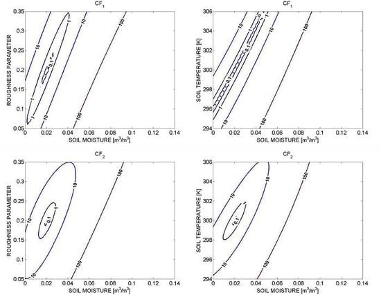
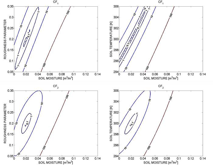
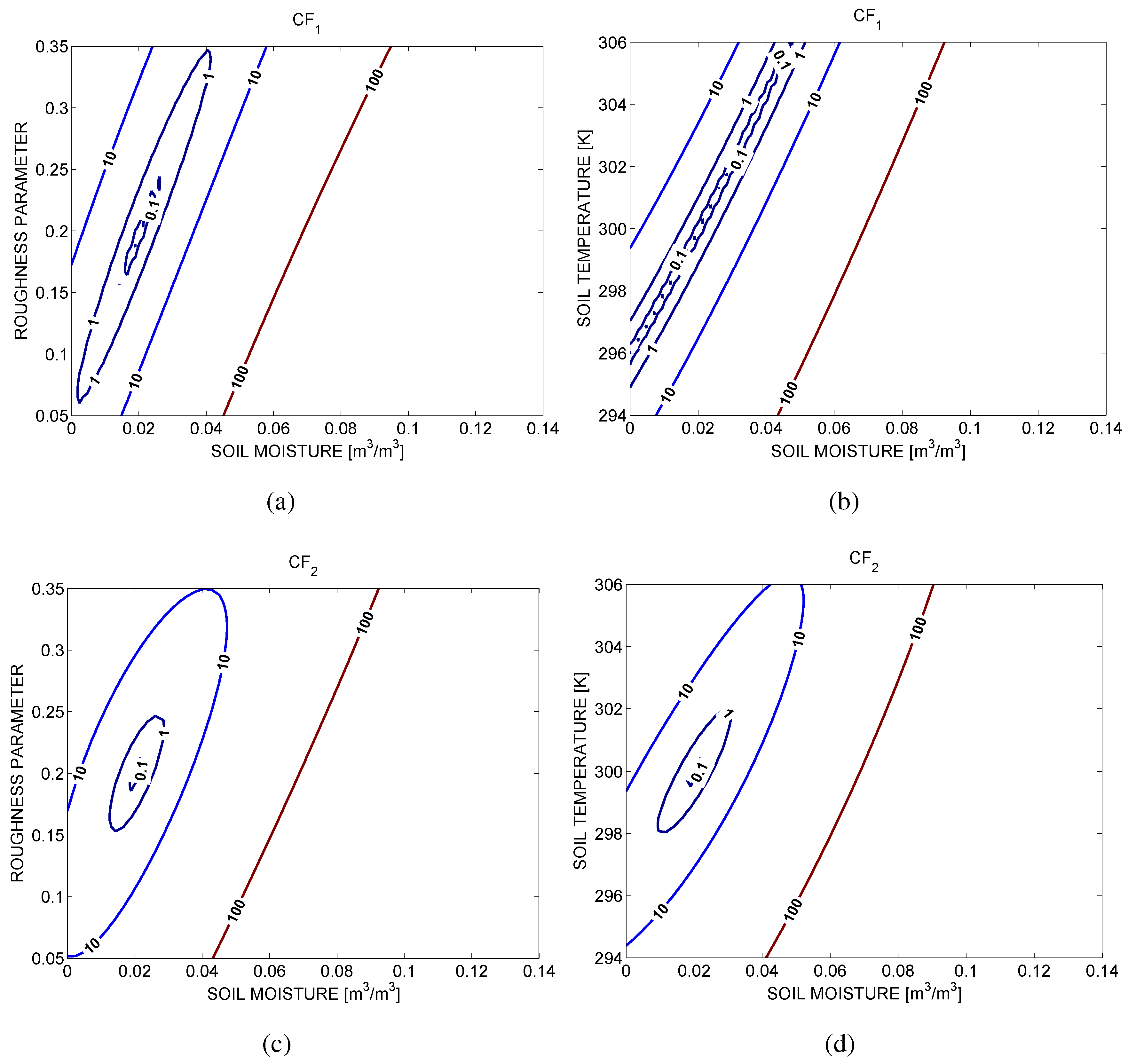
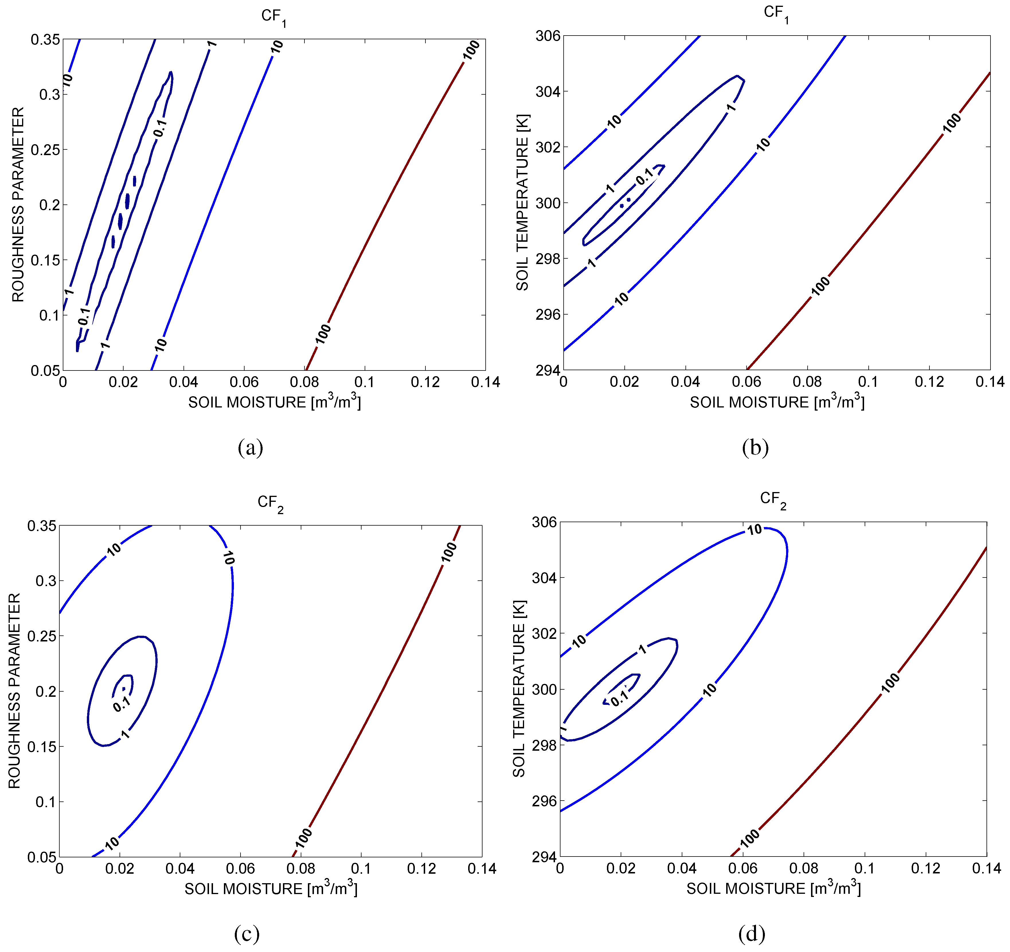
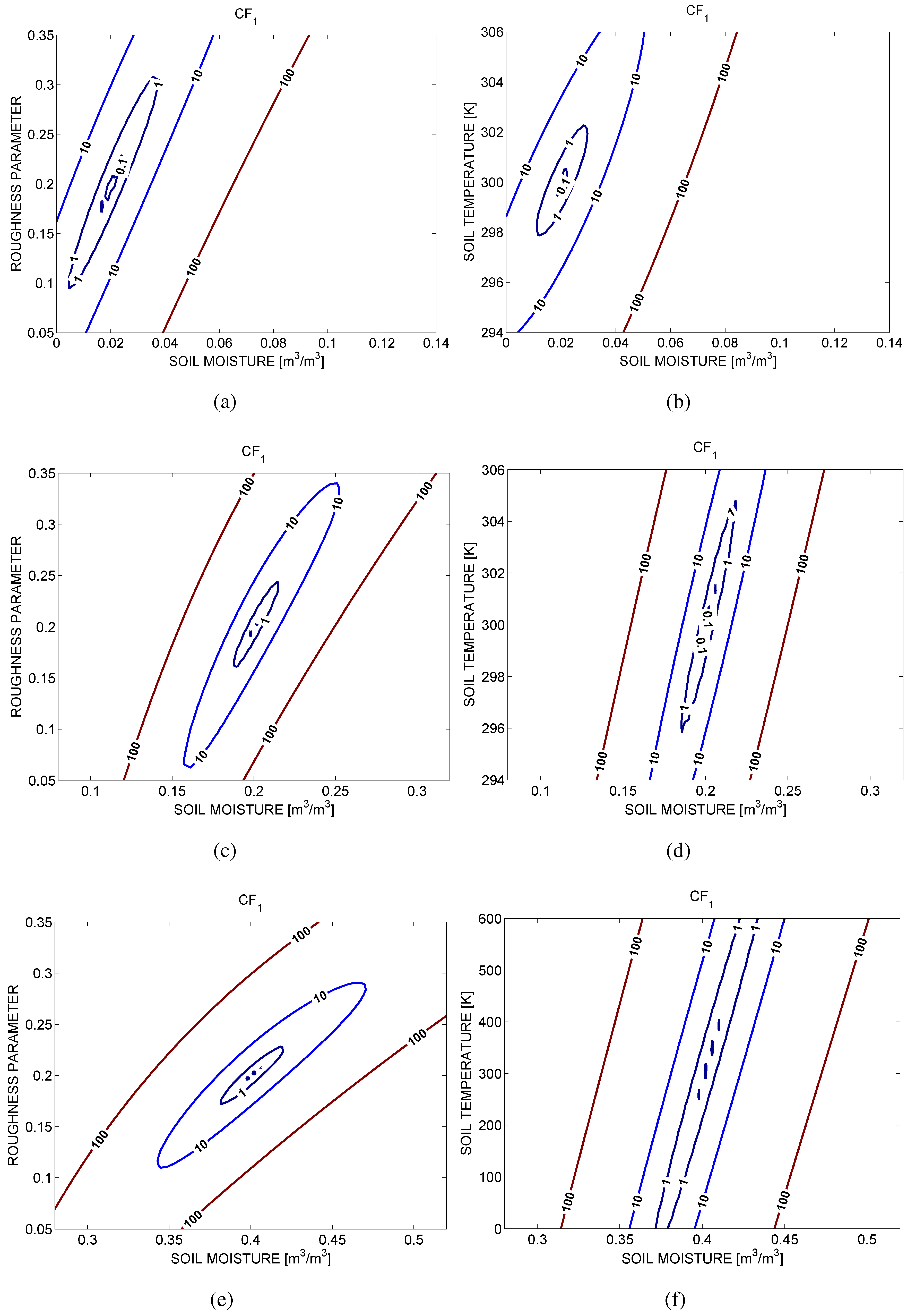
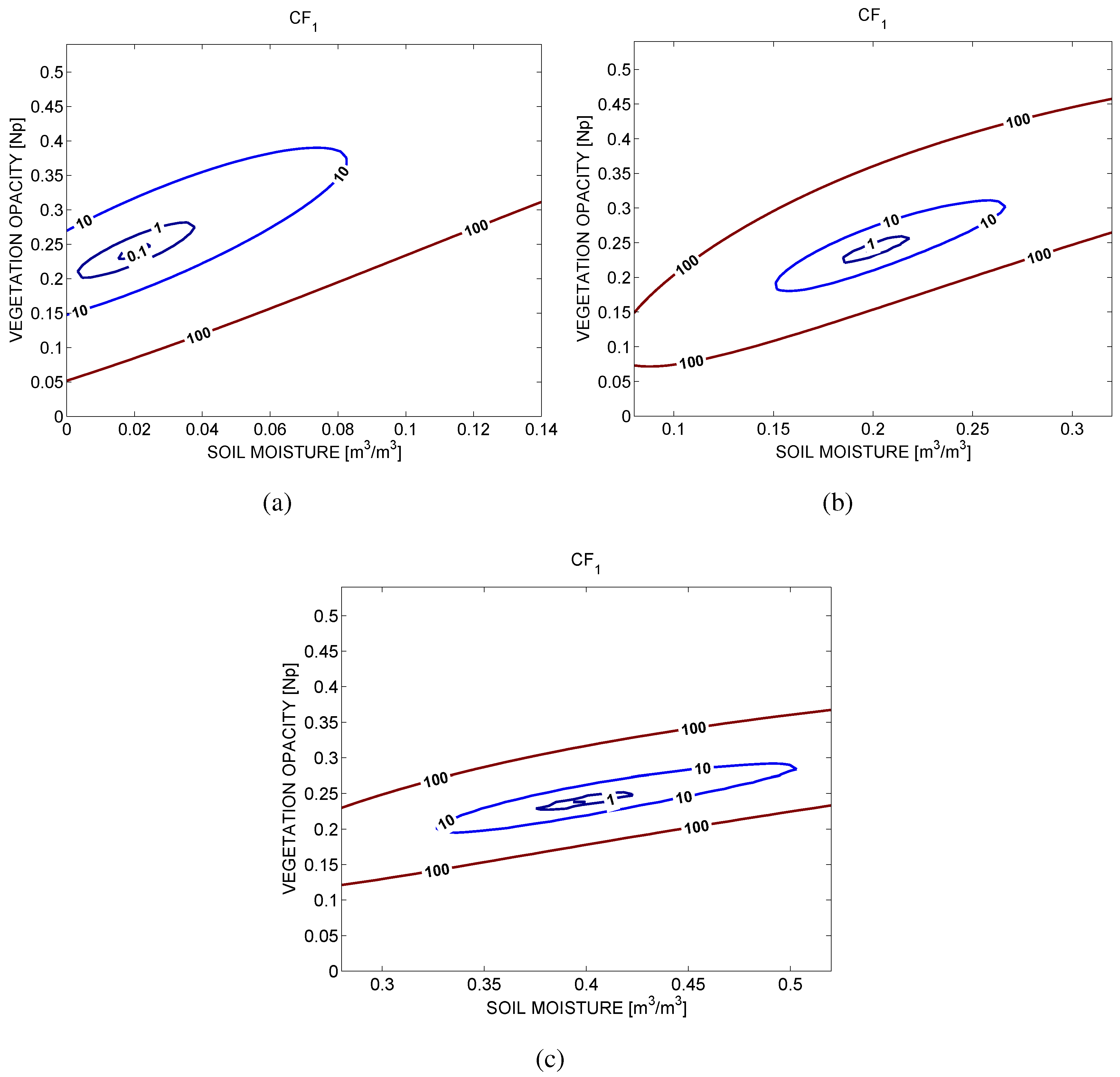
3. Sensitivity Analysis

To get a visual understanding of the $CF$ shape under different configurations, a set of retrieval setups have been formulated from (6), and the most interesting sections (2-D contours) are visualized showing the behavior of the minima in 2-D cuts through a 5-D $CF$, where the 5-D are the parameters of the forward model, namely $s_m$, $T_s$, $HR$, ω and τ. These contour plots indicate in the first place that the $CF$ has only one minimum and converges to the original values, as expected. Note that this is important to ensure that the minimization algorithm will be approaching the “true” solution, and not a local minimum. Also, the $CF$ can be interpreted as the misfit of the measurements with the solution lying on the geophysical model function surface. Therefore, the shape of its minimum determines the precision of the retrieval. The broader the minimum, the less accurate are the retrieved parameters, since we are ignoring all the neighboring solutions, which have a comparable probability of being the true state (as represented by the original $s_m$, $HR$, $T_s$, ω and τ on Table 1) [45,46].

The weights of (6) were set according to Table 2, with ${\sigma }_{T_B}=2$ K. The original parameters (“measured”) were set according to the scenario simulated (see the parameters’ original values for each scenario on Table 1) and the forward model on Section 2.2. was used to simulate $T{B}^{meas}$ for incidence angles between 0${}^{\circ }$ and 65${}^{\circ }$. Likewise, this was done to obtain $T{B}^{model}$ over the ranges $0\le s_m\le 0.5$ m${}^3$/m${}^3$, $250\le T_s\le 350$ K, $0\le HR\le 5$, $0\le \tau \le 3$ Np, and $0\le \omega \le 0.3$ [23]. Hence, when the scenario’s original values are used $T{B}^{model}$ equals $T{B}^{meas}$, which corresponds to the $CF$’s absolute minimum. Note that the axis on the figures have been normalized to the parameters’ original values $\pm 3·{\sigma }_{p_i}^0$ to cover the 99.7% of the values the retrieved parameters could have and properly compare the different contours. Since the purpose of this experiment is to evaluate the sensitivities (gradients) of the different cost function configurations, no bias errors are assumed in measurements or references; the effect of having an a priori value which is far from the true state is analyzed in Section 4.

Figure 2 shows $CFs$ formulated using the first Stokes parameter over a bare dry soil scenario for the case where no constraints are added (Figure 2 (a) and (b)) and for the case where a priori information about all the auxiliary parameters, except for $s_m$, is added (Figure 2 (c) and (d)). It can be seen that the minimum in the case of no constraints is elliptical with its major axis covering almost the entire range of roughness parameter and soil temperature values for the contour line $CF=1$. This indicates a low sensitivity to $HR$ and $T_s$ and a high sensitivity to $s_m$. When the constraints are used the minimum is better defined, i.e., there is a higher probability of finding the true state. This effect is also manifested on vegetation-covered simulations (see Figure 3). Therefore, assuming that both the real errors in $T_B$ and the reference values are Gaussian, a constrained $CF$ should lead to a more accurate $s_m$ retrieval than a non-constrained $CF$.

Figure 2. Cost functions formulated using $T_I$ over a bare dry soil scenario. Contours of $HR$ vs $s_m$ (a) and $T_s$ vs $s_m$ (b), with no constraints on the cost function ($C{F}_1$). Contours of $HR$ vs $s_m$ (c) and $T_s$ vs $s_m$ (d), adding constraints on all parameters, except for $s_m$ ($C{F}_2$).

Figure 2. Cost functions formulated using $T_I$ over a bare dry soil scenario. Contours of $HR$ vs $s_m$ (a) and $T_s$ vs $s_m$ (b), with no constraints on the cost function ($C{F}_1$). Contours of $HR$ vs $s_m$ (c) and $T_s$ vs $s_m$ (d), adding constraints on all parameters, except for $s_m$ ($C{F}_2$).

The presence of a sparse vegetation layer is examined in Figure 3. It can be noticed that the contours plotted are clearly widened if compared to those on Figure 2, which indicates a higher uncertainty in the soil moisture retrievals over vegetation-covered surfaces, as expected. The vegetation canopy attenuates the soil emission and diminishes the forward model sensitivity to $s_m$; as the observed soil emissivity decreases with an increase in vegetation biomass, the soil moisture information contained in the microwave signal decreases [6].

Figure 3. Cost functions formulated using $T_I$ over a vegetation-covered dry soil scenario. Contours of $HR$ vs. $s_m$ (a) and $T_s$ vs $s_m$ (b), with no constraints on the cost function ($C{F}_1$). Contours of $HR$ vs $s_m$ (c) and $T_s$ vs $s_m$ (d), adding constraints on all parameters, except for $s_m$ ($C{F}_2$).

Figure 3. Cost functions formulated using $T_I$ over a vegetation-covered dry soil scenario. Contours of $HR$ vs. $s_m$ (a) and $T_s$ vs $s_m$ (b), with no constraints on the cost function ($C{F}_1$). Contours of $HR$ vs $s_m$ (c) and $T_s$ vs $s_m$ (d), adding constraints on all parameters, except for $s_m$ ($C{F}_2$).

The difference between $CFs$ simulated over a bare dry, moist, and wet soil scenario can be seen in Figure 4. The cost function sensitivity to $HR$ is the highest on wet soils (Figure 4 (e)) and the lowest on dry soils (Figure 4 (a)). In contrast, the cost function sensitivity to $T_s$ is the highest on dry soils (Figure 4 (b)) and the lowest on wet soils (Figure 4 (f)). Therefore, constraints on both $HR$ and $T_s$ should be needed to improve the accuracy of soil moisture retrievals over bare soils under diverse moist conditions. This result can also be extended to vegetation-covered scenarios, where the same behavior has been observed in the $CFs$. Note that the plots on Figure 2 and Figure 4 are in good agreement with other L-band retrieval studies [14,47], where adding constraints on $HR$ and $T_s$ was also shown to be preferable.

Figure 4. Cost functions formulated using $T_{hh}-T_{vv}$ with no constraints. Contours of $HR$ vs. $s_m$ (a) and $T_s$ vs $s_m$ (b) over a bare dry soil scenario. Contours of $HR$ vs. $s_m$ (c) and $T_s$ vs $s_m$ (d) over a bare moist soil scenario. Contours of $HR$ vs. $s_m$ (e) and $T_s$ vs $s_m$ (f) over a bare wet soil scenario.

Figure 4. Cost functions formulated using $T_{hh}-T_{vv}$ with no constraints. Contours of $HR$ vs. $s_m$ (a) and $T_s$ vs $s_m$ (b) over a bare dry soil scenario. Contours of $HR$ vs. $s_m$ (c) and $T_s$ vs $s_m$ (d) over a bare moist soil scenario. Contours of $HR$ vs. $s_m$ (e) and $T_s$ vs $s_m$ (f) over a bare wet soil scenario.

Regarding the vegetation parameters, Figure 5 shows that the $CF$ sensitivity to τ is the highest over vegetation-covered wet soils and decreases as the soil under the vegetation canopy dries out, as can be easily appreciated in the contour line $CF=10$. This indicates that better τ retrievals should be expected over wet than over dry soils. The effect of adding restrictions on τ and ω in the $CF$ was not clearly visible in the contours, probably because the restrictions imposed on these variables are not very severe (${\sigma }_{\tau }={\sigma }_{\omega }=0.1$). However, it is shown to actually improve $s_m$ and τ retrievals when applied to SMOS-like simulated data on Section 4.2.

Figure 5. Cost functions formulated using $T_{hh}-T_{vv}$ with no constraints. Contours of τ vs. $s_m$ (a) over a vegetation-covered dry scenario. Contours of τ vs. $s_m$ (b) over a vegetation-covered moist scenario. Contours of τ vs. $s_m$ (c) over a vegetation-covered wet scenario.

Figure 5. Cost functions formulated using $T_{hh}-T_{vv}$ with no constraints. Contours of τ vs. $s_m$ (a) over a vegetation-covered dry scenario. Contours of τ vs. $s_m$ (b) over a vegetation-covered moist scenario. Contours of τ vs. $s_m$ (c) over a vegetation-covered wet scenario.

Comparing Figure 3(a) and (b) with Figure 4(a) and (b), it can be observed that the $CF$ sensitivity to $T_s$ is higher when using the $T_{hh}-T_{vv}$ than when using $T_I$, whereas the sensitivity to $HR$ remains the same. No remarkable differences have been found between the two formulations over vegetation-covered scenarios.

4. Analysis with Simulated SMOS Data

4.1. Simulation Strategy

L-band 2-D multi-angular brightness temperatures over land have been simulated for the six main surface conditions of Table 1 using SEPS. Next, these data has been used as input to the L2 Processor Simulator, where retrievals have been performed using the three $CF$ configurations of Table 2, formulated in terms of vertical ($T_{vv}$) and horizontal ($T_{hh}$) polarizations separately and using the first Stokes parameter ($T_I$). Note that over the bare soil scenarios $\tau =\omega =0$ will not be retrieved. It is important to outline that SEPS simulated error on $T_B$ includes all the instrument specific features (measured antenna pattern, measured receivers’ frequency response, thermal drifts, etc.) and all the realistic features induced by the image reconstruction algorithms, such as biases and the pixel-dependent radiometric accuracy [48].

Retrievals on the L2 Processor Simulator have been performed under the following guidelines and assumptions:

–

The geophysical models and the ancillary data used in the L2 Processor Simulator are the same as in SEPS, so that the effect of the model used is not affecting the results.

–

The performance of the $CF$ configuration is not dependent on ${\sigma }_{F_n}$, since the absolute accuracy of the radiometric measurements is available on the SEPS output and is used in L2 Processor Simulator.

–

To reduce the computational time, the search limits of the retrieved variables in the $CF$ have been reduced within reasonable bounds, namely $0\le s_m\le 0.5$ m${}^3$/m${}^3$, $250\le T_s\le 350$ K, $0\le HR\le 5$, $0\le \tau \le 3$ Np, and $0\le \omega \le 0.3$ [23].

–

The reference values of the parameters on the $CF$ ($p_{i0}$) are randomly determined from a normal distribution with the nominal standard deviations on Table 1, added to the original values.

–

Homogeneous pixels have been assumed in the simulations to evidence the contribution of each parameter in the results and facilitate the analysis. However, further studies will be required to assess the limitations imposed by heterogeneity of vegetation cover and soil characteristics within a satellite footprint.

4.2. Simulation Results

The mean, standard deviation, and RMSE of the retrieved soil moisture $(s_m^{ret}-s_m^{orig})$ are shown in Table 3 for the bare soil scenarios and in Table 4 for the vegetation-covered scenarios defined in Table 1. It can be seen that in the case of no constraints ($C{F}_1$), the SMOS $s_m$ science requirement of 0.04 m${}^3$/m${}^3$ is not met for any of the scenarios simulated: a retrieval error of ≈ 0.10 to 0.21 m${}^3$/m${}^3$ is obtained over bare soils and of ≈ 0.11 to 0.24 m${}^3$/m${}^3$ over vegetation-covered soils.

Table 3. Retrieved mean, standard deviation and root mean square soil moisture error of simulated SMOS observations over the bare soil scenarios on Table 1, using the cost function configurations of Table 2, formulated on the Earth reference frame or using the first Stokes parameter.

Scenario	Retrieved $s_m$ error	$C{F}_1$ ($\raisebox{1ex}{$HR=0.2$}\!\left/ \!\raisebox{-1ex}{$HR=1$}\right.$)		$C{F}_2$ ($\raisebox{1ex}{$HR=0.2$}\!\left/ \!\raisebox{-1ex}{$HR=1$}\right.$)
		Earth	Stokes	Earth	Stokes
Bare Dry Soil	Mean	$\raisebox{1ex}{$0.149$}\!\left/ \!\raisebox{-1ex}{$0.185$}\right.$	$\raisebox{1ex}{$0.106$}\!\left/ \!\raisebox{-1ex}{$0.140$}\right.$	$\raisebox{1ex}{$0.026$}\!\left/ \!\raisebox{-1ex}{$0.038$}\right.$	$\raisebox{1ex}{$0.010$}\!\left/ \!\raisebox{-1ex}{$0.021$}\right.$
	Std. dev.	$\raisebox{1ex}{$0.157$}\!\left/ \!\raisebox{-1ex}{$0.179$}\right.$	$\raisebox{1ex}{$0.164$}\!\left/ \!\raisebox{-1ex}{$0.160$}\right.$	$\raisebox{1ex}{$0.092$}\!\left/ \!\raisebox{-1ex}{$0.102$}\right.$	$\raisebox{1ex}{$0.024$}\!\left/ \!\raisebox{-1ex}{$0.039$}\right.$
	RMS	$\raisebox{1ex}{$0.216$}\!\left/ \!\raisebox{-1ex}{$0.257$}\right.$	$\raisebox{1ex}{$0.196$}\!\left/ \!\raisebox{-1ex}{$0.211$}\right.$	$\raisebox{1ex}{$0.096$}\!\left/ \!\raisebox{-1ex}{$0.108$}\right.$	$\raisebox{1ex}{$0.027$}\!\left/ \!\raisebox{-1ex}{$0.044$}\right.$
Bare Moist Soil	Mean	$\raisebox{1ex}{$0.069$}\!\left/ \!\raisebox{-1ex}{$0.059$}\right.$	$\raisebox{1ex}{$0.018$}\!\left/ \!\raisebox{-1ex}{$0.056$}\right.$	$\raisebox{1ex}{$-0.014$}\!\left/ \!\raisebox{-1ex}{$-0.050$}\right.$	$\raisebox{1ex}{$-0.006$}\!\left/ \!\raisebox{-1ex}{$0.006$}\right.$
	Std. dev.	$\raisebox{1ex}{$0.122$}\!\left/ \!\raisebox{-1ex}{$0.160$}\right.$	$\raisebox{1ex}{$0.134$}\!\left/ \!\raisebox{-1ex}{$0.143$}\right.$	$\raisebox{1ex}{$0.085$}\!\left/ \!\raisebox{-1ex}{$0.105$}\right.$	$\raisebox{1ex}{$0.039$}\!\left/ \!\raisebox{-1ex}{$0.054$}\right.$
	RMS	$\raisebox{1ex}{$0.140$}\!\left/ \!\raisebox{-1ex}{$0.171$}\right.$	$\raisebox{1ex}{$0.135$}\!\left/ \!\raisebox{-1ex}{$0.154$}\right.$	$\raisebox{1ex}{$0.085$}\!\left/ \!\raisebox{-1ex}{$0.116$}\right.$	$\raisebox{1ex}{$0.039$}\!\left/ \!\raisebox{-1ex}{$0.054$}\right.$
Bare Wet Soil	Mean	$\raisebox{1ex}{$-0.056$}\!\left/ \!\raisebox{-1ex}{$-0.100$}\right.$	$\raisebox{1ex}{$-0.081$}\!\left/ \!\raisebox{-1ex}{$-0.090$}\right.$	$\raisebox{1ex}{$-0.052$}\!\left/ \!\raisebox{-1ex}{$-0.113$}\right.$	$\raisebox{1ex}{$-0.038$}\!\left/ \!\raisebox{-1ex}{$-0.031$}\right.$
	Std. dev.	$\raisebox{1ex}{$0.084$}\!\left/ \!\raisebox{-1ex}{$0.142$}\right.$	$\raisebox{1ex}{$0.096$}\!\left/ \!\raisebox{-1ex}{$0.130$}\right.$	$\raisebox{1ex}{$0.050$}\!\left/ \!\raisebox{-1ex}{$0.088$}\right.$	$\raisebox{1ex}{$0.032$}\!\left/ \!\raisebox{-1ex}{$0.037$}\right.$
	RMS	$\raisebox{1ex}{$0.101$}\!\left/ \!\raisebox{-1ex}{$0.173$}\right.$	$\raisebox{1ex}{$0.125$}\!\left/ \!\raisebox{-1ex}{$0.158$}\right.$	$\raisebox{1ex}{$0.072$}\!\left/ \!\raisebox{-1ex}{$0.143$}\right.$	$\raisebox{1ex}{$0.050$}\!\left/ \!\raisebox{-1ex}{$0.048$}\right.$

Table 3. Retrieved mean, standard deviation and root mean square soil moisture error of simulated SMOS observations over the bare soil scenarios on Table 1, using the cost function configurations of Table 2, formulated on the Earth reference frame or using the first Stokes parameter.

Scenario	Retrieved $s_m$ error	$C{F}_1$ ($\raisebox{1ex}{$HR=0.2$}\!\left/ \!\raisebox{-1ex}{$HR=1$}\right.$)		$C{F}_2$ ($\raisebox{1ex}{$HR=0.2$}\!\left/ \!\raisebox{-1ex}{$HR=1$}\right.$)
		Earth	Stokes	Earth	Stokes
Bare Dry Soil	Mean	$\raisebox{1ex}{$0.149$}\!\left/ \!\raisebox{-1ex}{$0.185$}\right.$	$\raisebox{1ex}{$0.106$}\!\left/ \!\raisebox{-1ex}{$0.140$}\right.$	$\raisebox{1ex}{$0.026$}\!\left/ \!\raisebox{-1ex}{$0.038$}\right.$	$\raisebox{1ex}{$0.010$}\!\left/ \!\raisebox{-1ex}{$0.021$}\right.$
	Std. dev.	$\raisebox{1ex}{$0.157$}\!\left/ \!\raisebox{-1ex}{$0.179$}\right.$	$\raisebox{1ex}{$0.164$}\!\left/ \!\raisebox{-1ex}{$0.160$}\right.$	$\raisebox{1ex}{$0.092$}\!\left/ \!\raisebox{-1ex}{$0.102$}\right.$	$\raisebox{1ex}{$0.024$}\!\left/ \!\raisebox{-1ex}{$0.039$}\right.$
	RMS	$\raisebox{1ex}{$0.216$}\!\left/ \!\raisebox{-1ex}{$0.257$}\right.$	$\raisebox{1ex}{$0.196$}\!\left/ \!\raisebox{-1ex}{$0.211$}\right.$	$\raisebox{1ex}{$0.096$}\!\left/ \!\raisebox{-1ex}{$0.108$}\right.$	$\raisebox{1ex}{$0.027$}\!\left/ \!\raisebox{-1ex}{$0.044$}\right.$
Bare Moist Soil	Mean	$\raisebox{1ex}{$0.069$}\!\left/ \!\raisebox{-1ex}{$0.059$}\right.$	$\raisebox{1ex}{$0.018$}\!\left/ \!\raisebox{-1ex}{$0.056$}\right.$	$\raisebox{1ex}{$-0.014$}\!\left/ \!\raisebox{-1ex}{$-0.050$}\right.$	$\raisebox{1ex}{$-0.006$}\!\left/ \!\raisebox{-1ex}{$0.006$}\right.$
	Std. dev.	$\raisebox{1ex}{$0.122$}\!\left/ \!\raisebox{-1ex}{$0.160$}\right.$	$\raisebox{1ex}{$0.134$}\!\left/ \!\raisebox{-1ex}{$0.143$}\right.$	$\raisebox{1ex}{$0.085$}\!\left/ \!\raisebox{-1ex}{$0.105$}\right.$	$\raisebox{1ex}{$0.039$}\!\left/ \!\raisebox{-1ex}{$0.054$}\right.$
	RMS	$\raisebox{1ex}{$0.140$}\!\left/ \!\raisebox{-1ex}{$0.171$}\right.$	$\raisebox{1ex}{$0.135$}\!\left/ \!\raisebox{-1ex}{$0.154$}\right.$	$\raisebox{1ex}{$0.085$}\!\left/ \!\raisebox{-1ex}{$0.116$}\right.$	$\raisebox{1ex}{$0.039$}\!\left/ \!\raisebox{-1ex}{$0.054$}\right.$
Bare Wet Soil	Mean	$\raisebox{1ex}{$-0.056$}\!\left/ \!\raisebox{-1ex}{$-0.100$}\right.$	$\raisebox{1ex}{$-0.081$}\!\left/ \!\raisebox{-1ex}{$-0.090$}\right.$	$\raisebox{1ex}{$-0.052$}\!\left/ \!\raisebox{-1ex}{$-0.113$}\right.$	$\raisebox{1ex}{$-0.038$}\!\left/ \!\raisebox{-1ex}{$-0.031$}\right.$
	Std. dev.	$\raisebox{1ex}{$0.084$}\!\left/ \!\raisebox{-1ex}{$0.142$}\right.$	$\raisebox{1ex}{$0.096$}\!\left/ \!\raisebox{-1ex}{$0.130$}\right.$	$\raisebox{1ex}{$0.050$}\!\left/ \!\raisebox{-1ex}{$0.088$}\right.$	$\raisebox{1ex}{$0.032$}\!\left/ \!\raisebox{-1ex}{$0.037$}\right.$
	RMS	$\raisebox{1ex}{$0.101$}\!\left/ \!\raisebox{-1ex}{$0.173$}\right.$	$\raisebox{1ex}{$0.125$}\!\left/ \!\raisebox{-1ex}{$0.158$}\right.$	$\raisebox{1ex}{$0.072$}\!\left/ \!\raisebox{-1ex}{$0.143$}\right.$	$\raisebox{1ex}{$0.050$}\!\left/ \!\raisebox{-1ex}{$0.048$}\right.$

Table 4. Retrieved mean, standard deviation and root mean square soil moisture error of simulated SMOS observations over the vegetation-covered scenarios on Table 1, using the cost function configurations of Table 2, formulated on the Earth reference frame or using the first Stokes parameter.

Scenario	Retrieved $s_m$ error	$C{F}_1$		$C{F}_2$
		Earth	Stokes	Earth	Stokes
Dry Soil + Canopy	Mean	0.169	0.170	0.060	0.049
	Std. dev.	0.162	0.169	0.116	0.053
	RMS	0.235	0.240	0.131	0.072
Moist Soil + Canopy	Mean	0.076	0.095	0.003	0.048
	Std. dev.	0.143	0.121	0.120	0.076
	RMS	0.162	0.153	0.120	0.090
Wet Soil + Canopy	Mean	-0.062	-0.040	-0.061	-0.021
	Std. dev.	0.119	0.102	0.093	0.050
	RMS	0.134	0.109	0.111	0.054

Table 4. Retrieved mean, standard deviation and root mean square soil moisture error of simulated SMOS observations over the vegetation-covered scenarios on Table 1, using the cost function configurations of Table 2, formulated on the Earth reference frame or using the first Stokes parameter.

Scenario	Retrieved $s_m$ error	$C{F}_1$		$C{F}_2$
		Earth	Stokes	Earth	Stokes
Dry Soil + Canopy	Mean	0.169	0.170	0.060	0.049
	Std. dev.	0.162	0.169	0.116	0.053
	RMS	0.235	0.240	0.131	0.072
Moist Soil + Canopy	Mean	0.076	0.095	0.003	0.048
	Std. dev.	0.143	0.121	0.120	0.076
	RMS	0.162	0.153	0.120	0.090
Wet Soil + Canopy	Mean	-0.062	-0.040	-0.061	-0.021
	Std. dev.	0.119	0.102	0.093	0.050
	RMS	0.134	0.109	0.111	0.054

Table 3 shows that the $s_m$ retrieval error over bare soil scenarios is considerably improved when constraints on $HR$ and $T_s$ are used ($C{F}_2$): $s_m$ RMSE retrievals of ≈ 0.07 to 0.09 m${}^3$/m${}^3$ are obtained using $T_{hh}-T_{vv}$ and of ≈ 0.03 to 0.05 m${}^3$/m${}^3$ using $T_I$. This result is in line with Figure 2 and with other L-band retrieval studies [14,47]. The special case with $HR$ = 1 on the bare soil scenarios has also been simulated. Results show that a higher roughness leads to an increased $s_m$ RMSE in all the scenarios and configurations studied, and only in the case of using $T_I$ and $C{F}_2$ the $s_m$ retrieval error is below 0.05 m${}^3$/m${}^3$. Table 4 shows that the $s_m$ retrieval error over vegetation-covered scenarios (τ = 0.24 Np and ω = 0) is also improved when constraints on $HR$, $T_s$, ω, and τ are used ($C{F}_2$): $s_m$ RMSE retrievals of ≈ 0.11 to 0.13 m${}^3$/m${}^3$ are obtained using $T_{hh}-T_{vv}$ and of ≈ 0.05 to 0.09 m${}^3$/m${}^3$ using $T_I$. This result is in agreement with Figure 3. Hence, simulation results show that that the use of adequate constraints on the $CF$ improve the accuracy of $s_m$ retrievals in all the cases studied, and that the formulation in terms of $T_I$ is advantageous. Note that the improvement in $s_m$ retrievals when using $C{F}_2$ is specially noticeable in all the scenarios under dry soil conditions, where a remarkably high $s_m$ RMSE is obtained using $C{F}_1$. In fact, lower $s_m$ RMSE is obtained over wet soils than over dry soils (bare and vegetation-covered), except for the case of bare soil retrievals using $T_I$ and $C{F}_2$. This could be due to the reduced sensitivity of the dielectric constant at low moisture levels [49].

Table 5. Retrieved mean, standard deviation and root mean square vegetation opacity error of simulated SMOS observations over the vegetation-covered scenarios on Table 1, using the cost function configurations of Table 2, formulated on the Earth reference frame or using the first Stokes parameter.

Scenario	Retrieved τ error	$C{F}_1$		$C{F}_2$
		Earth	Stokes	Earth	Stokes
Dry Soil + Canopy	Mean	0.439	0.369	0.110	0.036
	Std. dev.	0.888	0.606	0.307	0.085
	RMS	0.991	0.709	0.326	0.092
Moist Soil + Canopy	Mean	0.224	0.100	0.049	0.025
	Std. dev.	0.732	0.342	0.267	0.078
	RMS	0.765	0.356	0.272	0.082
Wet Soil + Canopy	Mean	0.187	0.019	0.053	-0.029
	Std. dev.	0.714	0.208	0.274	0.056
	RMS	0.738	0.209	0.279	0.063

Table 5. Retrieved mean, standard deviation and root mean square vegetation opacity error of simulated SMOS observations over the vegetation-covered scenarios on Table 1, using the cost function configurations of Table 2, formulated on the Earth reference frame or using the first Stokes parameter.

Scenario	Retrieved τ error	$C{F}_1$		$C{F}_2$
		Earth	Stokes	Earth	Stokes
Dry Soil + Canopy	Mean	0.439	0.369	0.110	0.036
	Std. dev.	0.888	0.606	0.307	0.085
	RMS	0.991	0.709	0.326	0.092
Moist Soil + Canopy	Mean	0.224	0.100	0.049	0.025
	Std. dev.	0.732	0.342	0.267	0.078
	RMS	0.765	0.356	0.272	0.082
Wet Soil + Canopy	Mean	0.187	0.019	0.053	-0.029
	Std. dev.	0.714	0.208	0.274	0.056
	RMS	0.738	0.209	0.279	0.063

Vegetation opacity retrievals are analyzed on Table 5. It shows that a notable improvement on τ RMSE is obtained when adequate constraints on the $CF$ are used ($C{F}_2$) than when all parameters are free ($C{F}_1$). Also, results indicate that better τ retrievals should be obtained over wet soils than over dry soils, in agreement with Figure 5. It can be also be seen that better τ retrievals are obtained using $T_I$ than using $T_{hh}-T_{vv}$ in all scenarios and configurations, specially under moist and wet soil conditions. From (4), the optical depth can be linearly related to the VWC using the so-called b parameter, which depends mainly of crop type and frequency. At L-band, $b=0.15$ m${}^2$/kg was found to be representative of most agricultural crops, with the exception of grasses [18]. This value has been used in this study to evaluate if VWC maps with an accuracy of $0.2$ kg/m${}^2$ could be obtained from the τ retrievals on Table 5. Thus, using this approach and considering that no constraints are added, VWC with an accuracy of ≈ 4.9 to 6.6 kg/m${}^2$ could be obtained using $T_{hh}-T_{vv}$ and of ≈ 1.4 to 4.7 kg/m${}^2$ using $T_I$. If constraints are added, the accuracy of VWC improves to ≈ 1.9 to 2.2 kg/m${}^2$ using $T_{hh}-T_{vv}$ and to ≈ 0.4 to 0.6 kg/m${}^2$ using $T_I$. These results show that the formulation in terms of $T_I$ and the use of constraints on the $CF$ substantially improve τ retrievals, although the VWC requirement of 0.2 kg/m${}^2$ is not fully satisfied.

It must be remarked that in the results presented on Table 3, Table 4, and Table 5, all pixels in the SMOS field-of-view (FOV) are considered, regardless of the number of measurements on each pixel. However, due to the SMOS observation geometry, all pixels in the FOV do not have the same properties: as the pixel’s distance to the ground-track increases, the pixel is imaged fewer times, its angular variation is reduced and the instrument’s noise increases [15]. This fact indicates that better accuracies should be expected if only the central part of the FOV—the so-called Narrow Swath (640-km) [50]—is considered. However, note that the use of Narrow Swath implicates a temporal resolution of 7 days, which will limit the applicability of the data. Still, the possibility of increasing the accuracy of the retrievals by considering a narrower swath should not be neglected. Hence, the retrieval performance has been explored further in Figure 6 and Figure 7, as a function of the ground-track distance.

Figure 6 illustrates the soil moisture retrieval performance vs. the pixel position, for all the retrieval configurations and scenarios studied. On the left-hand side of each plot simulation results correspond to the use of the first Stokes parameter, and on the right-hand side to the use of the Earth reference frame. Figure 6 (a) and (b) show results over bare soil scenarios using $C{F}_1$ and $C{F}_2$, respectively. Figure 6 (c) and (d) show results over vegetation-covered scenarios using $C{F}_1$ and $C{F}_2$, respectively. Vertical lines denote the Narrow Swath. These plots effectively show how the $s_m$ RMSE increases with the distance to the ground-track. Also, it can be seen that the use of adequate constraints ($C{F}_2$) dramatically improves soil moisture retrievals. Note that either in the case of considering the nominal or the Narrow Swath, the use of $C{F}_2$ and formulation in terms of $T_I$ should provide more accurate soil moisture retrievals.

Likewise, Figure 7 illustrates the vegetation opacity retrieval performance vs. the pixel position, for all the retrieval configurations and scenarios studied. When no constraints are added (Figure 7 (a)), the retrieval error rapidly increases beyond the Narrow Swath width. If adequate constraints are added (Figure 7 (b)), the error dependence on the ground-track distance is reduced, specially in the case of using $T_I$. As in the case of soil moisture retrievals, the use of adequate constraints ($C{F}_2$) and the formulation in terms of $T_I$ should lead to more accurate τ retrievals in the case of considering either the nominal or the Narrow Swath.

Figure 6. Retrieved soil moisture RMSE of simulated SMOS observations versus pixel position in the swath; Simulations over the dry (red, dashed lines), moist(green, solid lines), and wet (blue, dashed-dotted lines) scenarios of Table 1. First row: bare soil scenarios, second row: vegetation-covered scenarios. Left column: with no constraints on the cost function ($C{F}_1$), right column: adding constraints on all parameters, except $s_m$ ($C{F}_2$). In each plot: first Stokes parameter (left side) and Earth reference frame (right side). Vertical lines denote the Narrow Swath.

Figure 6. Retrieved soil moisture RMSE of simulated SMOS observations versus pixel position in the swath; Simulations over the dry (red, dashed lines), moist(green, solid lines), and wet (blue, dashed-dotted lines) scenarios of Table 1. First row: bare soil scenarios, second row: vegetation-covered scenarios. Left column: with no constraints on the cost function ($C{F}_1$), right column: adding constraints on all parameters, except $s_m$ ($C{F}_2$). In each plot: first Stokes parameter (left side) and Earth reference frame (right side). Vertical lines denote the Narrow Swath.

Figure 7. Retrieved vegetation opacity RMSE of simulated SMOS observations versus pixel position in the swath; Simulations over the vegetation-covered dry (red, dashed lines), moist(green, solid lines), and wet (blue, dashed-dotted lines) scenarios of Table 1, (a) with no constraints on the cost function ($C{F}_1$), and (b) adding constraints on all parameters, except $s_m$ ($C{F}_2$). In each plot: first Stokes parameter (left side) and Earth reference frame (right side). Vertical lines denote the Narrow Swath.

Figure 7. Retrieved vegetation opacity RMSE of simulated SMOS observations versus pixel position in the swath; Simulations over the vegetation-covered dry (red, dashed lines), moist(green, solid lines), and wet (blue, dashed-dotted lines) scenarios of Table 1, (a) with no constraints on the cost function ($C{F}_1$), and (b) adding constraints on all parameters, except $s_m$ ($C{F}_2$). In each plot: first Stokes parameter (left side) and Earth reference frame (right side). Vertical lines denote the Narrow Swath.

5. Conclusions and Discussion

The SMOS mission has the unique capability to map the Earth’s surface soil moisture globally using L-band multi-angular and dual-polarization/full-polarimetric observations. In this paper, the soil moisture inversion algorithm from SMOS observations has been analyzed through the use of different cost function configurations covering four critical aspects: 1) the use of auxiliary information on the cost function, 2) the effect of the presence of a vegetation canopy, 3) the effect of the soil moisture content (dry/moist/wet), and 4) the retrieval formulation in terms of $T_{hh}-T_{vv}$ (Earth reference frame) or $T_I$ (the first Stokes parameter).

First, the sensitivity of the different cost function configurations to the geophysical variables dominating the L-band emission ($s_m$, $HR$, $Ts$, τ and ω) has been examined by looking at the shape of the most interesting cuts ( 2-D contours). Then, a simplified version of the operational SMOS Level 2 Processor has been used to test the accuracy of the different retrieval setups with realistic SMOS-like brightness temperatures generated by SEPS. Simulated results are consistent with the theoretical study, therefore reinforcing the conclusions of this work, which can be summarized as follows:

–

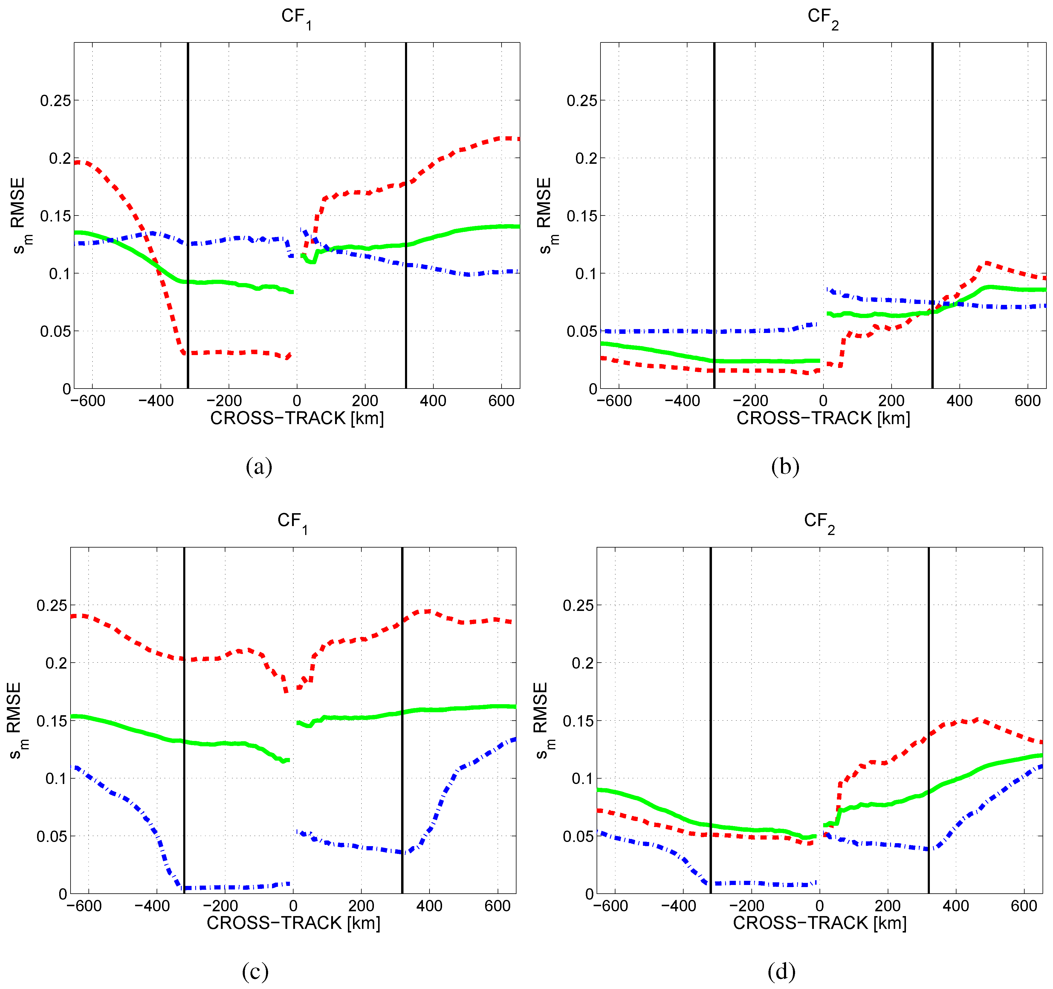
The use of adequate ancillary information on the cost function significantly improves the accuracy of $s_m$ retrievals, and is needed to satisfy the SMOS science requirement of 0.04 m${}^3$/m${}^3$. Using $C{F}_2$ constraints (Table 2), $s_m$ RMSE retrievals of ≈ 0.07 to 0.09 m${}^3$/m${}^3$ are obtained using $(T_{hh},T_{vv})$, and of ≈ 0.03 to 0.05 m${}^3$/m${}^3$ using $T_I$ over bare soil scenarios. As expected, there is a strong decrease of the brightness temperatures sensitivity to $s_m$ in the presence of vegetation, and $s_m$ RMSE retrievals of ≈ 0.11 to 0.13 m${}^3$/m${}^3$ are obtained using $(T_{hh},T_{vv})$, and of ≈ 0.05 to 0.09 m${}^3$/m${}^3$ using $T_I$ (with $\tau =0.24,\omega =0$).

–

The use of adequate constraints on the cost function ($C{F}_2$) highly improves the accuracy of τ estimations and is therefore critical to derive VWC maps from SMOS at the required accuracy of 0.2 kg/m${}^2$; Preliminary calculations indicate that VWC maps with an accuracy of ≈ 1.9 to 2.2 kg/m${}^2$ could be estimated from τ retrievals using $(T_{hh},T_{vv})$, and of ≈ 0.4 to 0.6 kg/m${}^2$ using $T_I$.

–

More accurate soil moisture estimates have been obtained over wet soils than over dry soils (bare and with low vegetation), except for the case of retrievals using $T_I$ and $C{F}_2$. Regarding τ retrievals, more accurate estimates have been obtained over wet soils than over dry soils in all the configurations.

–

Better $s_m$ retrievals have been obtained when using $T_I$ than when using $T_{hh}-T_{vv}$. Also, the formulation in terms of $T_I$ leads to better τ retrievals in all the configurations. These results suggest that, although $T_{hh}-T_{vv}$ is the formulation generally adopted in most studies, the use of $T_I$ should not be disregarded. In addition, $T_I$ is more robust in the presence of geometric rotations and Faraday rotation (at any spatial scale) than $(T_{hh},T_{vv})$. These effects have been perfectly corrected on the simulations, but are critical from an operational point of view.

–

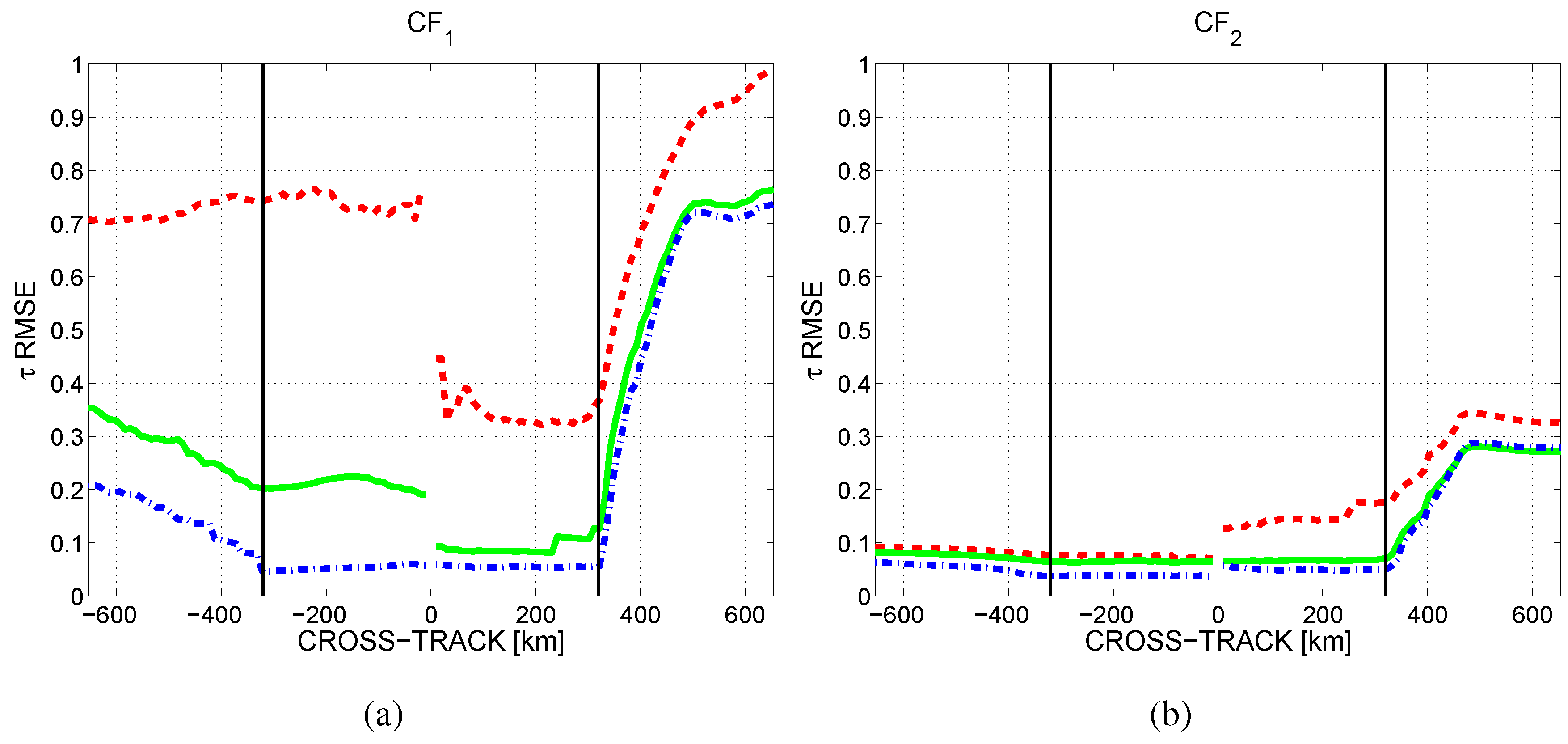
Due to SMOS observation geometry, better accuracies could be obtained if only the Narrow Swath (640-km, the central part of the FOV) is used. The use of adequate constraints ($C{F}_2$) and the retrieval formulation in terms of $T_I$ provide the most accurate $s_m$ and τ retrievals over all scenarios in the case of considering either the nominal or the Narrow Swath.

From an operational perspective, it should be pointed out that the forward model used in SEPS and in the L2 processor is not as complex as the one used in the ESA’s SMOS Level 2 Processor (the L-MEB model). The L2 processor uses the $\tau -\omega$ model, which is the core of the L-MEB model, and does not take into account any specific land cover parametrization for heterogeneous pixels. The main difference in the forward model is in the optical depth formulation, that in L-MEB is dependent on the incidence angle and the vegetation structure. In this study, it is considered that most vegetation covers are randomly oriented, and the optical depth parametrization has been simplified (see Section 2.2.). However, note that the optimization algorithm used in the L2 Processor Simulator is exactly as described in the SMOS Algorithm Theoretical Bases Document [23]. Thus, the results presented on this paper are potentially applicable to upcoming SMOS data and could timely contribute to the inversion of the very first SMOS observations during the calibration/validation phase.

Following the successful deployment of SMOS in orbit, continuous efforts will be needed to consolidate an optimal soil moisture retrieval configuration. The present study has analyzed the soil moisture inversion algorithm, both theoretically and in terms of performance with simulated data; it addresses key aspects for the retrieval of accurate soil moisture estimations, which are urgently needed to further our understanding of the Earth’s global water cycle and climate change impacts.

References

1. Entekhabi, D.; Asrar, G.; Betts, A.; Beven, K.; Bras, R. An agenda for land surface hydrology research and a call for the Second International Hydrological Decade. Bull. Amer. Meteor. Soc. 1999, 80, 2043–2058. [Google Scholar] [CrossRef]
2. Krajewski, W.; Anderson, M.; Eichinger, W.; Entekhabi, D.; Hornbuckle, B.; Houser, P.; Katul, G.; Kustas, W.; Norman, J.; Peters-Lidard, C.; Wood, E. A remote sensing observatory for hydrologic sciences: a genesis for scaling to continental hydrology. J. Water Resour. Res. 2006. [Google Scholar] [CrossRef]
3. Wagner, W.; Blsch, G.; Pampaloni, P.; Calvet, J.; Bizarri, B.; Wigneron, J.P.; Kerr, Y. Operational readiness of microwave remote sensing of soil moisture for hydrologic applications. Nord. Hydrol. 2007, 38, 1–20. [Google Scholar] [CrossRef]
4. Njoku, E.; Entekhabi, D. Passive microwave remote sensing of soil moisture. J. Hydrol. 1996, 184, 101–129. [Google Scholar] [CrossRef]
5. Schmugge, T.; Kustas, W.; Ritchie, J.; Jackson, T.; Rango, A. Remote sensing in hydrology. Adv. Water Resour. 2002, 25, 1367–1385. [Google Scholar] [CrossRef]
6. Ulaby, F.; Moore, R.; Fung, A. Microwave Remote Sensing Active and Passive, Vol. 1 and 2; Artech House: Norwood, MA, USA, 1981. [Google Scholar]
7. Shi, J.; Wang, J.; Hsu, A.; ONeill, P.; Engman, E.T. Estimation of bare surface soil moisture and surface roughness parameter using L-band SAR image data. IEEE Trans. Geosci. Remote Sens. 1997, 35, 1254–1266. [Google Scholar]
8. Jackson, T.; Schmugge, T.; Engman, E. Remote sensing applications to hydrology: soil moisture. Hydrol. Sci. J.-J. Des. Sci. Hydrol. 1996, 41, 517–530. [Google Scholar] [CrossRef]
9. Kerr, Y.; Waldteufel, P.; Wigneron, J.P.; Font, J.; Berger, M. Soil moisture retrieval from space: the soil moisture and ocean salinity (SMOS) mission. IEEE Trans. Geosci. and Remote Sens. 2001, 39, 1729–1735. [Google Scholar] [CrossRef]
10. National Research Council. Earth Science and Applications from Space: National Imperatives for the next Decade and Beyond; Technical report, Space Studies Board, National Academies Press: Washington, DC, WA, USA, 2007. [Google Scholar]
11. Martín-Neira, M.; Ribó, S.; Martín-Polegre, A.J. Polarimetric mode of MIRAS. IEEE Trans. Geosci. Remote Sens. 2002, 40, 1755–1768. [Google Scholar] [CrossRef]
12. Mission Objectives and Scientific Requirements of the SMOS Mission. MRD, version 5; Technical report, European Space Agency: Paris, France, 2003.
13. Pellarin, T.; Wigneron, J.P.; Calvet, J.; Waldteufel, P. Global soil moisture retrieval on a synthetic L-band brightness temperature data set. J. Geophys. Res. 2003, 108, 4364. [Google Scholar] [CrossRef]
14. Pardé, M.; Wigneron, J.P.; Waldteufel, P.; Kerr, Y. N-parameter retrievals from L-band microwave observatinos acquired over a variety of crop fields. IEEE Trans. Geosci. Remote Sens. 2004, 42, 1168–1178. [Google Scholar] [CrossRef]
15. Camps, A.; Vall-llossera, M.; Duffo, N.; Torres, F.; Corbella, I. Performance of sea surface salinity and soil moisture retrieval algorithms with different auxiliary datasets in 2-D L-band aperture synthesis interferometric radiometers. IEEE Trans. Geosci. Remote Sens. 2005, 43, 1189–1200. [Google Scholar] [CrossRef]
16. Wang, J.R.; Schmugge, T. An empirical model for the complex dielectric permittivity of soils as a function of water content. IEEE Trans. Geosci. Remote Sens. 1980, GRS-18, 288–295. [Google Scholar] [CrossRef]
17. Dobson, M.C.; Ulaby, F.T.; Hallikainen, M.T.; El-Rayes, M.A. Microwave dielectric behavior of wet soil-Part II: Dielectric mixing models. IEEE Trans. Geosci. Remote Sens. 1985, GE-23, 35–46. [Google Scholar] [CrossRef]
18. van de Griend, A.; Wigneron, J.P. The b-factor as a function of frequency and canopy type at H-polarization. IEEE Trans. Geosci. Remote Sens. 2004, 42, 786–794. [Google Scholar] [CrossRef]
19. Camps, A.; Corbella, I.; Vall.llossera, M.; Duffo, N.; Marcos, F.; Martinez-Fadrique, F.; Greiner, M. The SMOS end-to-end performance simulator: description and scientific applications. Proc. IEEE IGARSS 2003, 1, 13–15. [Google Scholar]
20. Talone, M.; Camps, A.; Mourre, B.; Sabia, R.; Vall-llossera, M.; Gourrion, J.; Gabarró, C.; Font, J. Simulated SMOS levels 2 and 3 products: the effect of introducing ARGO data in the processing chain and its impact on the error induced by the vicinity of the coast. IEEE Trans. Geosci. Remote Sens. 2009, 47, 3041–3050. [Google Scholar] [CrossRef]
21. Sabia, R.; Camps, A.; Talone, M.; Vall-llossera, M.; Font, J. Determination of sea surface salinity error budget in the soil moisture and ocean salinity mission. IEEE Trans. Geosci. Remote Sens. 2010, in press. [Google Scholar] [CrossRef]
22. Monerris, A. Experimental estimation of soil emissivity and its application to soil moisture retrieval in the SMOS mission. PhD thesis, Universitat Politècnica de Catalunya, Barcelona, Spain, 2009. [Google Scholar]
23. Algorithm Theoretical Bases Document; ATBD, Issue 3.a; Technical report; European Space Agency: Paris, France, 2007; Available online: http://www.cesbio.ups-tlse.fr/ (accessed on 10 December 2009).
24. Masson, V.; Champeaux, J.L.; Chauvin, F.; Meriguet, C. A global database of land surface parameters at 1-km resolution in meteorological and climate models. J. Climate 2003, 16, 1261–1282. [Google Scholar] [CrossRef]
25. Choudhury, B.; Schmugge, T.; Chang, A.; Newton, R. Effect of surface roughness on the microwave emission from soils. J. Geophys. Res. 1979, 84, 5699–5706. [Google Scholar] [CrossRef]
26. Mo, T.; Choudhury, B.; Schmugge, T.; Jackson, T. A model for microwave emission from vegetation-covered fields. J. Hydrol. 1982, 184, 101–129. [Google Scholar] [CrossRef]
27. Ulaby, F.T.; Wilson, A.E. Microwave attenuation properties of vegetation canopies. IEEE Trans. Geosci. Remote Sens. 1985, GE-23, 746–753. [Google Scholar] [CrossRef]
28. Wang, J.; Choudhury, B. Remote sensing of soil moisture content over bare field at 1.4 GHz frequency. J. Geophys. Res. 1981, 86, 5277–5282. [Google Scholar] [CrossRef]
29. Wigneron, J.P.; Laguerre, L.; Kerr, Y. A simple parameterization of the L-band microwave wmission from rough agricultural soils. IEEE Trans. Geosci. Remote Sens. 2001, 39, 1696–1707. [Google Scholar] [CrossRef]
30. Jackson, T.J.; Vine, D.M.L.; Hsu, A.Y.; Oldak, A.; Starks, P.J.; Swift, C.T.; Isham, J.D.; Haken, M. Soil moisture mapping at regional scales using microwave radiometry: the Southern Great Plains hydrology experiment. IEEE Trans. Geosci. Remote Sens. 1999, 37, 2136–2151. [Google Scholar] [CrossRef]
31. Wigneron, J.; Kerr, Y.; Waldteufel, P.; Saleh, K.; Escorihuela, M.-J.; Richaume, P.; Ferrazzoli, P.; Grant, J.P.; Hornbuckle, B.; de Rosnay, P.; Calvet, J.-C.; Pellarin, T.; Gurney, R.; Matzler, C. L-band Microwave Emission of the Biosphere (L-MEB) Model: description and calibration against experimental data sets over crop fields. Remote Sens. Environ. 2007, 107, 639–655. [Google Scholar] [CrossRef]
32. Panciera, R.; Walker, J.P.; Kalma, J.D.; Kim, E.J.; Saleh, K.; Wigneron, J.P. Evaluation of the SMOS L-MEB passive microwave soil moisture retrieval algorithm. Remote Sens. Environ. 2009, 113, 435–444. [Google Scholar] [CrossRef]
33. Saleh, K.; Kerr, Y.; Richaume, P.; Escorihuela, M.J.; Panciera, R.; Delwart, S.; Boulet, G.; Maisongrande, P.; Walker, J.P.; Wursteisen, P.; Wigneron, J.P. Soil moisture retrievals at L-band using a two-step inversion approach (COSMOS/NAFE’05 Experiment). Remote Sens. Environ. 2009, 113, 1304–1312. [Google Scholar] [CrossRef] [Green Version]
34. Schneeberger, K.; Schwank, M.; Stamm, C.; de Rosnay, P.; Mätzler, C.; Flühler, H. Topsoil structure influencing soil water retrieval by microwave radiometry. Vadose Zone J. 2004, 3, 1169–1179. [Google Scholar] [CrossRef]
35. Escorihuela, M.; Kerr, Y.; de Rosnay, P.; Wigneron, J.; Calvet, J.; Lemaitre, F. A simple model of the bare soil microwave emission at L-band. IEEE Trans. Geosci. Remote Sens. 2007, 45, 1978–1987. [Google Scholar] [CrossRef]
36. Kirdiashev, K.P.; Chukhantsev, A.A.; Shutko, A.M. Microwave radiation of the earth’s surface in presence of vegetation cover. Radio Eng. Elect. 1979, 24, 256–264. [Google Scholar]
37. Wigneron, J.P.; Chanzy, A.; Calvet, J.; Bruguier, N. A simple algorithm to retrieve soil moisture and vegetation biomass using passive microwave measurements over crop fields. Remote Sens. Environ. 1995, 51, 331–341. [Google Scholar] [CrossRef]
38. Hornbuckle, B.K.; England, A.W.; de Roo, R.D.; Fischman, M.A.; Boprie, D.L. Vegetation canopy anisotropy at 1.4 GHz. IEEE Trans. Geosci. Remote Sens. 2003, 41, 2211–2222. [Google Scholar] [CrossRef]
39. Owe, M.; de Jeu, R.; Walker, J.P. A methodology for surface soil moisture and vegetation optical depth retrieval using the microwave polarization difference index. IEEE Trans. Geosci. Remote Sens. 2001, 39, 1643–1654. [Google Scholar] [CrossRef]
40. Hornbuckle, B.K.; England, A.W. Diurnal variation of vertical temperature gradients within a field of maize: implications for stellite microwave radiometry. IEEE Geosc. Remote Sens. Lett. 2005, 2, 74–77. [Google Scholar] [CrossRef]
41. Jackson, T.; Schmugge, T. Vegetation effects on the microwave emission from soils. Remote Sens. Environ. 1991, 36, 203–212. [Google Scholar] [CrossRef]
42. Marquardt, D. An algorithm for least-squares estimation of nonlinear parameters. J. Soc. Ind. Appl. Math. 1963, 11, 431–441. [Google Scholar] [CrossRef]
43. Randa, J.; Lahtinen, J.; Camps, A.; Gasiewski, A.; Hallikainen, M.; Vine, D.L.; Martín-Neira, M.; Piepmeier, J.; Rosenkranz, P.; Ruf, C.; Shiue, J.; Skou, N. Recommended Terminology for Microwave Radiometry; Technical report; National Institution of Standards and Tecnology: Gaithersburg, MA, USA, 2008. [Google Scholar]
44. Piles, M.; Camps, A.; Vall-llossera, M.; Monerris, A.; Talone, M.; Sabater, J.M. Performance of Soil Moisture Retrievals using Multi-angular L-band Brightness Temperatures. Water Resour. Res. 2010, in press. [Google Scholar] [CrossRef]
45. Portabella, M.; Stoffelen, A. A probabilistic approach for seawinds data assimilation. Q. J. R. Meteorol. Soc. 2004, 130, 127–152. [Google Scholar] [CrossRef]
46. Gabarró, C.; Portabella, M.; Talone, M.; Font, J. Toward an Optimal SMOS Ocean Salinity Inversion Algorithm. IEEE Geosci. Remote. Sens. 2009, 6, 509–513. [Google Scholar] [CrossRef]
47. Davenport, I.J.; Fernandez-Galvez, J.; Gurney, R.J. A sensitivity analysis of soil moisture retrieval from the tau-omega microwave emission model. IEEE Trans. Geosci. Remote Sens. 2005, 43, 1304–1316. [Google Scholar] [CrossRef]
48. SEPS Architectural Detailed Design Document; ADDD V5.0; Technical report; European Space Agency: Paris, France, 2006; Available online: http://cassiopea.estec.esa.int/SEPS/Documents/ (accessed on 10 December 2009).
49. de Jeu, R.; Wagner, W.; Holmes, T.; Dolman, H.; van de Giesen, N.; Friesen, J. Global soil moisture patterns observed by space borne microwave radiometers and scatterometers. Surv. Geophys. 2008, 29, 399–420. [Google Scholar] [CrossRef]
50. Barre, H.M.J.; Duesmann, B.; Kerr, Y. SMOS: the mission and the system. IEEE Trans. Geosci. Remote Sens. 2008, 46, 587–593. [Google Scholar] [CrossRef]