
Monitoring of Atmospheric Carbon Dioxide over a Desert Site Using Airborne and Ground Measurements
by
 , ,
, ,
Qin Wang
1,
Farhan Mustafa
1 ,
,
Lingbing Bu
1,*,
Juxin Yang
2,
Chuncan Fan
2,
Jiqiao Liu
2 and
Weibiao Chen
2 1
Collaborative Innovation Center on Forecast and Evaluation of Meteorological Disasters, Nanjing University of Information Science and Technology (NUIST), Nanjing 210044, China
2
Key Laboratory of Space Laser Communication and Detection Technology, Shanghai Institute of Optics and Fine Mechanics, Chinese Academy of Sciences, Shanghai 201800, China
*
Author to whom correspondence should be addressed.
Remote Sens. 2022, 14(20), 5224; https://doi.org/10.3390/rs14205224
Submission received: 12 September 2022
/
Revised: 12 October 2022
/
Accepted: 17 October 2022
/
Published: 19 October 2022
Abstract
:Accurate monitoring of atmospheric carbon dioxide (CO2) is of great significance for studying the carbon cycle. Compared to ground observational sites, airborne observations cover a wider area, which help in effectively monitoring the distribution of CO2 sources and sinks. In this study, an airborne campaign was carried out in June and July 2021 to measure the atmospheric CO2 concentration over a desert site, Dunhuang, located in western China. The dry-air column-averaged CO2 mole fraction (XCO2) inversion results obtained from the Atmospheric Carbon Dioxide Lidar (ACDL) system were compared with the Orbiting Carbon Observatory 2 (OCO-2) retrievals, portable Fourier Transform Spectrometer (EM27/SUN) measurement results, and with the XCO2 estimates derived using the airborne Ultraportable Greenhouse Gas Analyzer (UGGA) and the Copernicus Atmosphere Monitoring Service (CAMS) model measurements. Moreover, the vertical CO2 profiles obtained from the OCO-2 and the CAMS datasets were also compared with the airborne UGGA measurements. OCO-2 and CAMS CO2 measurements showed a vertical distribution pattern similar to that of the aircraft-based measurements of atmospheric CO2. In addition, the relationship of atmospheric CO2 with the aerosol optical depth (AOD) was also determined and the results showed a strong and positive correlation between the two variables.

1. Introduction
Atmospheric carbon dioxide (CO2) is the most important anthropogenic greenhouse gas due to its significant contribution to global warming and climate change [1,2]. It plays a notable role in hydrology, sea ice melting, sea-level rise, and atmospheric temperature changes [3,4,5]. A continuous increase in the atmospheric CO2 concentration has been observed since the industrial revolution and this increment is largely contributed by anthropogenic activities such as fossil fuel burning, land-use changes, and cement production [6,7,8]. Knowledge of CO2 sinks, sources, and transport flux is critical for developing strategies aimed at stabilizing CO2 emissions and it requires continuous monitoring and assessment of atmospheric CO2 using current techniques and improved technologies [9]. Several ground stations, such as the stations within the Global Atmospheric Watch (GAW) network [10] and the Total Carbon Column Observing Network (TCCON) sites [11], are monitoring the atmospheric CO2 with great precision, however, these ground-based observations have some limitations [12,13]. For instance, the observations obtained from the GAW stations are representative of only lower atmosphere and both GAW and TCCON sites are not uniformly distributed and have limited spatial coverage [14]. Another source of monitoring atmospheric CO2 is space-borne observations. Satellites provide the most effective way to monitor atmospheric CO2 with great spatiotemporal resolutions [15]. Several satellites including the Greenhouse gases Observing SATellite (GOSAT) [16,17], the Orbiting Carbon Observatory 2 (OCO-2) [18,19], TanSat [20], GOSAT-2 [21], and OCO-3 [22] are orbiting around the Earth and are exclusively monitoring the concentration of atmospheric CO2. These satellites record the spectral radiance variation of sunlight reflected from the Earth’s surface through their passive spectrometers. The satellite-derived CO2 retrievals may contain larger uncertainties due to the presence of clouds, aerosols, and other artefacts [23]. Therefore, continuous evaluation of satellite-derived CO2 estimates is crucial when using multiple satellite CO2 measurements for joint flux inversion, and for establishing an accurate long-term atmospheric CO2 data record.
Passive spectrometers that rely on sunlight produce some spatiotemporal limitations such as the absence of nighttime and seasonal high-latitude measurements and retrieval errors due to clouds, aerosols, and complex terrains with rapidly changing surface reflectivity and elevation [9]. Several studies suggested that these limitations could be reduced by active remote sensing based on the Light Detection and Ranging (LIDAR) techniques [24,25,26,27]. The sensors used for active remote sensing provide their own radiation sources, which can be turned into target-specific absorption features of atmospheric molecule using the differential absorption lidar (DIAL) technique. An Integrated Path Differential Absorption (IPDA) lidar is a special DIAL that provides a weighted average measurement of the gas [9]. The IPDA lidar systems have been used by several researchers to monitor the concentration of CO2 in the atmosphere [26,28,29,30]. Several research institutes and organizations have carried out the feasibility and sensitivity analyses of space-borne monitoring of atmospheric CO2 using lidar systems. Under the Active Sensing of CO2 Emissions over Nights, Days, and Seasons (ASCENDS) mission, the National Aeronautics and Space Administration (NASA) involved several groups to develop IPDA lidar systems for monitoring atmospheric CO2 [31]. The objective of the ASCENDS mission included measuring the atmospheric CO2 a precision and accuracy of <0.3 ppm and 1.2 ppm, respectively, over Rail Road Valley using a space-based lidar system [32]. The NASA Langley Research Center (LaRC) significantly contributed to maturing high-energy pulsed lasers for CO2 and wind lidar transmitters based on a 2-µm laser technology [33]. Adopting the IPDA lidar technique, the German Aerospace Agency (DLR) also developed a 1.57-µm lidar system for monitoring atmospheric CO2 and the results from the developed instrument have been discussed in previous studies [34,35]. Following the United States and Germany, China has also developed its own DIAL system for monitoring atmospheric CO2. The initial results obtained from the newly developed Chinese lidar have been discussed in recent studies [29,36].
China is the largest CO2 emitting nation, with an approximately 30% contribution to the overall growth in the global carbon budget over the past 15 years [37]. The Chinese Government is aggressively working to reduce the CO2 emission per unit GDP by 60–65% relative to 2005 levels, and peak carbon emissions overall, by 2030 [14]. Continuous monitoring of atmospheric CO2 and evaluation of how well these reduction policies are working is hindered by larger uncertainties in the current datasets [38]. Therefore, it is necessary to evaluate the current CO2 datasets against precise and accurate measurements and monitor the atmospheric CO2 with improved technologies.
In this study, a combined ground-based and airborne experiment was carried out over a desert site, Dunhuang, located in western China. Airborne observations were measured using an IPDA lidar and a commercial instrument the UGGA, whereas, at the same time, the ground-based measurements of atmospheric CO2 were carried out using a portable Fourier Transform Spectrometer (EM27/SUN) and a separate UGGA. The results obtained from the airborne instruments were compared to ground-based measurements. Furthermore, the OCO-2 dataset was also validated against the ground-based and airborne measurements. In addition, the relationship between the atmospheric CO2 and the aerosols was also determined. The details about the airborne campaign and instrumentation, datasets, and ground-based site and instrumentation are given in Section 2. The results are discussed in Section 3 and the conclusions are given in Section 4.
2. Materials and Methods
China has developed an IPDA-based atmospheric carbon dioxide lidar (ACDL) system for monitoring atmospheric CO2 [28,29,30,36]. The ACDL has working wavelengths of 532, 1064, and 1572 nm. The 1572 nm channel is used for the IPDA technique to measure atmospheric CO2, whereas the 532 and 1064 nm channels are used to detect aerosols and clouds. More details about the ACDL are given in our previous study [29]. A series of airborne campaigns was planned to evaluate the performance of the ACDL system. The first airborne experiment was carried out in March 2019 over the Shanhaiguan area, located in northeast China. The observations were carried out over different types of surfaces including mountains, ocean, and urban areas and the results were compared with in situ and satellite measurements. The results of the first airborne campaign have been discussed in several studies [29,36]. This second airborne experiment was carried out to study the distribution of atmospheric CO2 and performance evaluation of the ACDL over a desert site in summer. The details about the experiment site, aircraft, and ground site instrumentations are given in the following.
2.1. Aircraft Instrumentation
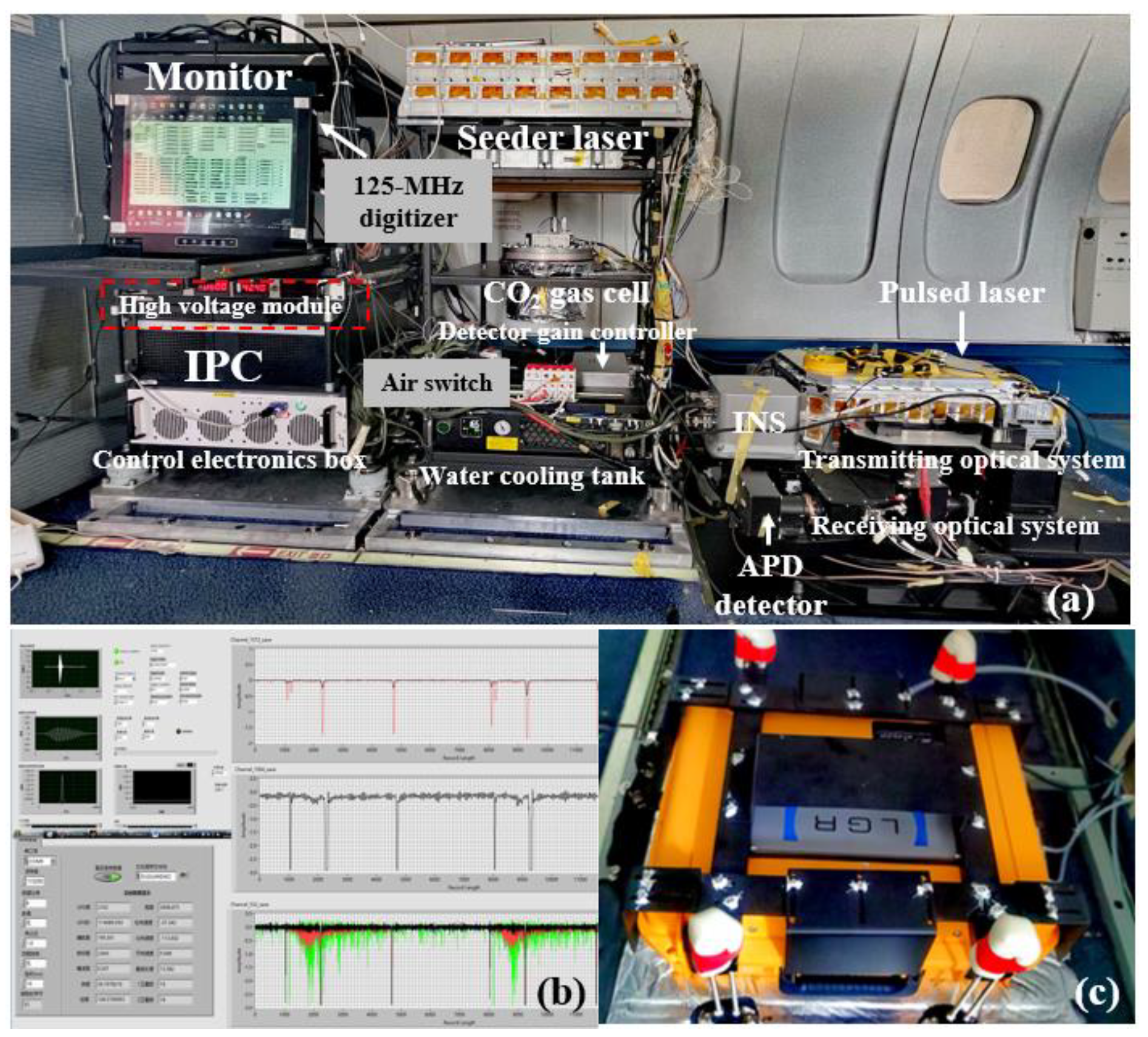
The aircraft used in the airborne experiment was the B-602K, which had a maximum cruising speed of 514 km/h. The aircraft was equipped with the ACDL system and a UGGA to measure the concentration of atmospheric CO2. The airborne equipment is shown in Figure 1. The ACDL system consisted of a laser transmitter, instrument control, environmental control, and a Light Detection and Ranging (LIDAR) transceiver subsystem. The description of each of the ACDL subsystems is provided in a previous study [29]. Furthermore, the UGGA was also installed on the aircraft and a 1/4-inch Teflon pipe was used to connect it with the external atmosphere. The UGGA uses a laser absorption technology known as the off-axis Integrated Cavity Output Spectroscopy (ICOS) to measure trace gas concentration in dry mole fraction with a high precision of <0.30 ppm for CO2 and <2 ppb for CH4 (UGGA user manual; model 915-0011; Los Gatos Research, San Jose, CA, USA). More technical information about the off-axis ICOS spectroscopy is provided in previous studies [39,40].
2.2. Ground Site
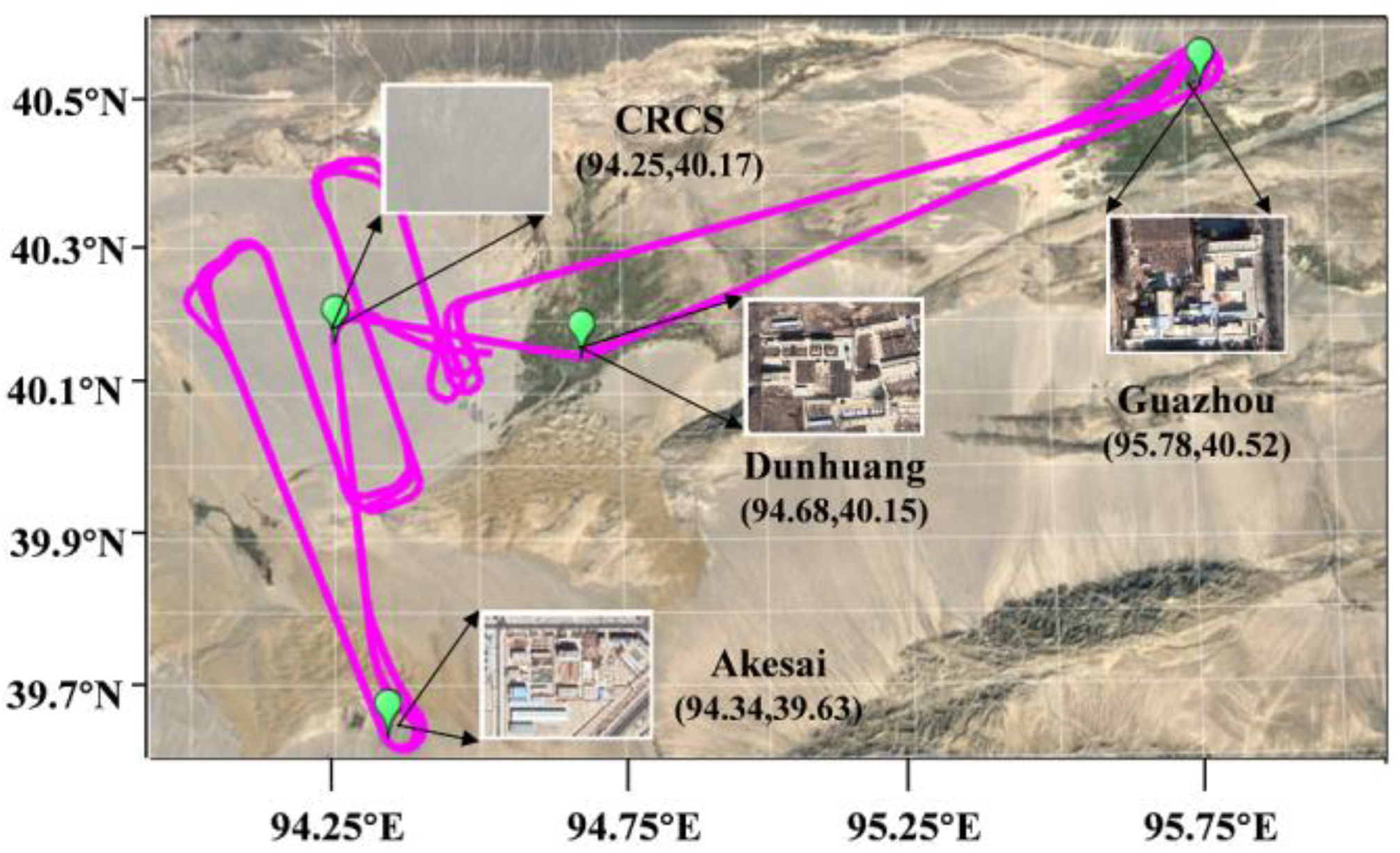
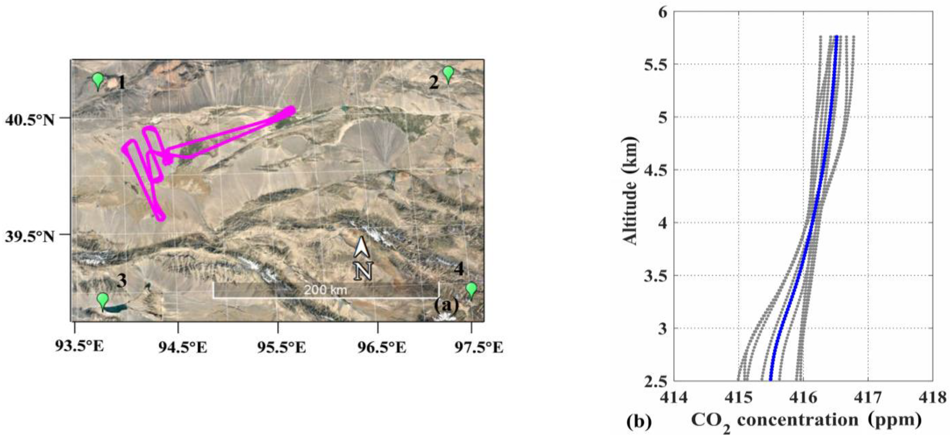
During the observation experiment, four ground stations were deployed at the experimental site. According to the observation requirements, different types of equipment were installed and configured at the ground stations. The four ground stations included the Dunhuang Meteorological Bureau, the Akesai Meteorological Bureau, the Guazhou Meteorological Bureau, and the Chinese Radiometric Calibration Site (CRCS). The locations of the ground stations are shown in Figure 2 and more details about the instruments installed at each of the stations are provided in Table 1.
The CRCS station was equipped with various instruments including atmospheric CO2 monitoring equipment such as EM27/SUN spectrometer and portable UGGA. Atmospheric CO2 monitoring instruments were installed over the CRCS station due to several reasons; (1) the CRCS ground station was located on a stable alluvial fan whose surface consisted of cemented gravel, some black or grey stones, and sand without any vegetation. It had the least human activity with no obvious anthropogenic emission sources. (2) The aircraft performed spiral and U-shaped flights at different altitudes over the CRCS ground station to obtain the vertical profiles of atmospheric CO2. It was convenient to compare and verify the observation results of airborne observations against the ground-based measurements. Furthermore, the other stations were deployed in the path of the airborne flight and instruments were installed at these stations to obtain the aerosol and meteorological data.
2.3. Flight Campaign
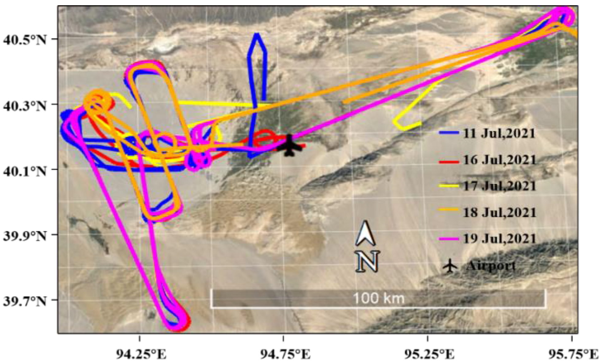
The airborne campaign was carried out from 11 to 19 July 2021 over a desert site, Dunhuang, located in western China. The objectives of the campaign included gaining a better understanding of the distribution characteristics of atmospheric CO2 in the desert area of western China in the summer and a performance evaluation of the ACDL system over a desert site. Flight paths of the airborne campaign are shown in Figure 3 and relevant details are given in Table 2.
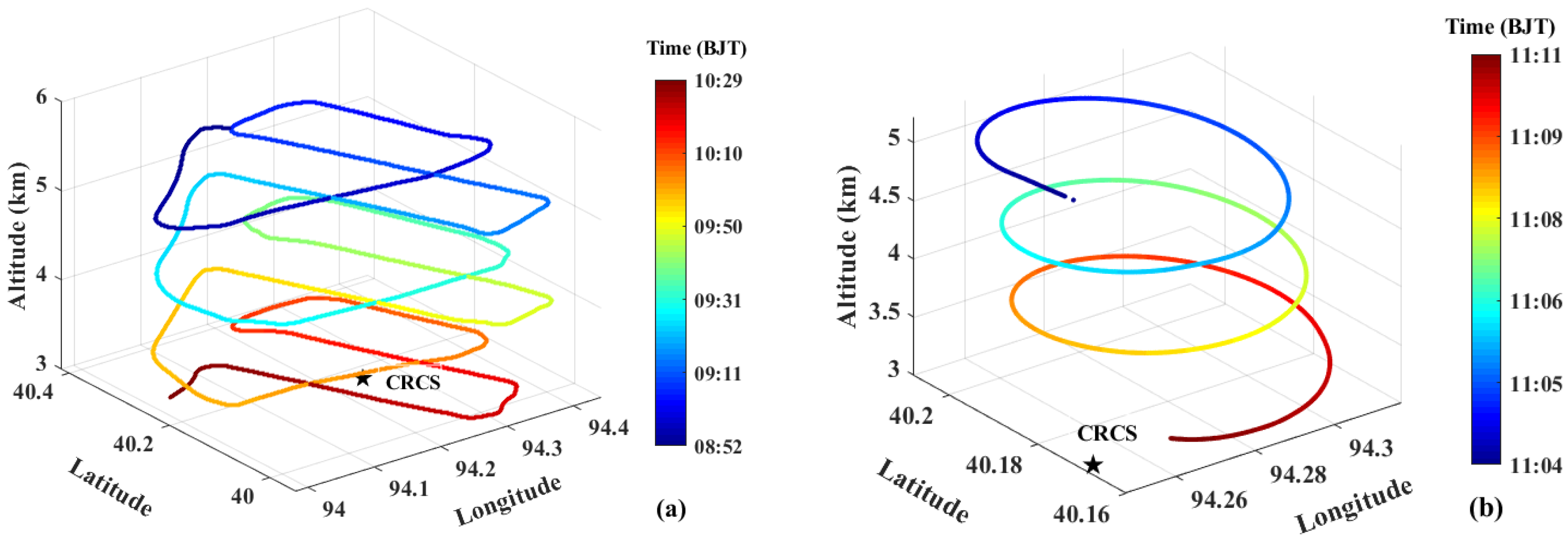
Three modes of flight were performed during the airborne observation experiment to get various kinds of data. (1) Long-term horizontal flight was carried out between the altitudes of 5 to 6 km to study the distribution characteristics of atmospheric CO2 in the troposphere. (2) U-shaped flight was performed at different heights over the CRCS ground station so that the lidar could obtain XCO2 information at different altitudes. (3) Spiral descent and ascent flight were also carried out over the CRCS station to get the vertical profiles of atmospheric CO2. This spiral flight mode can obtain the distribution characteristics of CO2 concentration at different altitudes, providing an important reference for validating the model and passive remote sensing measurement results. The U-shaped and spiral mode of flights was performed over the CRCS ground site so that results from the airborne observations could be compared with the ground-based atmospheric CO2 measurements. The U-shaped and spiral flight patterns on 11 July 2021 are shown in Figure 4. Restricted by the safe flight height, the aircraft could not land at a very low altitude for measurement. The minimum flight altitude was about 3 km.
2.4. Datasets
2.4.1. Airborne and Ground Station Data
A variety of data measured from the ground stations and airborne flights were used in this study. The major data obtained from the aircraft flights included the ACDL observations, which were used to estimate the XCO2 and in situ CO2 dry-air mole fraction of CO2 which were measured using the UGGA. However, some auxiliary data such as longitude, latitude, and altitude were also measured using the Inertial Navigation System (INS) installed on the aircraft. Furthermore, color photos of the surface were also obtained using a Complementary Metal Oxide Semiconductor (CMOS) camera (model: IDS ui-3360cp-c-hq Rev.2) with a resolution of 2048 × 1088 pixels, which was installed on the aircraft next to the lidar telescope. Ground-based XCO2 and in situ CO2 dry-air mole fraction of CO2 were obtained using the EM27/SUN spectrometer and UGGA, respectively, installed at the CRCS station. In addition, the aerosol optical depth and meteorological data were also measured using the instruments installed on various ground stations.
2.4.2. OCO-2 XCO2 Dataset
The Orbiting Carbon Observatory 2 (OCO-2) is a satellite launched by NASA on 2 July 2014 for the exclusive monitoring of atmospheric CO2 to get a better understanding of regional and global carbon cycles [18,19]. The sun-synchronous, near-polar satellite incorporates three high-resolution spectrometers making coincidental measurements of reflected sunlight in near-infrared CO2 near 1.61 and 2.06 µm and molecular oxygen (O2) A-Band at 0.76 µm with a temporal resolution of 16 days, allowing for the complete global coverage of XCO2 twice per month [41]. OCO-2 observations have been processed using various algorithms, however, the official OCO-2 XCO2 product is generated using the Atmospheric CO2 Observations from Space (ACOS) Full Physics (FP) retrieval algorithm [42,43]. OCO-2 XCO2 products have been continuously validated against the ground-based TCCON measurements and the results showed that the OCO-2 datasets were consistent and reliable for regional-scale monitoring of atmospheric CO2 [44,45]. In this study, we used the ACOS/OCO-2 XCO2 Level 2 Lite product v10r.
2.4.3. CAMS Model CO2 Dataset
The Copernicus Atmosphere Monitoring Service (CAMS) is an atmospheric analysis service providing spatiotemporal variations of atmospheric compositions including chemical species, aerosols, and greenhouse gases [46,47]. The CAMS analysis is produced using the ECMWF four-dimensional variational (4DVar) system [48] within the Integrated Forecasting System (IFS; version CY42r1 for 2016 and CY43r1 for 2017), which is one of the world’s leading operational global weather prediction systems [49]. Transport of tracers such as CO2 is carried out online by the IFS model concurrently with the meteorological forecast. In this study, we used the CAMS reanalysis product (v20r1) that provided the CO2 concentrations at a global scale with a spatial resolution of 1.9° × 3.8° (Lat × Lon) and a temporal resolution of 3 h. The referenced product provided the CO2 mole fractions at 39 vertical levels from the Earth’s surface to higher than 70 km. In this study, the model-derived CO2 mole fractions were spatiotemporally interpolated to the study area.
2.5. Data Analysis
The solar spectra measured by the EM27/SUN spectrometer were used to estimate the using the PROFFAST software, similar to a previous study [50]. Furthermore, to estimate from the airborne UGGA observations, the missing profiles were first extrapolated to the whole atmosphere using a method suggested by Ref. [44] and then was estimated using Equation (1), which was given in previous studies [51,52]:
where is the calculated from the aircraft measurement or model, is the column-averaged dry air mole fraction for the a priori profile , is the pressure weighting function, is the column averaging kernel, and is the CO2 profile measured from the aircraft or model. from the model measurements were also estimated using Equation (1). Moreover, from the ACDL system were derived using the method given in Section 4.2 of our previous study [29].
3. Results
3.1. Diurnal Variations of Atmospheric CO2
The diurnal variations of atmospheric CO2 were measured over the CRCS ground station using the portable EM27/SUN spectrometer and UGGA. The hourly-averaged diurnal XCO2 estimated from the EM27/SUN spectrometer observations and in situ CO2 measurements obtained from the UGGA, respectively, are shown in Figure 5 and Figure 6.
The EM27/SUN was operating on sunny days from 26 June to 19 July 2021, whereas, UGGA operated from 2 July to 19 July 2021. To maintain the quality of the results, the observations influenced by bad weather were discarded. The highest daily mean XCO2 concentration of 414.63 ± 0.11 ppm was reported on 26 June 2021 and this concentration decreased and reached the minimum (411.06 ± 0.30 ppm) on 7 July 2021. It started to increase again, reaching the second peak (413.97 ± 0.40 ppm) on 12 July 2021, and after that it started decreasing again. Similar results were observed from UGGA in situ measurements. The daily mean concentration of atmospheric CO2 was lower (404.93 ± 1.20 ppm) on 5 July 2021 and then it started increasing and reached the peak (408.35 ± 0.18 ppm) on 13 July 2021 and, after that, it started decreasing again. On the morning of 5 July 2021, the wind direction at Dunhuang was northerly. As can be seen from the geographic location in Figure 2, there is a large desert uninhabited area to the north of the CRCS ground station, so the CO2 released by the respiration of animals and plants at night cannot be transported to the CRCS ground station. In addition, the weather was sunny on 5 July 2021. After sunrise, plants in the surrounding oases (in and around Dunhuang City) start photosynthesizing and begin to consume the CO2 accumulated in the atmosphere overnight. So, the CO2 in the morning on 5 July 2021 has a big reduction. The hourly-averaged concentrations of atmospheric CO2 obtained from the EM27/SUN spectrometer (Figure 5) and the UGGA (Figure 6) showed a sinusoidal pattern. The results are in agreement with a previous study [12]. The atmospheric CO2 concentration gradually decreased from 8:00 h to 9:00 h (17 July 2021) or to 10:00 h (11, 16, and 18 July 2021). After that the value reversed and started to rise, reaching the first peak at 13:00 h or 14:00 h (Solar noontime of ~13:45 h at Dunhuang). After 13:00 h, the concentration of CO2 began to decrease again during the period until 17:00 h, and after that, it rose again after 17:00 h. In addition to the disturbance of human activities, light and temperature are also among the main factors that significantly contribute to this change. For instance, after sunrise, plants in the surrounding oases (in and around Dunhuang City) start photosynthesizing and begin to consume the CO2 accumulated in the atmosphere overnight. However, as the ambient temperature increases (the ambient temperature in Dunhuang may exceed 30 °C after 11:00 in July), the plants in the oasis will close their stomata to prevent water evaporation and reduce photosynthesis efficiency [53]. At this time, human activities become more and more frequent, which eventually leads to an increase in the concentration of CO2 in the atmosphere. In the afternoon, due to the reduction of human activities caused by high temperature and the recovery of photosynthesis of nearby plants, the concentration of CO2 in the atmosphere decreases slightly again. After 17:00 h, the CO2 concentration in the atmosphere increases again due to the recovery of human activities and the reduction of plant photosynthesis.
3.2. Vertical Variations of Atmospheric CO2
The vertical CO2 profiles were obtained during the U-shaped and spiral modes of the flights using the portable UGGA installed on the aircraft. The portable UGGA was calibrated against the standard gases before each flight experiment. The concentration of the standard gas used in this calibration was 382.15 ppm. The measurements of the standard CO2 concentration were carried out for a period of 3 min before and after the calibration of the instrument and the results are shown in Figure 7. It is evident from the results that the UGGA showed improved results after the calibration.
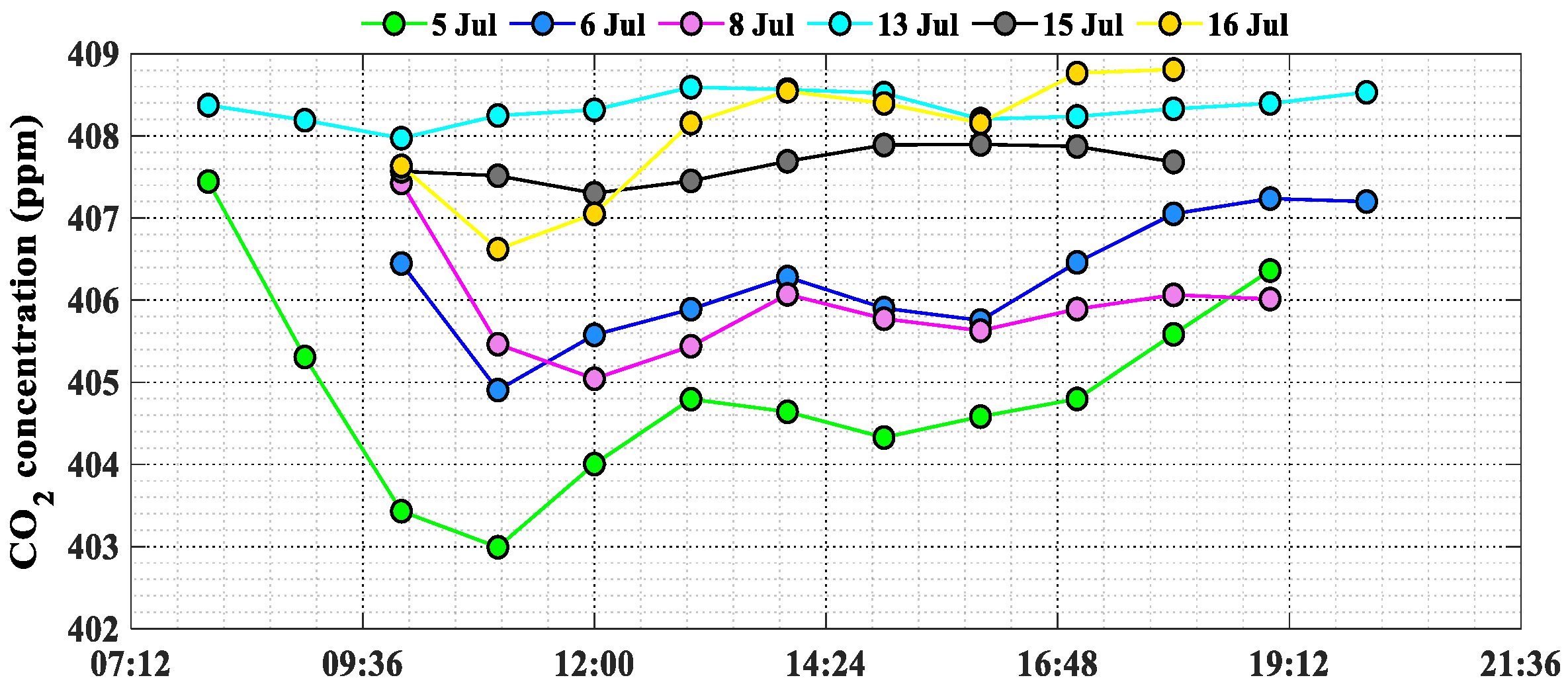
The vertical distribution of atmospheric CO2 measured using the portable UGGA is shown in Figure 8. The referenced figure is distributed into two sections. The first section (a) shows the CO2 concentration for several days against time and height. The descents and ascents of the aircraft are marked with orange and blue shadings, respectively. The highest mean CO2 concentration with a value of 413.49 ± 3.97 ppm was observed on 18 July 2021 and its maximum value reached 421.63 ppm at a height of around 6 km. However, the smallest mean CO2 concentration reported on 19 July 2021 had a value of 406.73 ± 1.18 ppm. The smallest value was observed near the surface. Figure 8b shows 10 s-averaged atmospheric CO2 mole fractions against height for several days. The vertical profiles of atmospheric CO2 for each day are shown in grey color. All of the CO2 vertical profiles are averaged to get an overall distribution trend and the results are shown as blue scatter points in Figure 8b. The results from Figure 8 show that the concentration of atmospheric CO2 is low near the surface and it gradually increases with the progression in the altitude. Restricted by the minimum flight safety altitude of the aircraft, atmospheric CO2 vertical structure was not measured to the ground. However, at an altitude is 2.91 km, the averaged CO2 concentration was 405.28 ppm and at an altitude of 5.11 km, the averaged CO2 concentration was 411.48 ppm. Generally, the concentration of atmospheric CO2 is higher near the surface. The contradiction observed in these results might be due to several reasons; (1) the experimental site had very limited human activity and no anthropogenic emissions, which significantly contributes to atmospheric CO2 concentration, and (2) the photosynthesis of vegetation in the near-surface Dunhuang area and nearby oasis may have led to a low CO2 concentration near the surface.
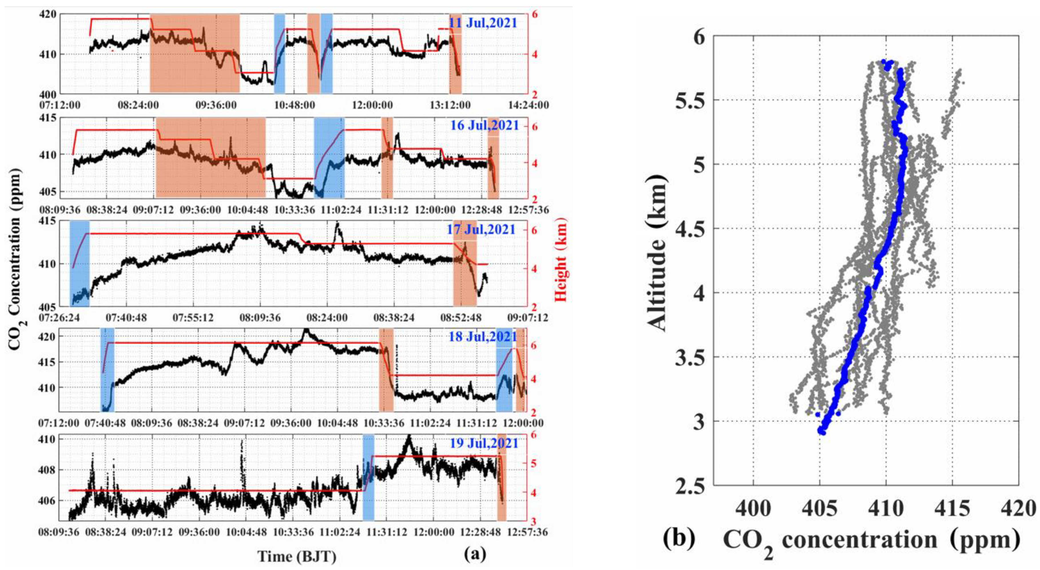
The vertical CO2 profiles obtained from OCO-2 and CAMS model datasets were also validated against airborne in situ CO2 observations. CAMS CO2 measurements were spatiotemporally interpolated to the experiment location and time. In the case of OCO-2, the data closer to the experimental site were observed on 16 and 18 July 2021, which was used in the study. OCO-2 satellite was passed closer to the experiment site at 14:53 and 14:41 h (CST) on 16 and 18 July 2021, respectively. The locations of OCO-2 and CAMS measurements closer to the experimental site and the vertical CO2 profiles obtained from these two datasets are shown in Figure 9 and Figure 10, respectively.
OCO-2 and CAMS CO2 vertical profiles were compared against in situ CO2 observations and the results are shown in Figure 11. Both OCO-2 and CAMS datasets also showed a lower atmospheric CO2 concentration near the surface and a comparatively higher concentration at higher altitudes exhibiting a similarity with airborne in situ observations. However, some differences were observed in the magnitudes of satellite and model datasets against in situ observations. Both satellite and model datasets were overestimated relative to in situ observations. Mustafa [14] compared the CO2 vertical profiles obtained from the OCO-2 dataset and reported an overestimation over Qinhuangdao, China. CAMS CO2 measurements were comparatively more overestimated, and this overestimation might be due to differences in spatial resolution and the presence of uncertainties in the input datasets that drive the model. Furthermore, the change in averaged CO2 concentration with respect to the pressure was also calculated for the datasets (Figure 11b) and the change rates of, 0.031, 0.025, and 0.004 ppm/hPa were observed for in situ, satellite, and model datasets, respectively.
3.3. XCO2 Estimation and Comparison
XCO2 results retrieved using the ACDL observations were compared to those obtained from a satellite, OCO-2, a model, CAMS, and airborne UGGA in situ measurements. The comparison results are given in Table 3. From the comparison results in Table 3, it can be seen that the XCO2 value of the IPDA lidar inversion is the smallest. The XCO2 result retrieved by the airborne UGGA during the spiral on 16 July 2021 is 1.71 ppm larger than the IPDA lidar result. The XCO2 value calculated by the CAMS mode is the largest and the XCO2 values on 16 July and 18 July 2021 are 416.03 ppm and 416.04 ppm, respectively. XCO2 retrieved by CAMS were comparatively more overestimated and this overestimation might be due to differences in spatial resolution. The difference between the ground-based EM27/SUN and OCO-2 measurements is 2.04 ppm on 18 July 2021. The previous research showed that at an altitude of about 3 km, the XCO2 results retrieved from the airborne in situ measurements are approximately 4 ppm larger than the airborne IPDA lidar measurements during the Science Flight 1 (SF1) in 2014 [54].
3.4. Relationship between XCO2 and Aerosols
The backscatter profiles and the aerosol optical depth (AOD)—although not used directly in the XCO2 retrieval—provide an important context for interpreting the retrieved XCO2 measurements. These variables can be used to identify clouds for retrieving partial column XCO2 to cloud tops [27]. Moreover, they also provide help in identifying and profiling smoke plumes from wildfires and assessing their impact on XCO2 [55]. In this section, we have determined the relationship of atmospheric XCO2 concentration with the aerosol optical depth using ground-based and airborne observations.
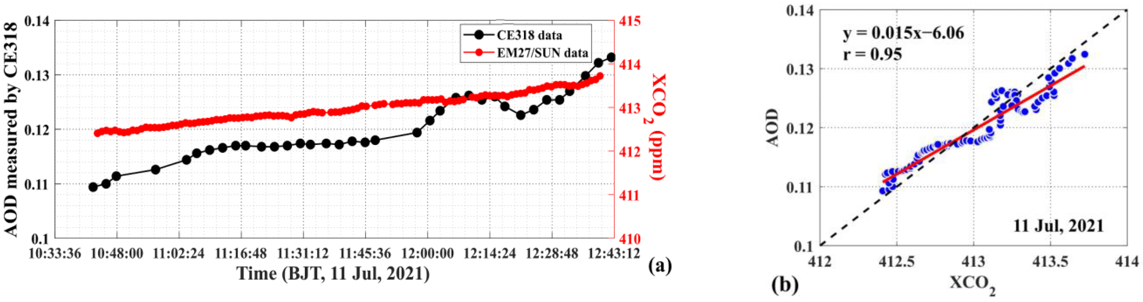
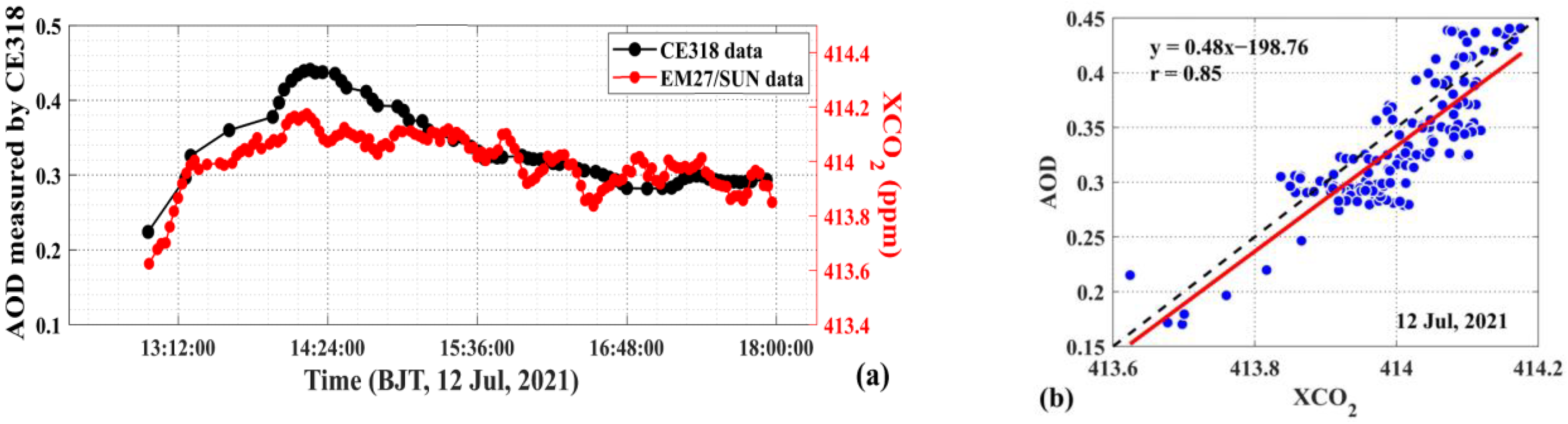
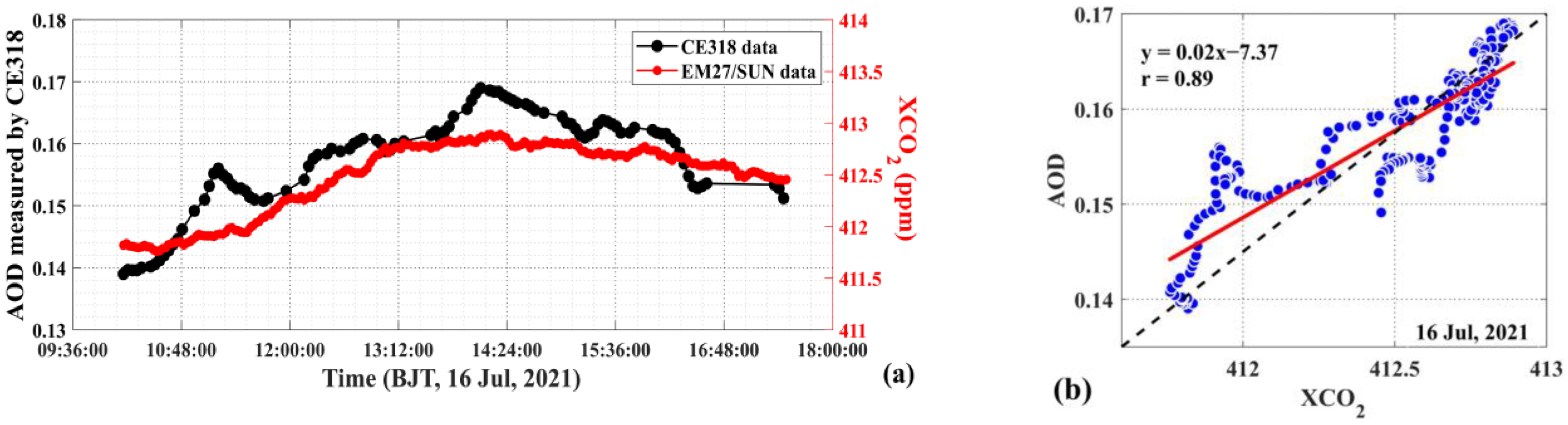
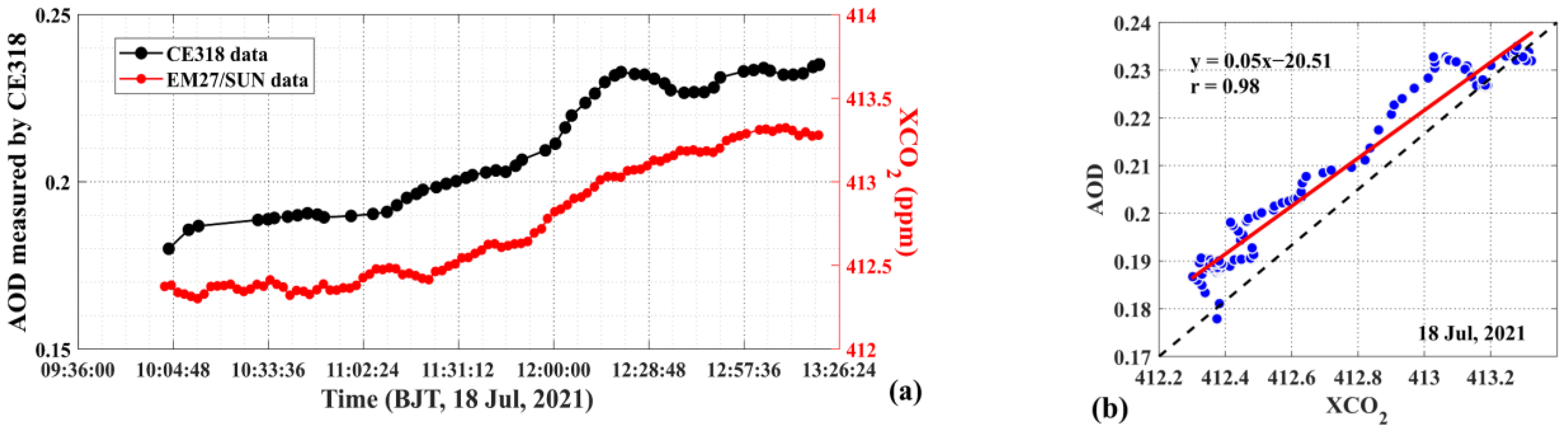
The XCO2 and the AOD were derived using the observations obtained from the EM27/SUN spectrometer and solar photometer CE318, which were installed at the CRCS ground station. Observations for four days, 11 July, 12 July, 16 July, and 18 July 2021, were used in this analysis. The relationship between the two variables was studied by carrying out trend and correlation analyses. The results from the trends and correlation between the AOD and XCO2 concentration for several days are given in Figure 12, Figure 13, Figure 14 and Figure 15.
The results from the referenced figures show a direct relationship between the two variables by exhibiting similar variation trends and strong and positive correlation coefficients. The lowest (r = 0.85) and the highest (r = 0.98) correlations between the diurnal XCO2 and AOD were observed on 12 July and 18 July 2021, respectively. The results from Figure 12, Figure 13, Figure 14 and Figure 15 show that higher values of XCO2 and AOD were observed during the day, from 11:00 to 15:00 h, and the values of these variables started decreasing after that. These diurnal changes can be associated with anthropogenic activities, which are lower in the mornings and evenings and higher during other times of the day. Furthermore, the boundary layer also contributes to the stronger relationship between AOD and XCO2 because the pollutants and the greenhouse gases cannot escape through the boundary layer. The microorganism activity, which increases with the temperature, contributes to atmospheric CO2 and polluting variables and it might also have a contribution to the higher values of AOD and XCO2 during the daytime.
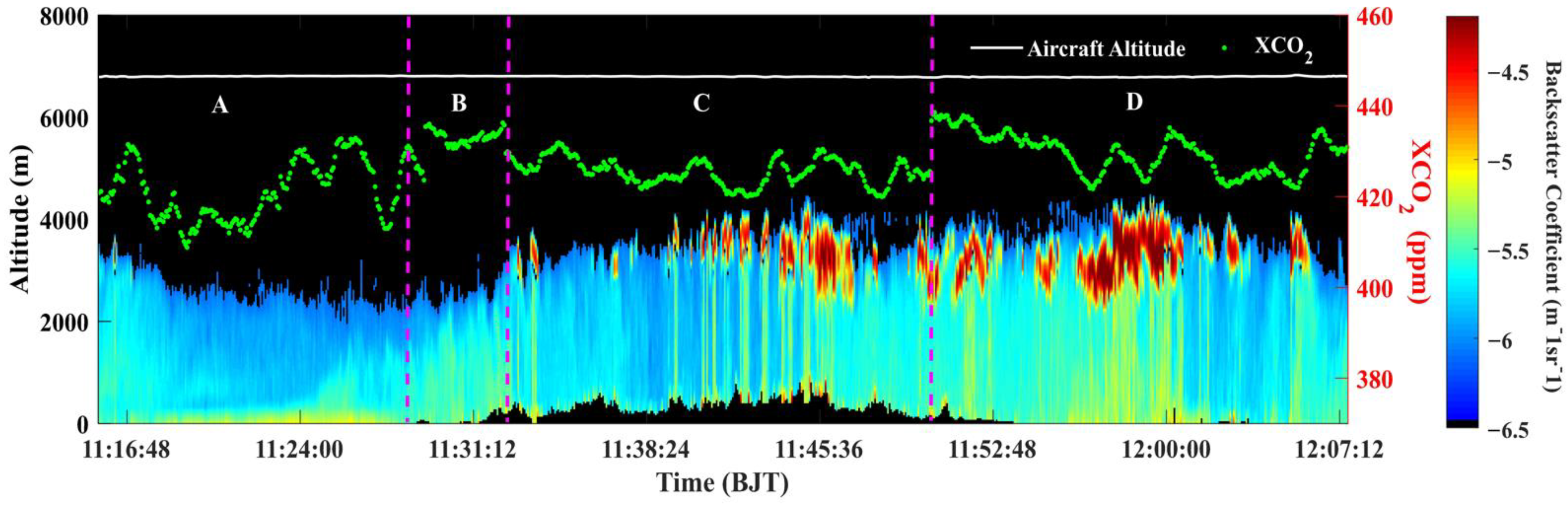
The relationship of atmospheric CO2 with AOD was also studied using airborne measurements. For that purpose, XCO2 and AOD were estimated using the ACDL system. The airborne ACDL system can simultaneously observe the distribution characteristics of aerosol and CO2 concentrations over a larger area. More importantly, airborne observations can measure the variations over various types of surfaces simultaneously. The current airborne experiment was carried out over desert areas. However, the previous airborne experiment was carried out over various types of surfaces including urban areas, mountains, and ocean located in Shanhaiguan, China. Therefore, to get a better understanding of aerosol and atmospheric CO2 over different surfaces, the measurements obtained from the previous experiment were used in this study. The aerosol backscattering coefficient measured by the airborne ACDL system and the inversion results of XCO2 distribution are shown in Figure 16.
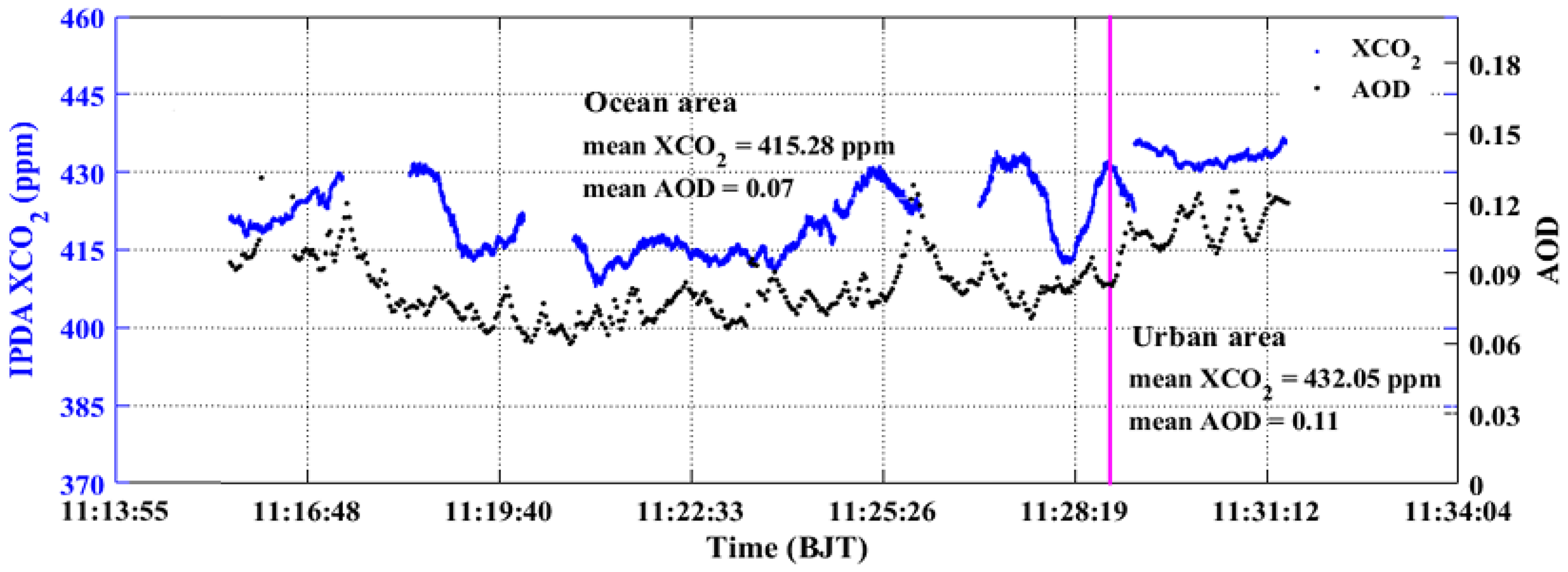
On 14 March 2019, the aircraft flew horizontally at an altitude of 6.8 km. In Figure 16, stages A–D represent the ocean, urban, mountain, and urban surface types, respectively. From the distribution of aerosol backscattering coefficients, it can be seen that there were clouds at a height of about 3.6 km after 11:32 h. Over the open ocean area (stage A), about 30 km away from the coastline, aerosols were mainly concentrated in the lower atmosphere, i.e., below 500 m in height. After 11:24, the aircraft began to fly from the far-sea area to the urban areas (stage B). Affected by human activities in the city, the atmospheric-planetary boundary layer gradually increased, and the aerosol backscattering coefficient became larger. Over the mountainous area (stage C), the aerosol backscattering coefficient was slightly lower than that of stage B. When the aircraft reached stage D, the measured aerosol backscattering coefficient became larger again. Correspondingly, the XCO2 value measured by the airborne ACDL was the smallest over the ocean (stage A). XCO2 gradually increased over the urban area (stage B) and reached the maximum value. To determine the consistency of AOD and XCO2 distributions, the aerosol optical parameters measured by the ACDL system were converted to AOD for comparison. Further, to remove the interference of cloud to AOD, only the results of stages A and B were selected for comparison, and the comparison results are shown in Figure 17.
Similar to the results obtained from the CRCS ground station measurements, airborne AOD and XCO2 also showed a good agreement across different surface types. The results from Figure 17 show that the values of XCO2 and AOD were the smallest over the ocean. The average value of XCO2 and AOD over the ocean was 415.8 ppm and 0.07, respectively. A gradual increase was observed in the values of both variables when the aircraft flew from the ocean to the urban area and reached the maximum values. The averaged XCO2 and AOD over the urban area were 432.05 ppm and 0.11, respectively.
4. Discussion
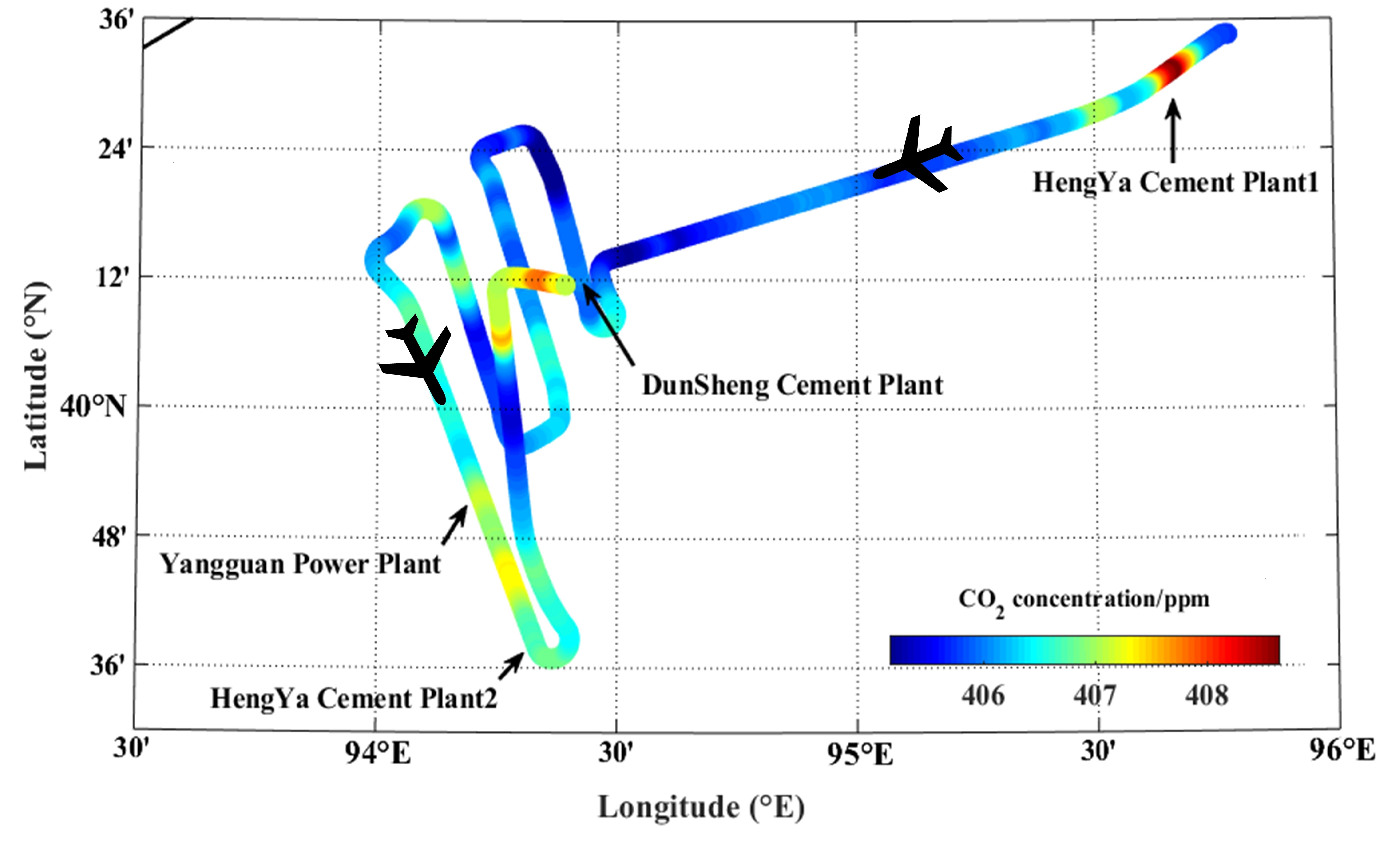
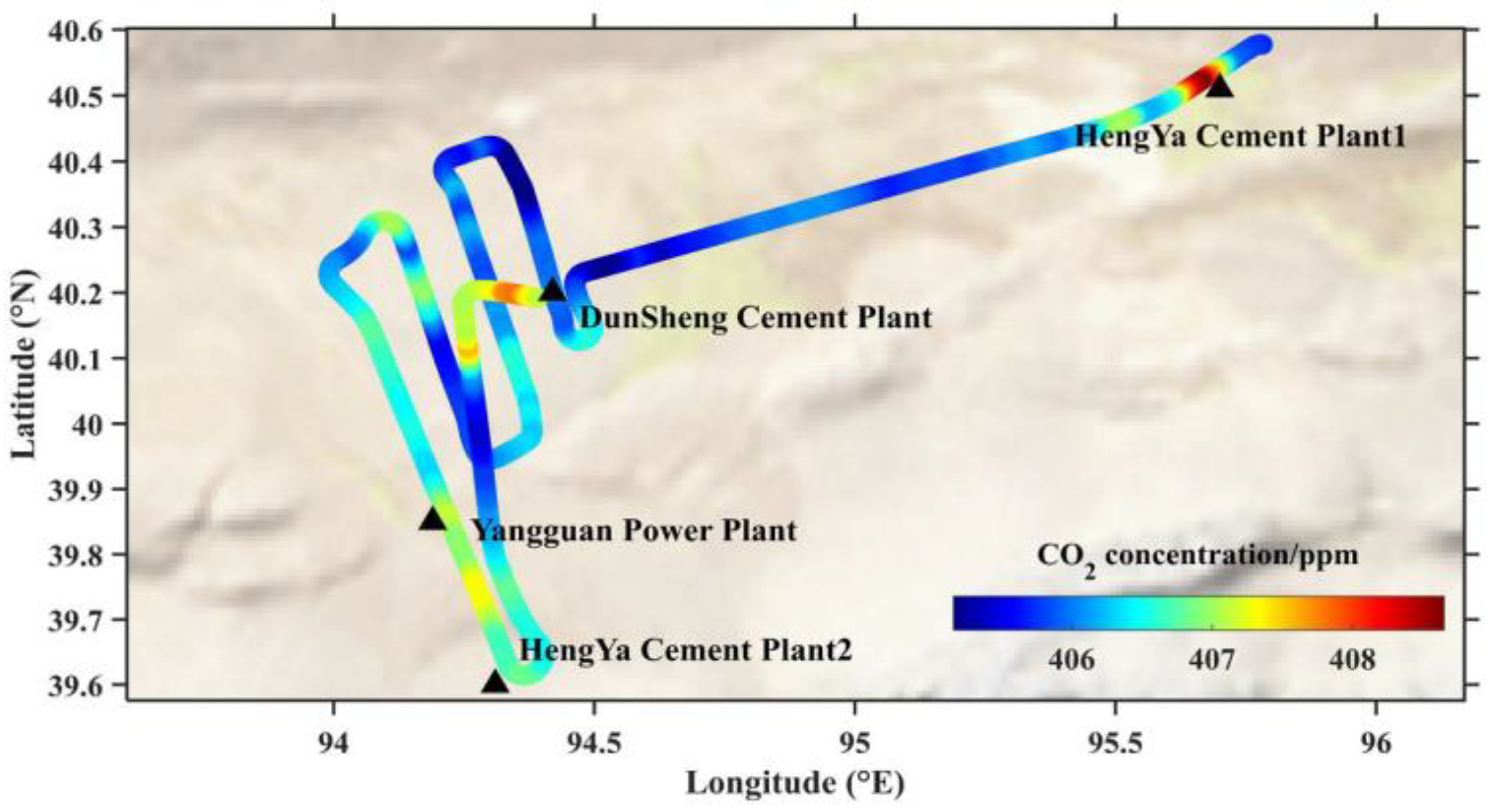
The hourly-averaged diurnal XCO2 estimated from the EM27/SUN spectrometer observations and in situ CO2 measurements obtained from the UGGA were analyzed. If the weather conditions are bad, our equipment will not be powered on for observation, so the effective data time periods under different weather conditions are different. The hourly-averaged concentrations of atmospheric CO2 obtained from the EM27/SUN spectrometer and the UGGA showed a sinusoidal pattern, similar to the observations (especially 26 and 28 March 2008) at the Jet Propulsion Laboratory (JPL) in the South Coast Air Basin (SCB) of California, USA [56]. In addition to the disturbance of human activities, light and temperature are also among the main factors that significantly contribute to this change. U-shaped and spiral flight were also carried out to obtain the distribution characteristics of CO2 concentration at different altitudes, providing an important reference for validating the model and passive remote sensing measurement results. The accurate detection of carbon sources and sinks is of great significance for the study of carbon transport and carbon cycle. Compared with ground station detection, airborne observation can realize the observation of a large area in a short time, and can cover a variety of surface types at the same time. It is one of the most effective ways of carbon source and sink detection. The results of atmospheric CO2 concentration measured by airborne UGGA during the plane’s horizontal flight at an altitude of 4.05 km on 19 July 2021 are shown in Figure 18. CO2 emission sources on the flight path, including power plants and cement plants, are marked with black upper triangle symbols.
It can be seen from the results in Figure 18 that the airborne observation can effectively detect the location of the carbon dioxide emission source. Table 4 records the information of carbon dioxide emission sources on the flight track of this airborne observation experiment. The detection of carbon sources and sinks has always been a hot topic in scientific research. On 16 April 2022, the atmospheric environment monitoring satellite (DQ1) was successfully launched from the Taiyuan Satellite Launch Center in Shanxi Province, China. DQ1 satellite is the first satellite with CO2 laser detection capability in the world, which can greatly improve the global carbon monitoring and air quality monitoring capabilities. In a future study, we will use the method of combining active and passive remote sensing satellite data products to analyze the distribution of carbon sources and sinks worldwide, providing contributions to the study of carbon transport and carbon cycle.
5. Conclusions
In this study, an airborne campaign was carried out in June and July 2021 over a desert site, Dunhuang, located in western China. The purpose of the experiment was to study the distribution characteristics of atmospheric CO2 and performance evaluation of a newly developed ACDL system over a desert site. At the same time, atmospheric CO2 was also measured using portable instruments installed at the CRCS ground station located in the desert. The airborne CO2 observations were carried out using the ACDL system and the UGGA. The UGGA could measure the in situ CO2 concentration and the XCO2 was estimated using the ACDL observations. At the CRCS ground site, a Fourier Transform Spectrometer, EM27/SUN and a UGGA (similar to the aircraft UGGA) were installed to measure the atmospheric CO2. The spectra observed by the EM27/SUN spectrometer were used to derive the XCO2. Furthermore, three more ground stations were deployed in the path of the aircraft and various instruments including the sun photometer were installed on those ground stations. XCO2 results retrieved using the ACDL observations were compared to those obtained from OCO-2 satellite, CAMS model, and in situ measurements. ACDL-based XCO2 results were underestimated compared to other datasets. Moreover, the vertical profiles obtained from satellite and model datasets were validated against the vertical profile measurements using the aircraft-based UGGA instruments. All the datasets showed a similarity in the vertical distribution of atmospheric CO2 with some differences in their magnitudes. The differences in the magnitude of satellite and model datasets were likely to be caused by the uncertainties in the input datasets that drive the estimating models. The vertical distribution over the desert site showed a lower concentration of atmospheric CO2 near the surface and it gradually increased with the progression in the altitude. This might be due to very low anthropogenic emissions over the experiment site and the CO2 uptake from the surrounding vegetation. In addition, the diurnal variations of atmospheric CO2 were also studied, and results showed that the atmospheric CO2 concentration gradually decreased from 8:00 h to 9:00 h or 10:00 h. After that the value reversed and started to rise, reaching the first peak at 13:00–14:00 h. Then, the concentration of CO2 began to decrease again during the period until 17:00 h. After that, it rose again after 17:00 h. Overall, the diurnal variations of atmospheric CO2 showed a sinusoidal pattern. Furthermore, the relation of atmospheric CO2 with the aerosol optical depth was studied using separately ground-based and airborne measurements. The two variables showed a similarity in trend and a strong and positive correlation coefficient. Limited ACDL data has been processed and analyzed in this study. Several airborne campaigns have been scheduled and, in the future, more results from the ACDL system and airborne observations will be presented.
Author Contributions
Q.W., J.Y. and C.F. did the flight experiment. Q.W. processed the data results and wrote the manuscript. F.M. provided the satellite and mode data, and F.M. modified the grammar and format of the whole article. L.B. guided the writing of manuscripts. J.L. and W.C. guided the flight experiment. All authors have read and agreed to the published version of the manuscript.
Funding
This research has been supported by the National Natural Science Foundation of China (NSFC) (42175145) and sponsored by Qing Lan Project.
Data Availability Statement
Data used in this study are available from the corresponding author upon request.
Acknowledgments
The authors acknowledge the support of the Shanghai Institute of Satellite Engineering for conducting the experiment. The authors thank the Dunhuang Meteorological Bureau for providing a ground station for the experiment. The authors thank the Shanghai Carbon Data Research Center for providing EM27/SUN and solar photometer. The authors acknowledge the efforts of NASA to provide the OCO-2 data products. These data were produced by the OCO-2 project at the Jet Propulsion Laboratory, California Institute of Technology, and obtained from the OCO-2 data archive maintained at the NASA Goddard Earth Science Data and Information Services Center. The authors acknowledge the efforts of ECMWF to provide the CAMS data products. The authors also acknowledge NOAA Earth System Research Laboratory for their data products. The second author (Farhan Mustafa) is highly grateful to the China Scholarship Council (CSC) and the NUIST for granting the fellowship and providing the required supports.
Conflicts of Interest
The authors declare no conflict of interest.
References
- IPCC. Climate Change 2013—The Physical Science Basis; Intergovernmental Panel on Climate Change, Ed.; Cambridge University Press: Cambridge, UK, 2014; p. 1535. [Google Scholar] [CrossRef] [Green Version]
- UNFCC. Paris Agreement; United Nations: Paris, France, 2015. [Google Scholar]
- Santer, B.D.; Painter, J.F.; Bonfils, C.; Mears, C.A.; Solomon, S.; Wigley, T.M.L.; Gleckler, P.J.; Schmidt, G.A.; Doutriaux, C.; Gillett, N.P.; et al. Human and natural influences on the changing thermal structure of the atmosphere. Proc. Natl. Acad. Sci. USA 2013, 110, 17235–17240. [Google Scholar]
- Mustafa, F.; Bu, L.; Wang, Q.; Ali, M.A.; Bilal, M.; Shahzaman, M.; Qiu, Z. Multi-year comparison of CO2 concentration from NOAA carbon tracker reanalysis model with data from GOSAT and OCO-2 over Asia. Remote Sens. 2020, 12, 2498. [Google Scholar]
- Stocker, B.D.; Roth, R.; Joos, F.; Spahni, R.; Steinacher, M.; Zaehle, S.; Bouwman, L.; Wang, X.-R.; Prentice, I.C. Multiple greenhouse-gas feedbacks from the land biosphere under future climate change scenarios. Nat. Clim. Change 2013, 3, 666–672. [Google Scholar] [CrossRef] [Green Version]
- Ballantyne, A.P.; Alden, C.B.; Miller, J.B.; Trans, P.P.; White, J.W.C. Increase in observed net carbon dioxide uptake by land and oceans during the past 50 years. Nature 2012, 488, 70–73. [Google Scholar] [CrossRef] [PubMed]
- Dlugokencky, T.P. Trends in Atmospheric Carbon Dioxide. Available online: https://aftp.cmdl.noaa.gov/products/trends/co2/ (accessed on 3 May 2020).
- Mustafa, F.; Bu, L.; Wang, Q.; Yao, N.; Shahzaman, M.; Bilal, M.; Aslam, R.W.; Iqbal, R. Neural-network-based estimation of regional-scale anthropogenic CO2 emissions using an Orbiting Carbon Observatory-2 (OCO-2) dataset over East and West Asia. Atmos. Meas. Tech. 2021, 14, 7277–7290. [Google Scholar] [CrossRef]
- Refaat, T.F.; Petros, M.; Antill, C.W.; Singh, U.N.; Choi, Y.; Plant, J.V.; Digangi, J.P.; Noe, A. Airborne Testing of 2-μm Pulsed IPDA Lidar for Active Remote Sensing of Atmospheric Carbon Dioxide. Atmosphere 2021, 12, 412. [Google Scholar] [CrossRef]
- Schultz, M.G.; Akimoto, H.; Bottenheim, J.; Buchmann, B.; Galbally, I.E.; Gilge, S.; Helmig, D.; Koide, H.; Lewis, A.C.; Novelli, P.C.; et al. The global atmosphere watch reactive gases measurement network. Elementa 2015, 3, 000067. [Google Scholar] [CrossRef] [Green Version]
- Toon, G.; Blavier, J.-F.; Washenfelder, R.; Wunch, D.; Keppel-Aleks, G.; Wennberg, P.; Connor, B.; Sherlock, V.; Griffith, D.; Deutscher, N.; et al. Total Column Carbon Observing Network (TCCON). In Advances in Imaging; Optica Publishing Group: Vancouver, BC, Canada, 2009. [Google Scholar]
- Wunch, D.; Toon, G.C.; Wennberg, P.O.; Wofsy, S.C.; Stephens, B.B.; Fischer, M.L.; Uchino, O.; Abshire, J.B.; Bernath, P.; Biraud, S.C.; et al. Calibration of the total carbon column observing network using aircraft profile data. Atmos. Meas. Tech. 2010, 3, 1351–1362. [Google Scholar] [CrossRef] [Green Version]
- Sun, X.; Duan, M.; Gao, Y.; Han, R.; Ji, D.; Zhang, W.; Chen, N.; Xia, X.; Liu, H.; Huo, Y. In situ measurement of CO2 and CH4 from aircraft over northeast China and comparison with OCO-2 data. Atmos. Meas. Tech. 2020, 13, 3595–3607. [Google Scholar] [CrossRef]
- Mustafa, F.; Wang, H.; Bu, L.; Wang, Q.; Shahzaman, M.; Bilal, M.; Zhou, M.; Iqbal, R.; Aslam, R.W.; Ali, A.; et al. Validation of GOSAT and OCO-2 against In Situ Aircraft Measurements and Comparison with CarbonTracker and GEOS-Chem over Qinhuangdao, China. Remote Sens. 2021, 13, 899. [Google Scholar] [CrossRef]
- Eldering, A.; Taylor, T.E.; O’Dell, C.W.; Pavlick, R. The OCO-3 mission: Measurement objectives and expected performance based on 1 year of simulated data. Atmos. Meas. Tech. 2019, 12, 2341–2370. [Google Scholar] [CrossRef]
- Kuze, A.; Suto, H.; Nakajima, M.; Hamazaki, T. Thermal and near infrared sensor for carbon observation Fourier-transform spectrometer on the Greenhouse Gases Observing Satellite for greenhouse gases monitoring. Appl. Opt. 2009, 48, 6716–6733. [Google Scholar] [CrossRef] [PubMed]
- Yokota, T.; Yoshida, Y.; Eguchi, N.; Ota, Y.; Tanaka, T.; Watanabe, H.; Maksyutov, S. Global Concentrations of CO2 and CH4 Retrieved from GOSAT: First Preliminary Results. Sci. Online Lett. Atmos. 2009, 5, 160–163. [Google Scholar] [CrossRef] [Green Version]
- Crisp, D. Measuring atmospheric carbon dioxide from space with the Orbiting Carbon Observatory-2 (OCO-2). Proc. SPIE 2015, 9607, 960702. [Google Scholar]
- Crisp, D.; Miller, C.E.; DeCola, P.L. NASA Orbiting Carbon Observatory: Measuring the column averaged carbon dioxide mole fraction from space. Appl. Remote Sens. 2008, 2, 023508. [Google Scholar] [CrossRef]
- Liu, Y.; Wang, J.; Yao, L.; Chen, X.; Cai, Z.; Yang, D.; Yin, Z.; Gu, S.; Tian, L.; Lu, N.; et al. The TanSat mission: Preliminary global observations. Sci. Bull. 2018, 63, 1200–1207. [Google Scholar] [CrossRef] [Green Version]
- Matsunaga, T.; Morino, I.; Yoshida, Y.; Saito, M.; Noda, H.; Ohyama, H.; Niwa, Y.; Yashiro, H.; Kamei, A.; Kawazoe, F.; et al. Early Results of GOSAT-2 Level 2 Products. In Proceedings of the AGU Fall Meeting Abstracts, San Francisco, CA, USA, 9–13 December 2019. [Google Scholar]
- Taylor, T.E.; Eldering, A.; Merrelli, A.; Kiel, M.; Somkuti, P.; Cheng, C.; Rosenberg, R.; Fisher, B.; Crisp, D.; Basilio, R.; et al. OCO-3 early mission operations and initial (vEarly) XCO2 and SIF retrievals. Remote Sens. Environ. 2020, 251, 112032. [Google Scholar]
- Taylor, T.E.; O’Dell, C.W.; Crisp, D.; Kuze, A.; Lindqvist, H.; Wennberg, P.O.; Chatterjee, A.; Gunson, M.; Eldering, A.; Fisher, B.; et al. An eleven year record of XCO2 estimates derived from GOSAT measurements using the NASA ACOS version 9 retrieval algorithm. Atmos.–Atmos. Chem. Phys. 2021. [Google Scholar] [CrossRef]
- Refaat, T.F.; Singh, U.N.; Yu, J.; Petros, M.; Ismail, S.; Kavaya, M.J.; Davis, K.J. Evaluation of an airborne triple-pulsed 2 μm IPDA lidar for simultaneous and independent atmospheric water vapor and carbon dioxide measurements. Appl. Opt. 2015, 54, 1387. [Google Scholar] [CrossRef]
- Refaat, T.F.; Singh, U.N.; Yu, J.; Petros, M.; Remus, R.; Ismail, S. Double-pulse 2-μm integrated path differential absorption lidar airborne validation for atmospheric carbon dioxide measurement. Appl. Opt. 2016, 55, 4232. [Google Scholar] [CrossRef]
- Abshire, J.; Ramanathan, A.; Riris, H.; Mao, J.; Allan, G.; Hasselbrack, W.; Weaver, C.; Browell, E. Airborne Measurements of CO2 Column Concentration and Range Using a Pulsed Direct-Detection IPDA Lidar. Remote Sens. 2013, 6, 443–469. [Google Scholar] [CrossRef] [Green Version]
- Mao, J.; Ramanathan, A.; Abshire, J.B.; Kawa, S.R.; Riris, H.; Allan, G.R.; Rodriguez, M.; Hasselbrack, W.E.; Sun, X.; Numata, K.; et al. Airborne lidar reflectance measurements at 1.57 μm in support of the A-SCOPE mission for atmospheric CO2. Atmos. Meas. Tech. 2018, 11, 127–140. [Google Scholar] [CrossRef] [Green Version]
- Han, G.; Ma, X.; Liang, A.; Zhang, T.; Zhao, Y.; Zhang, M.; Gong, W. Performance Evaluation for China’s Planned CO2-IPDA. Remote Sens. 2017, 9, 768. [Google Scholar] [CrossRef]
- Zhu, Y.; Yang, J.; Chen, X.; Zhu, X.; Zhang, J.; Li, S.; Sun, Y.; Hou, X.; Bi, D.; Bu, L.; et al. Airborne Validation Experiment of 1.57-μm Double-Pulse IPDA LIDAR for Atmospheric Carbon Dioxide Measurement. Remote Sens. 2020, 12, 1999. [Google Scholar] [CrossRef]
- Han, G.; Xu, H.; Gong, W.; Liu, J.; Du, J.; Ma, X.; Liang, A. Feasibility Study on Measuring Atmospheric CO2 in Urban Areas Using Spaceborne CO2-IPDA LIDAR. Remote Sens. 2018, 10, 985. [Google Scholar] [CrossRef] [Green Version]
- Kawa, S.; Abshire, J.; Baker, D.; Browell, E.; Crisp, D.; Crowell, S.; Hyon, J.; Jacob, J.; Jucks, K.W.; Lin, B.; et al. Active Sensing of CO2 Emissions over Nights, Days, and Seasons (ASCENDS): Final Report of the ASCENDS Ad Hoc Science Definition Team; Goddard Space Flight Center: Greenbelt, MD, USA, 2018.
- Refaat, T.F.; Petros, M.; Singh, U.N.; Antill, C.W.; Remus, R.G. High-Precision and High-Accuracy Column Dry-Air Mixing Ratio Measurement of Carbon Dioxide Using Pulsed 2-Um IPDA Lidar. IEEE Trans. Geosci. Remote Sens. 2020, 58, 5804–5819. [Google Scholar] [CrossRef]
- Singh, U.N.; Walsh, B.M.; Yu, J.; Petros, M.; Kavaya, M.J.; Refaat, T.F.; Barnes, N.P. Twenty years of Tm:Ho:YLF and LuLiF laser development for global wind and carbon dioxide active remote sensing. Opt. Mater. Express 2015, 5, 827. [Google Scholar] [CrossRef]
- Amediek, A.; Ehret, G.; Fix, A.; Wirth, M.; Büdenbender, C.; Quatrevalet, M.; Kiemle, C.; Gerbig, C. CHARM-F—a new airborne integrated-path differential-absorption lidar for carbon dioxide and methane observations: Measurement performance and quantification of strong point source emissions. Appl. Opt. 2017, 56, 5182. [Google Scholar] [CrossRef]
- Ehret, G.; Kiemle, C.; Wirth, M.; Amediek, A.; Fix, A.; Houweling, S. Space-borne remote sensing of CO2, CH4, and N2O by integrated path differential absorption lidar: A sensitivity analysis. Appl. Phys. 2008, 90, 593–608. [Google Scholar] [CrossRef] [Green Version]
- Wang, Q.; Mustafa, F.; Bu, L.; Zhu, S.; Liu, J.; Chen, W. Atmospheric carbon dioxide measurement from aircraft and comparison with OCO-2 and CarbonTracker model data. Atmos. Meas. Tech. 2021, 14, 6601–6617. [Google Scholar] [CrossRef]
- EDGAR: European Commission. Emission Database for Global Atmospheric Research (EDGAR v4.3.2). Available online: http://edgar.jrc.ec.europe.eu (accessed on 11 September 2022).
- Kiel, M.; O’Dell, C.W.; Fisher, B.; Eldering, A.; Nassar, R.; MacDonald, C.G.; Wennberg, P.O. How bias correction goes wrong: Measurement of XCO2 affected by erroneous surface pressure estimates. Atmos. Meas. Tech. 2019, 12, 2241–2259. [Google Scholar] [CrossRef] [Green Version]
- Mahesh, P.; Sreenivas, G.; Rao, P.V.N.; Dadhwal, V.K.; Sai Krishna, S.V.S.; Mallikarjun, K. High-precision surface-level CO2 and CH4 using off-axis integrated cavity output spectroscopy (OA-ICOS) over Shadnagar, India. Int. J. Remote Sens. 2015, 36, 5754–5765. [Google Scholar] [CrossRef]
- Zhou, Y.; Li, X.; Zhang, M.; Feng, J. Effect of relative humidity at either acute or chronic moderate temperature on growth performance and droppings’ corticosterone metabolites of broilers. J. Integr. Agric. 2019, 18, 152–159. [Google Scholar] [CrossRef]
- Crisp, D.; Pollock, H.; Rosenberg, R.; Chapsky, L.; Lee, R.; Oyafuso, F.; Frankenberg, C.; Dell, C.; Bruegge, C.; Doran, G.; et al. The on-orbit performance of the Orbiting Carbon Observatory-2 (OCO-2) instrument and its radiometrically calibrated products. Atmos. Meas. Tech. 2017, 10, 59–81. [Google Scholar] [CrossRef] [Green Version]
- O’Dell, C.W.; Connor, B.; Bösch, H.; O’Brien, D.; Frankenberg, C.; Castano, R.; Christi, M.; Eldering, D.; Fisher, B.; Gunson, M.; et al. The ACOS CO2 retrieval algorithm-Part 1: Description and validation against synthetic observations. Atmos. Meas. Tech. 2012, 5, 99–121. [Google Scholar] [CrossRef] [Green Version]
- Crisp, D.; Fisher, B.M.; O’Dell, C.; Frankenberg, C.; Basilio, R.; Bösch, H.; Brown, L.R.; Castano, R.; Connor, B.; Deutscher, N.M.; et al. The ACOS CO2 retrieval algorithm—Part II: Global XCO2 data characterization. Atmos. Meas. Tech. 2012, 5, 687–707. [Google Scholar] [CrossRef] [Green Version]
- Wunch, D.; Wennberg, P.O.; Osterman, G.; Fisher, B.; Naylor, B.; Roehl, M.C.; O’Dell, C.; Mandrake, L.; Viatte, C.; Kiel, M.; et al. Comparisons of the Orbiting Carbon Observatory-2 (OCO-2) XCO2 measurements with TCCON. Atmos. Meas. Tech. 2017, 10, 2209–2238. [Google Scholar] [CrossRef] [Green Version]
- ODell, C.; Eldering, A.; Gunson, M.; Crisp, D.; Fisher, B.; Kiel, M.; Kuai, L.; Laughner, J.; Merrelli, A.; Nelson, R.; et al. Improvements in XCO2 accuracy from OCO-2 with the latest ACOS v10 product. In Proceedings of the 23rd EGU General Assembly, online, 19–30 April 2021. EGU21-10484. [Google Scholar]
- Inness, A.; Ades, M.; Agustí-Panareda, A.; Barré, J.; Benedictow, A.; Blechschmidt, A.-M.; Dominguez, J.J.; Engelen, R.; Eskes, H.; Flemming, J.; et al. The CAMS reanalysis of atmospheric composition. Atmos. Chem. Phys. 2019, 19, 3515–3556. [Google Scholar] [CrossRef] [Green Version]
- Massart, S.; Agustí-Panareda, A.; Heymann, J.; Buchwitz, M.; Chevallier, F.; Reuter, M.; Hilker, M.; Burrows, J.P.; Deutscher, N.M.; Feist, D.G.; et al. Ability of the 4-D-Var analysis of the GOSAT BESD XCO2 retrievals to characterize atmospheric CO2 at large and synoptic scales. Atmos. Chem. Phys. 2016, 16, 1653–1671. [Google Scholar] [CrossRef] [Green Version]
- Engelen, R.J. Estimating atmospheric CO2 from advanced infrared satellite radiances within an operational four-dimensional variational (4D-Var) data assimilation system: Results and validation. J. Geophys. Res. 2005, 110, D18305. [Google Scholar] [CrossRef]
- Chen, H.W.; Zhang, L.N.; Zhang, F.; Davis, K.J.; Lauvaux, T.; Pal, S.; Gaudet, B.; DiGangi, J.P. Evaluation of Regional CO2 Mole Fractions in the ECMWF CAMS Real-Time Atmospheric Analysis and NOAA CarbonTracker Near-Real-Time Reanalysis with Airborne Observations From ACT-America Field Campaigns. J. Geophys. Res. Atmos. 2019, 124, 8119–8133. [Google Scholar] [CrossRef] [Green Version]
- Frey, M.; Sha, M.K.; Hase, F.; Kiel, M.; Blumenstock, T.; Harig, R.; Surawicz, G.; Deutscher, N.M.; Shiomi, K.; Franklin, J.E.; et al. Building the COllaborative Carbon Column Observing Network (COCCON): Long-term stability and ensemble performance of the EM27/SUN Fourier transform spectrometer. Atmos. Meas. Tech. 2019, 12, 1513–1530. [Google Scholar] [CrossRef] [Green Version]
- Connor, B.J.; Boesch, H.; Toon, G.; Sen, B.; Miller, C.; Crisp, D. Orbiting Carbon Observatory: Inverse method and prospective error analysis. J. Geophys. Res. Atmos. 2008, 113, D05305. [Google Scholar] [CrossRef]
- Rodgers, C.D.; Connor, B.J. Intercomparison of remote sounding instruments. J. Geophys. Res. Atmos. 2003, 108, 4116. [Google Scholar] [CrossRef] [Green Version]
- Sharma, A.; Kumar, V.; Shahzad, B.; Ramakrishnan, M.; Singh Sidhu, G.P.; Bali, A.S.; Handa, N.; Kapoor, D.; Yadav, P.; Khanna, K.; et al. Photosynthetic Response of Plants Under Different Abiotic Stresses: A Review. J. Plant Growth Regul. 2020, 39, 509–531. [Google Scholar] [CrossRef]
- Abshire, J.B.; Ramanathan, A.K.; Riris, H.; Allan, G.R.; Sun, X.; Hasselbrack, W.E.; Mao, J.; Wu, S.; Chen, J.; Numata, K.; et al. Airborne measurements of CO2 column concentrations made with a pulsed IPDA lidar using a multiple-wavelength-locked laser and HgCdTe APD detector. Atmos. Meas. Tech. 2018, 11, 2001–2025. [Google Scholar] [CrossRef] [Green Version]
- Ma, X.; Zhang, H.; Han, G.; Mao, F.; Xu, H.; Shi, T.; Hu, H.; Sun, T.; Gong, W. A Regional Spatiotemporal Downscaling Method for CO2 Columns. IEEE Trans. Geosci. Remote Sens. 2021, 59, 8084–8093. [Google Scholar] [CrossRef]
- Wunch, D.; Wennberg, P.O.; Toon, G.C.; Keppel-Aleks, G.; Yavin, Y.G. Emissions of greenhouse gases from a North American megacity. Geophys. Res. Lett. 2009, 36, L15810. [Google Scholar] [CrossRef]
Figure 1.
Pictures of the aircraft Instrumentation. (a) The ACDL system. (b) The control interfaces of some instruments. (c) The Ultraportable Greenhouse Gas Analyzer (UGGA).
Figure 1.
Pictures of the aircraft Instrumentation. (a) The ACDL system. (b) The control interfaces of some instruments. (c) The Ultraportable Greenhouse Gas Analyzer (UGGA).

Figure 2.
Ground station layout. The solid pink line is the flight route on 19 July 2021. It is worth noting that the Chinese Radiometric Calibration Site (CRCS) (40.17°N, 94.25°E, ~1230 m a.s.l. (above sea level)) is located in the Gobi Desert and approximately 20 km west of Dunhuang city in west China (© Google Earth Pro).

Figure 3.
The flight routes between 11 and 19 July 2021. (© Google Earth Pro).

Figure 4.
U- shaped flight pattern (a) and spiral descent flight pattern (b). The black asterisk represents the CRCS ground station.
Figure 4.
U- shaped flight pattern (a) and spiral descent flight pattern (b). The black asterisk represents the CRCS ground station.

Figure 5.
Diurnal variation of XCO2 measured by EM27/SUN at CRCS ground station.

Figure 6.
Diurnal variation of CO2 concentration measured by UGGA at CRCS ground station.

Figure 7.
The concentrations of CO2 measured by the UGGA before calibration (a) and the concentrations of CO2 measured by the UGGA after calibration (b). The black straight line is the concentration value of the standard gas.
Figure 7.
The concentrations of CO2 measured by the UGGA before calibration (a) and the concentrations of CO2 measured by the UGGA after calibration (b). The black straight line is the concentration value of the standard gas.

Figure 8.
The CO2 concentration distribution measured by airborne UGGA in July 2021 (a) and the CO2 concentration vertical structure (b). In Figure 8a, the time period when the aircraft’s flight altitude is decreasing is marked by orange shading. The time when the aircraft’s flight height is increasing is marked with light blue shading. In Figure 8b, the gray scatters represent the results at different heights for all CO2 concentrations marked with shading in Figure 8a. The blue scatter points represent the average of all grey scatter points at different heights.

Figure 9.
The distribution of OCO-2 satellite orbits in the flight area (a) and the CO2 concentration vertical structure measured by the OCO-2 (b). In Figure 9a, there are two satellite orbits on 16 July and 18 July 2021 within the flight zone. The solid green line is the satellite orbit. The solid red line is the flight route of the plane on 16 July 2021. The green scatters represent the locations where the OCO-2 satellite data was sampled. In Figure 9b, the cyan solid lines represent the results at different heights for all CO2 concentrations marked with green scatters in Figure 9a. The blue scatter points represent the average of all cyan solid lines at different heights (© Google Earth Pro).

Figure 10.
Distribution of the CAMS model data points in the flight area (a) and the CO2 concentration vertical structure calculated by the CAMS model (b). In Figure 10a, the green points represent the locations of the CAMS mode grid data. The solid pink line is the flight route of the plane on 19 July 2021. In Figure 10b, the gray scatters represent the results at different heights for all CO2 concentrations of point 1 in the figure, and each gray profile represents the calculation results at different times at point 1. The blue scatters represent the average of all grey scatter points at different heights (© Google Earth Pro).

Figure 11.
Comparison of vertical structures of CO2 concentrations measured by airborne UGGA, OCO-2 satellite, and CAMS model (a) and the CO2 concentration lapse rate of the airborne UGGA, OCO-2 satellite, and CAMS model (b). The green scatter is the measurement result of the airborne UGGA. The solid blue line is the measurement result of the OCO-2 satellite. The pink solid line is the calculation result of the CAMS model.

Figure 12.
Measurement results of XCO2 and AOD at the CRCS ground station on 11 July 2021 (a). The red dots represent the XCO2 results measured by EM27/SUN, and the black scatter points represent the AOD results measured by CE318. (b) The correlation analysis result of XCO2 and AOD.
Figure 12.
Measurement results of XCO2 and AOD at the CRCS ground station on 11 July 2021 (a). The red dots represent the XCO2 results measured by EM27/SUN, and the black scatter points represent the AOD results measured by CE318. (b) The correlation analysis result of XCO2 and AOD.

Figure 13.
Measurement results of XCO2 and AOD at the CRCS ground station on 12 July 2021 (a). The red dots represent the XCO2 results measured by EM27/SUN, and the black scatter points represent the AOD results measured by CE318. (b) The correlation analysis result of XCO2 and AOD.
Figure 13.
Measurement results of XCO2 and AOD at the CRCS ground station on 12 July 2021 (a). The red dots represent the XCO2 results measured by EM27/SUN, and the black scatter points represent the AOD results measured by CE318. (b) The correlation analysis result of XCO2 and AOD.

Figure 14.
Measurement results of XCO2 and AOD at the CRCS ground station on 16 July 2021 (a). The red dots represent the XCO2 results measured by EM27/SUN, and the black scatter points represent the AOD results measured by CE318. (b) The correlation analysis result of XCO2 and AOD.
Figure 14.
Measurement results of XCO2 and AOD at the CRCS ground station on 16 July 2021 (a). The red dots represent the XCO2 results measured by EM27/SUN, and the black scatter points represent the AOD results measured by CE318. (b) The correlation analysis result of XCO2 and AOD.

Figure 15.
Measurement results of XCO2 and AOD at the CRCS ground station on 18 July 2021 (a). The red dots represent the XCO2 results measured by EM27/SUN, and the black scatter points represent the AOD results measured by CE318. (b) The correlation analysis result of XCO2 and AOD.
Figure 15.
Measurement results of XCO2 and AOD at the CRCS ground station on 18 July 2021 (a). The red dots represent the XCO2 results measured by EM27/SUN, and the black scatter points represent the AOD results measured by CE318. (b) The correlation analysis result of XCO2 and AOD.

Figure 16.
Aerosol backscatter coefficient and XCO2 results measured by the airborne ACDL system on 14 March 2019. The flight altitude of the aircraft is represented by a solid white line, and the green scattered points are the inversion results of XCO2. The flight process is divided into ABCD four parts, corresponding to different surface types. The purple vertical line is the dividing line between different surface types.

Figure 17.
Comparison of AOD and XCO2 measured by the airborne ACDL system in marine and urban areas on 14 March 2019. The blue scatters represent XCO2 and the black scatters represent AOD. The pink vertical line is the dividing line between the marine area and the urban area.
Figure 17.
Comparison of AOD and XCO2 measured by the airborne ACDL system in marine and urban areas on 14 March 2019. The blue scatters represent XCO2 and the black scatters represent AOD. The pink vertical line is the dividing line between the marine area and the urban area.

Figure 18.
Atmospheric CO2 concentration measured by airborne UGGA during the plane’s horizontal flight at an altitude of 4.05 km on 19 July 2021. The carbon dioxide emission sources on the flight track are marked with black upper triangle symbols.
Figure 18.
Atmospheric CO2 concentration measured by airborne UGGA during the plane’s horizontal flight at an altitude of 4.05 km on 19 July 2021. The carbon dioxide emission sources on the flight track are marked with black upper triangle symbols.


Table 1.
Layout of the ground stations.
| Ground Station | Location (Lon, Lat) | Instrument |
|---|---|---|
| CRCS | 94.25, 40.17 | Sun spectrometer/EM27/SUN/Sun photometer/UGGA/ meteorological instrument/High spectral resolution lidar |
| Dunhuang | 94.68, 40.15 | Coherent wind lidar/Sun spectrometer |
| Guazhou | 95.78, 40.52 | Sun photometer/Mie lidar |
| Akesai | 94.34, 9.63 | Sun photometer/Mie lidar/UGGA |
Table 2.
Details of the flights carried out during the airborne campaign.
| Date | Flight Time (BJT) | Flight Altitude (km) |
|---|---|---|
| 11 July 2021 | 7:57–13:40 | 5.7 |
| 16 July 2021 | 8:34–12:54 | 5.8 |
| 17 July 2021 | 7:44–11:46 | 5.8 |
| 18 July 2021 | 7:57–12:20 | 6.1 |
| 19 July 2021 | 8:34–13:00 | 5.2 |
Table 3.
Comparison results of XCO2 data from IPDA lidar, airborne UGGA, CRCS ground station EM27/SUN, OCO-2 satellite, and CAMS model on 16 July and 18 July 2021.
Table 3.
Comparison results of XCO2 data from IPDA lidar, airborne UGGA, CRCS ground station EM27/SUN, OCO-2 satellite, and CAMS model on 16 July and 18 July 2021.
| Date | IPDA Lidar (ppm) | Airborne UGGA (ppm) | EM27/SUN (ppm) | OCO-2 (ppm) | CAMS (ppm) |
|---|---|---|---|---|---|
| 16 July 2021 | 408.44 | 410.15 (spiral) | 412.36 | 414.61 | 416.03 |
| 411.41 (landing) | |||||
| 18 July 2021 | 409.01 | 413.53 (spiral) | 412.73 | 414.77 | 416.04 |
| 411.79 (landing) |
Table 4.
CO2 emission source information on flight track.
| Name | Latitude/Degree | Longitude/Degree |
|---|---|---|
| Hengya Cement Plant1 | 40.51 | 95.78 |
| Dunsheng Cement Plant | 40.20 | 94.42 |
| Yangguan Power Plant | 39.85 | 94.19 |
| Hengya Cement Plant2 | 39.59 | 94.31 |
Publisher’s Note: MDPI stays neutral with regard to jurisdictional claims in published maps and institutional affiliations. |
© 2022 by the authors. Licensee MDPI, Basel, Switzerland. This article is an open access article distributed under the terms and conditions of the Creative Commons Attribution (CC BY) license (https://creativecommons.org/licenses/by/4.0/).
Share and Cite
MDPI and ACS Style
Wang, Q.; Mustafa, F.; Bu, L.; Yang, J.; Fan, C.; Liu, J.; Chen, W. Monitoring of Atmospheric Carbon Dioxide over a Desert Site Using Airborne and Ground Measurements. Remote Sens. 2022, 14, 5224. https://doi.org/10.3390/rs14205224
AMA Style
Wang Q, Mustafa F, Bu L, Yang J, Fan C, Liu J, Chen W. Monitoring of Atmospheric Carbon Dioxide over a Desert Site Using Airborne and Ground Measurements. Remote Sensing. 2022; 14(20):5224. https://doi.org/10.3390/rs14205224
Chicago/Turabian StyleWang, Qin, Farhan Mustafa, Lingbing Bu, Juxin Yang, Chuncan Fan, Jiqiao Liu, and Weibiao Chen. 2022. "Monitoring of Atmospheric Carbon Dioxide over a Desert Site Using Airborne and Ground Measurements" Remote Sensing 14, no. 20: 5224. https://doi.org/10.3390/rs14205224
Note that from the first issue of 2016, this journal uses article numbers instead of page numbers. See further details here.