
Hierarchical Classification of Soybean in the Brazilian Savanna Based on Harmonized Landsat Sentinel Data

 ,
,  ,
,  , , ,
, , ,
Abstract
:
1. Introduction
2. Materials and Methods
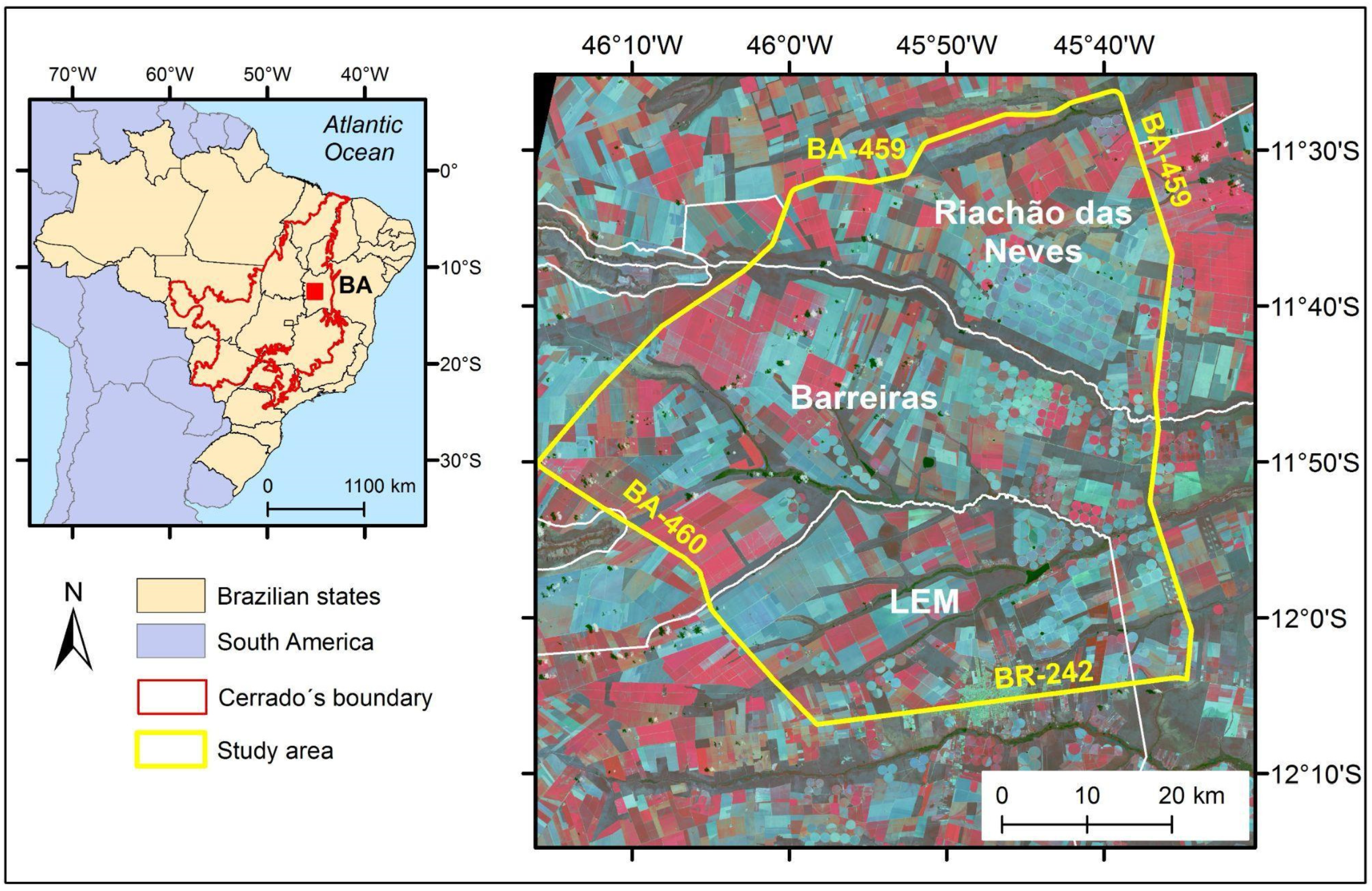
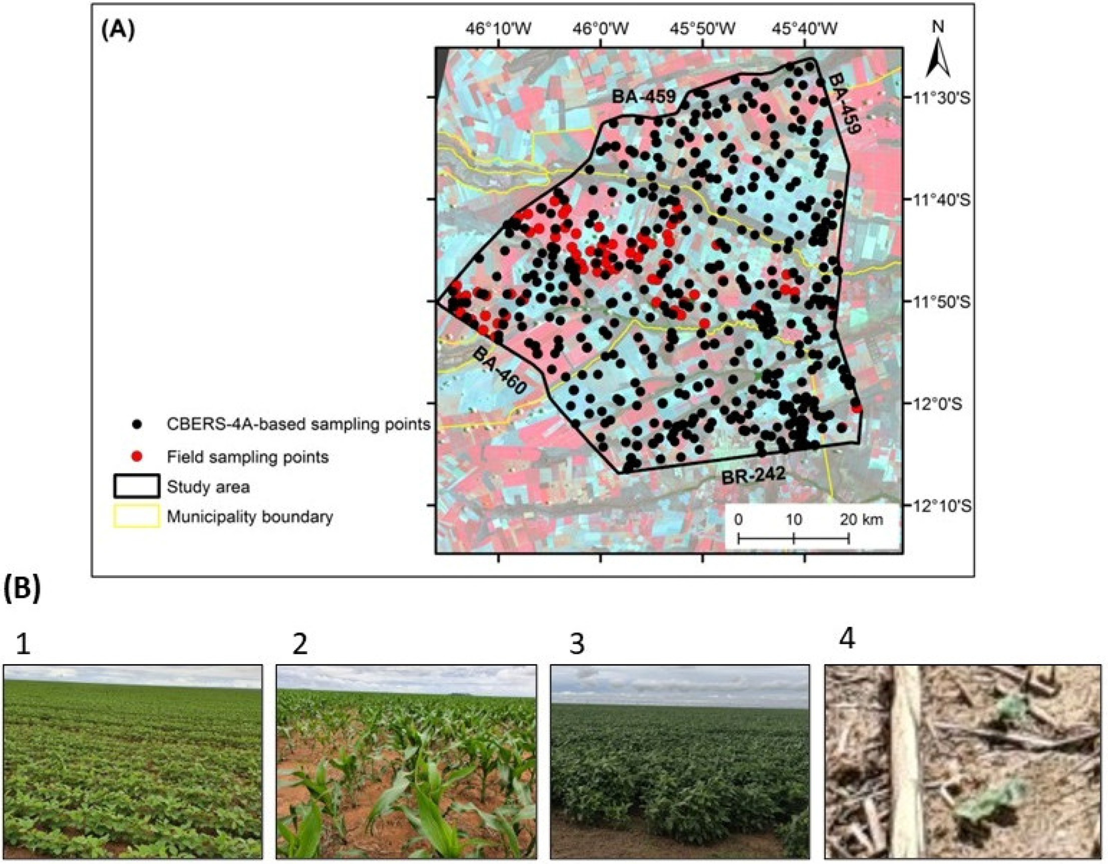
2.1. Study Area
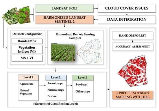
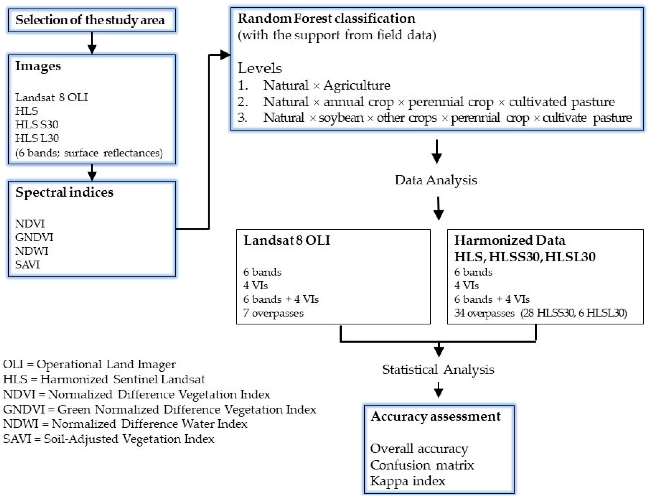
2.2. Methods
2.3. Data Sets
Spectral Vegetation Indices (VIs)
2.4. Hierarchical Classification
Image Classification and Parameterization
2.5. Accuracy Assessment and Statistical Analysis
3. Results
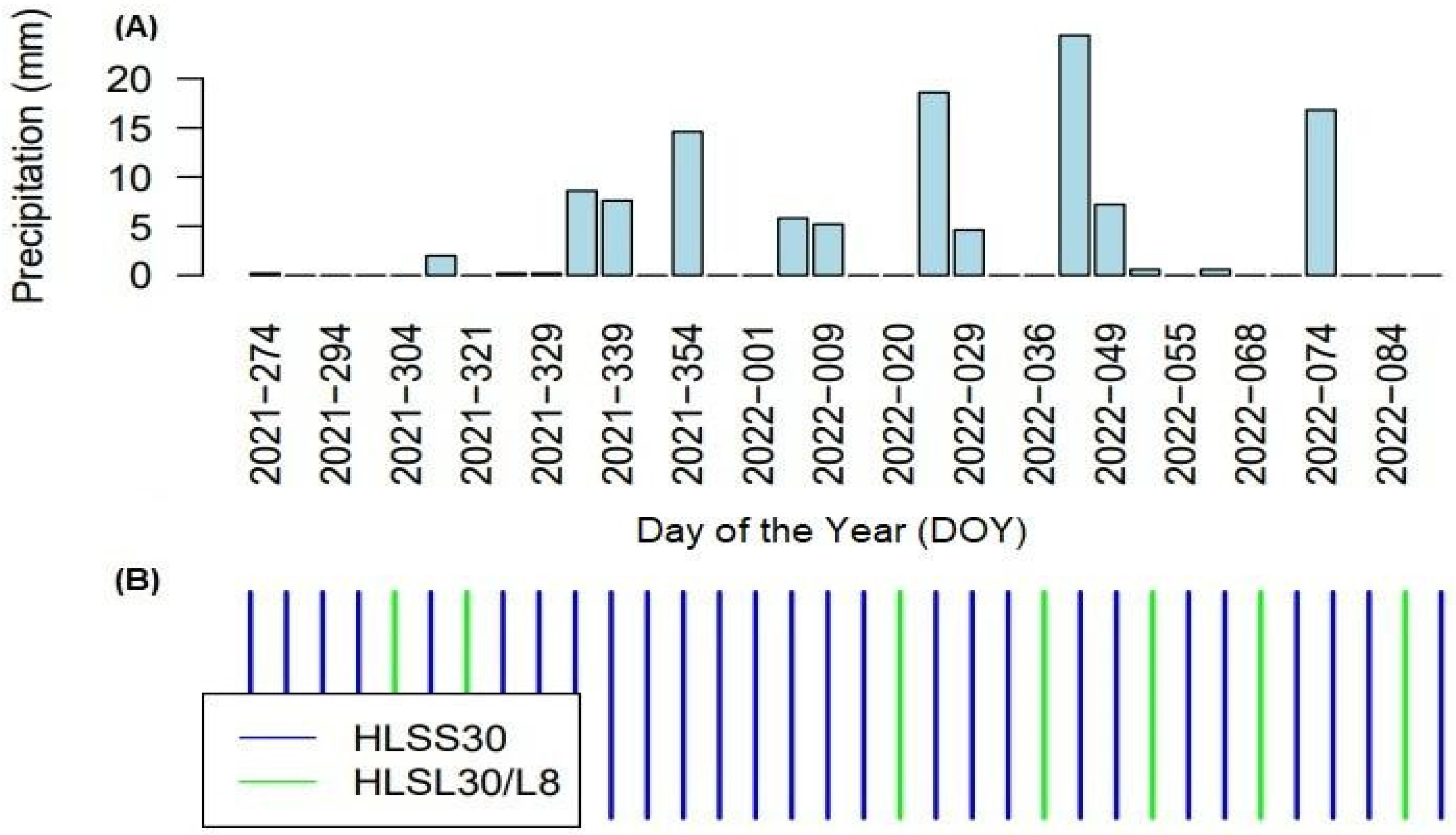
3.1. Influence of Cloud Cover on Satellite Data Availability
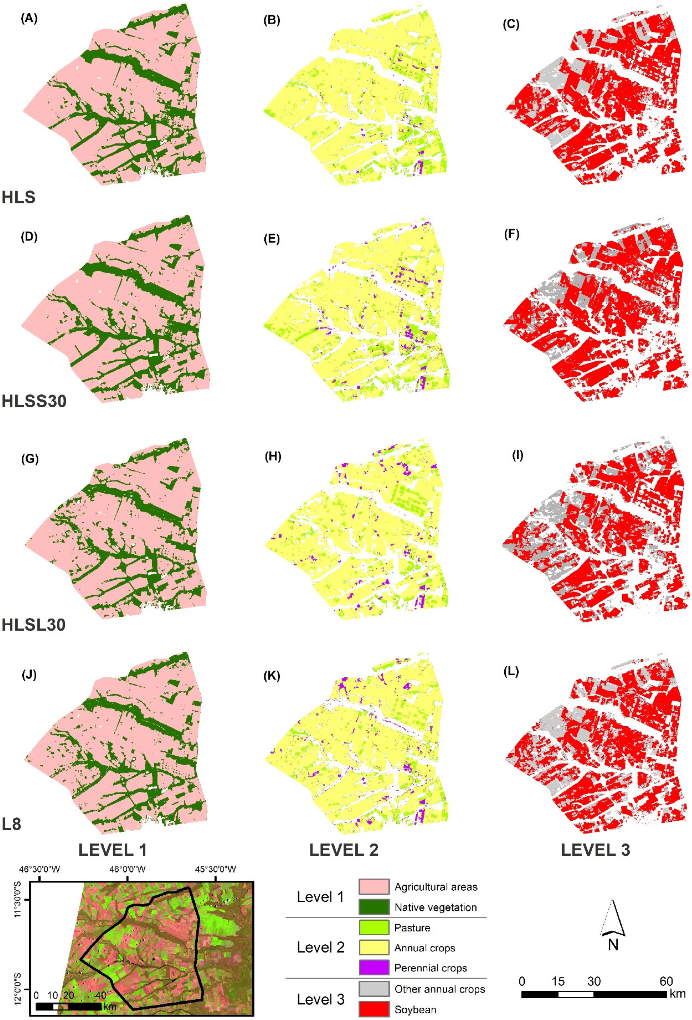
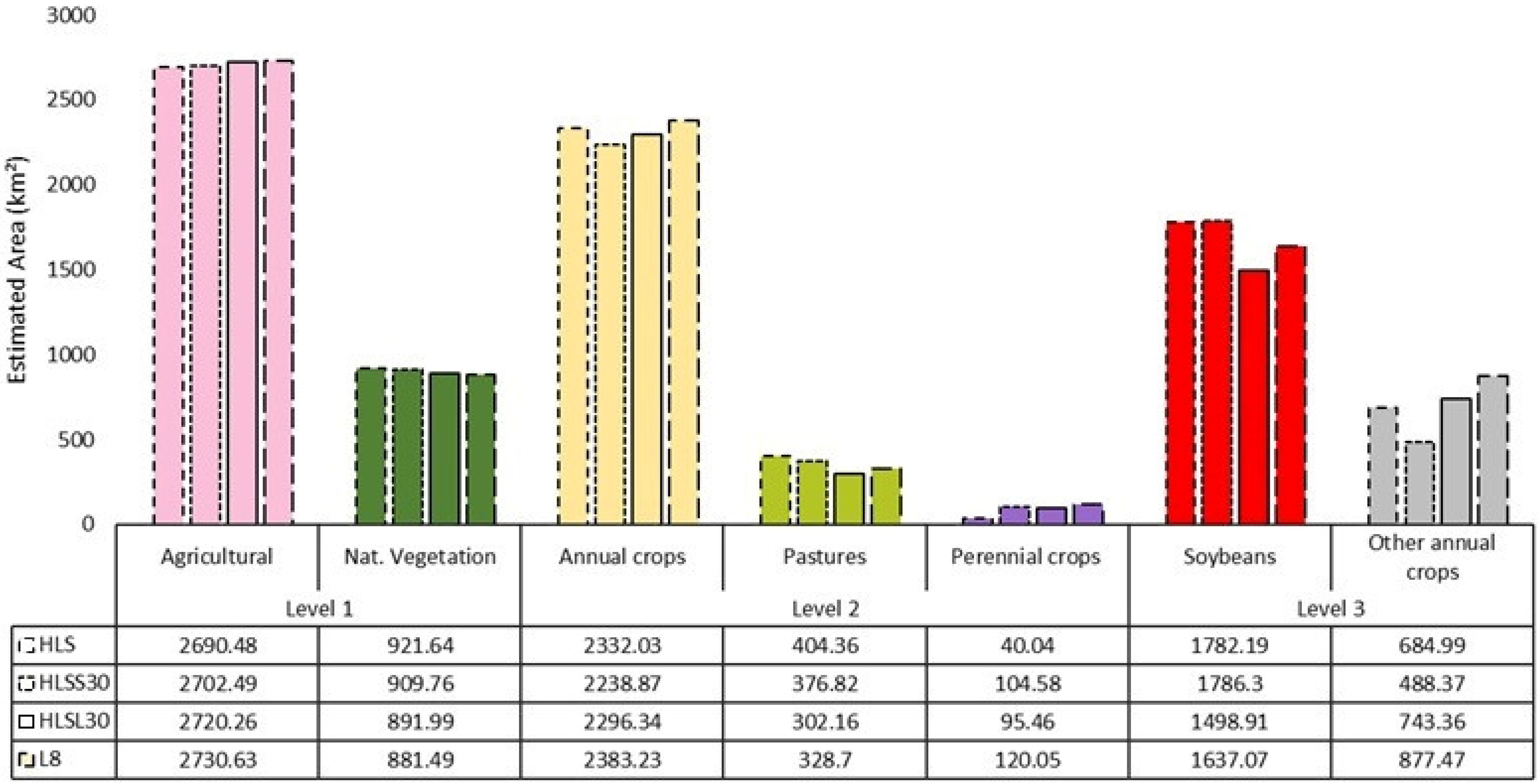
3.2. Classification Results
3.3. Accuracy Assessment and Statistical Analysis
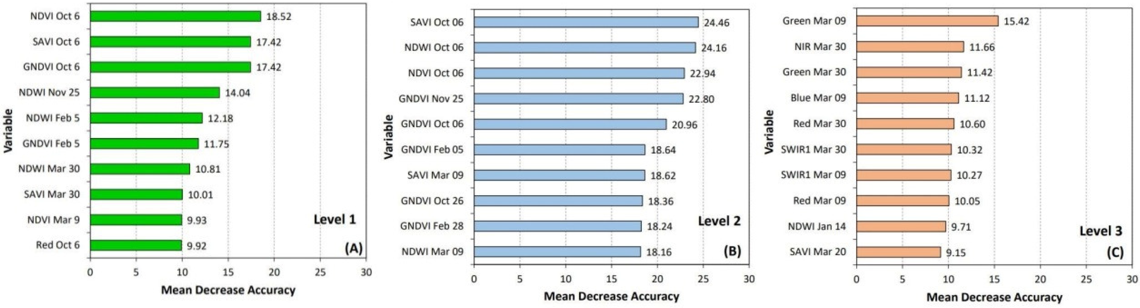
3.4. Variable Importance
4. Discussion
4.1. Cloud Cover Interference on Satellite Image Acquisition
4.2. Impact of Parametrization on the RF Classification Performance
4.3. LULC Mapping Challenges and Variables Importance
4.4. HLS Applications in Agricultural Monitoring
5. Conclusions
Supplementary Materials
Author Contributions
Funding
Data Availability Statement
Conflicts of Interest
References
- Spera, S. Agricultural intensification can preserve the Brazilian Cerrado: Applying lessons from Mato Grosso and Goiás to Brazil’s last agricultural frontier. Trop. Conserv. Sci. 2017, 10, 1–7. [Google Scholar] [CrossRef] [Green Version]
- FAO—Food and Agriculture Organization of the United Nations FAOSTAT—Crops and Livestock Products. Available online: https://https://www.fao.org/faostat/en/#data/QCL (accessed on 10 June 2022).
- Bolfe, É.L.; Jorge, L.A.D.C.; Sanches, I.D.; Luchiari Júnior, A.; da Costa, C.C.; Victoria, D.D.C.; Inamasu, R.Y.; Grego, C.R.; Ferreira, V.R.; Ramirez, A.R. Precision and Digital Agriculture: Adoption of technologies and perception of Brazilian farmers. Agriculture 2020, 10, 653. [Google Scholar] [CrossRef]
- Rada, N. Assessing Brazil’s Cerrado agricultural miracle. Food Policy 2013, 38, 146–155. [Google Scholar] [CrossRef]
- Santana, C.; Souza, G.; Campos, S.; Sanches, I.; Gomes, E.; Sano, E. Dinâmicas agropecuárias e socioeconômicas no Cerrado, de 1975 a 2015. In Dinâmica agrícola no Cerrado: Análises e Projeções; Bolfe, É., Sano, E., Campos, S., Eds.; Embrapa: Brasília, Brazil, 2020; Volume 1, pp. 1–308. [Google Scholar]
- Sano, E.E.; Rodrigues, A.A.; Martins, E.S.; Bettiol, G.M.; Bustamante, M.M.C.; Bezerra, A.S.; Couto, A.F.; Vasconcelos, V.; Schüler, J.; Bolfe, E.L. Cerrado ecoregions: A spatial framework to assess and prioritize Brazilian Savanna environmental diversity for conservation. J. Environ. Manag. 2019, 232, 818–828. [Google Scholar] [CrossRef] [PubMed]
- Pimenta, F.M.; Speroto, A.T.; Costa, M.H.; Dionizio, E.A. Historical changes in land use and suitability for future agriculture expansion in Western Bahia, Brazil. Remote Sens. 2021, 13, 1088. [Google Scholar] [CrossRef]
- Chaves, M.E.D.; Soares, A.R.; Sanches, I.D.; Fronza, J.G. CBERS data cubes for land use and land cover mapping in the Brazilian Cerrado Agricultural Belt. Int. J. Remote Sens. 2021, 42, 8398–8432. [Google Scholar] [CrossRef]
- Rattis, L.; Brando, P.M.; Macedo, M.N.; Spera, S.A.; Castanho, A.D.A.; Marques, E.Q.; Costa, N.Q.; Silverio, D.V.; Coe, M.T. Climatic limit for agriculture in Brazil. Nat. Clim. Chang. 2021, 11, 1098–1104. [Google Scholar] [CrossRef]
- Araújo, M.L.S.; Sano, E.E.; Bolfe, É.L.; Santos, J.R.N.; dos Santos, J.S.; Silva, F.B. Spatiotemporal dynamics of soybean crop in the Matopiba region, Brazil (1990–2015). Land Use Policy. 2019, 80, 57–67. [Google Scholar] [CrossRef]
- Portman, F.T.; Siebert, S.; Döll, P. MIRCA2000—Global monthly irrigated and rainfed crop areas around the year 2000: A new high-resolution data set for agricultural and hydrological modeling. Glob. Biogeochem. Cycles 2010, 24, GB1011. [Google Scholar] [CrossRef]
- Sano, E.E.; Rosa, R.; Brito, J.L.S.; Ferreira, L.G. Land cover mapping of the tropical Savanna region in Brazil. Environ. Monit. Assess. 2010, 166, 113–124. [Google Scholar] [CrossRef]
- Prudente, V.H.R.; Martins, V.S.; Vieira, D.C.; e Silva, N.R.D.F.; Adami, M.; Sanches, I.D. Limitations of cloud cover for optical remote sensing of agricultural areas across South America. Remote Sens. Appl. Soc. Environ. 2020, 20, 100414. [Google Scholar] [CrossRef]
- Luo, Y.; Guan, K.; Peng, J. A generic and fully-automated method to fuse multiple sources of optical satellite data to generate a high-resolution, daily and cloud-/gap-free surface reflectance product. Remote Sens. Environ. 2018, 214, 87–99. [Google Scholar] [CrossRef]
- Gao, F.; Masek, F.; Schwaller, M.; Hall, F. STAIR: On the blending of the Landsat and MODIS surface reflectance: Predicting daily Landsat surface reflectance. IEEE Trans. Geosci. Remote Sens. 2006, 44, 2207–2218. [Google Scholar] [CrossRef]
- Gao, F.; Anderson, M.C.; Zhang, X.; Yang, Z.; Alfieri, J.G.; Kustas, W.P.; Mueller, R.; Johnson, D.M.; Prueger, J.H. Toward mapping crop progress at field scales through fusion of Landsat and MODIS imagery. Remote Sens. Environ. 2017, 188, 9–25. [Google Scholar] [CrossRef] [Green Version]
- Sun, R.; Chen, S.; Su, H.; Mi, C.; Jin, N. The Effect of NDVI time series density derived from spatiotemporal fusion of multisource remote sensing data on crop classification accuracy. ISPRS Int. J. Geo. Inf. 2019, 8, 502. [Google Scholar] [CrossRef] [Green Version]
- Dhillon, M.S.; Dahms, T.; Kübert-Flock, C.; Steffan-Dewenter, I.; Zhang, J.; Ullmann, T. Spatiotemporal fusion modelling using STARFM: Examples of Landsat 8 and Sentinel-2 NDVI in Bavaria. Remote Sens. 2022, 14, 677. [Google Scholar] [CrossRef]
- Zhu, X.; Cai, F.; Tian, J.; Williams, T.K.-A. Spatiotemporal fusion of multisource remote sensing data: Literature survey, Taxonomy, principles, applications, and future directions. Remote Sens. 2018, 10, 527. [Google Scholar] [CrossRef] [Green Version]
- Zhu, X.; Chen, J.; Gao, F.; Chen, X.; Masek, J.G. An enhanced spatial and temporal adaptive reflectance fusion model for complex heterogeneous regions. Remote Sens. Environ. 2010, 114, 2610–2623. [Google Scholar] [CrossRef]
- Hilker, T.; Wulder, M.A.; Coops, N.C.; Linke, J.; McDermid, G.; Masek, J.G.; Gao, F.; White, J.C. A new data fusion model for high spatial- and temporal-resolution mapping of forest disturbance based on Landsat and MODIS. Remote Sens. Environ. 2009, 113, 1613–1627. [Google Scholar] [CrossRef]
- Claverie, M.; Ju, J.; Masek, J.G.; Dungan, J.L.; Vermote, E.F.; Roger, J.-C.; Skakun, S.; Justice, C. The Harmonized Landsat and Sentinel-2 Surface reflectance data set. Remote Sens. Environ. 2018, 219, 145–161. [Google Scholar] [CrossRef]
- Skakun, S.; Vermote, E.; Franch, B.; Roger, J.-C.; Kussul, N.; Ju, J.; Masek, J. Winter wheat yield assessment from Landsat 8 and Sentinel-2 Data: Incorporating surface reflectance, through phenological fitting, into regression yield models. Remote Sens. 2019, 11, 1768. [Google Scholar] [CrossRef] [Green Version]
- Zhang, H.K.; Roy, D.P.; Yan, L.; Li, Z.; Huang, H.; Vermote, E.; Skakun, S.; Roger, J.-C. Characterization of Sentinel-2A and Landsat-8 Top of Atmosphere, surface, and Nadir BRDF adjusted reflectance and NDVI differences. Remote Sens. Environ. 2018, 215, 482–494. [Google Scholar] [CrossRef]
- Franch, B.; Vermote, E.; Skakun, S.; Roger, J.-C.; Masek, J.; Ju, J.; Villaescusa-Nadal, J.; Santamaria-Artigas, A. A method for Landsat and Sentinel 2 (HLS) BRDF normalization. Remote Sens. 2019, 11, 632. [Google Scholar] [CrossRef] [Green Version]
- Torbick, N.; Huang, X.; Ziniti, B.; Johnson, D.; Masek, J.; Reba, M. Fusion of moderate resolution earth observations for operational crop type mapping. Remote Sens. 2018, 10, 1058. [Google Scholar] [CrossRef] [Green Version]
- Hao, P.; Tang, H.; Chen, Z.; Yu, L.; Wu, M. High resolution crop intensity mapping using Harmonized Landsat-8 and Sentinel-2 data. J. Integr. Agric. 2019, 18, 2883–2897. [Google Scholar] [CrossRef]
- Dong, T.; Liu, J.; Qian, B.; He, L.; Liu, J.; Wang, R.; Jing, Q.; Champagne, C.; McNairn, H.; Powers, J.; et al. Estimating crop biomass using leaf area index derived from Landsat 8 and Sentinel-2 data. ISPRS J. Photogramm. Remote Sens. 2020, 168, 236–250. [Google Scholar] [CrossRef]
- Gao, F.; Anderson, M.; Daughtry, C.; Karnieli, A.; Hively, D.; Kustas, W. A within-season approach for detecting early growth stages in corn and soybean using high temporal and spatial resolution imagery. Remote Sens. Environ. 2020, 242, 111752. [Google Scholar] [CrossRef]
- Bolognesi, S.F.; Pasolli, E.; Belfiore, O.; de Michele, C.; D’Urso, G. Harmonized Landsat 8 and Sentinel-2 time Sseries data to detect irrigated areas: An application in southern Italy. Remote Sens. 2020, 12, 1275. [Google Scholar] [CrossRef] [Green Version]
- Griffiths, P.; Nendel, C.; Pickert, J.; Hostert, P. Towards national-scale characterization of grassland use intensity from integrated Sentinel-2 and Landsat time series. Remote Sens. Environ. 2020, 238, 111124. [Google Scholar] [CrossRef]
- Zhou, Q.; Rover, J.; Brown, J.; Worstell, B.; Howard, D.; Wu, Z.; Gallant, A.; Rundquist, B.; Burke, M. Monitoring landscape dynamics in Central U.S. grasslands with Harmonized Landsat-8 and Sentinel-2 time series data. Remote Sens. 2019, 11, 328. [Google Scholar] [CrossRef] [Green Version]
- Pastick, N.J.; Dahal, D.; Wylie, B.K.; Parajuli, S.; Boyte, S.P.; Wu, Z. Characterizing land surface phenology and exotic annual grasses in dryland ecosystems using Landsat and Sentinel-2 Data in harmony. Remote Sens. 2020, 12, 725. [Google Scholar] [CrossRef] [Green Version]
- Bolton, D.K.; Gray, J.M.; Melaas, E.K.; Moon, M.; Eklundh, L.; Friedl, M.A. Continental-scale land surface phenology from Harmonized Landsat 8 and Sentinel-2 imagery. Remote Sens. Environ. 2020, 240, 111685. [Google Scholar] [CrossRef]
- IBGE. Produção Agrícola Municipal. Available online: https://www.ibge.gov.br/estatisticas/economicas/agricultura-e-pecuaria/9117-producao-agricola-municipal-culturas-temporarias-e-permanentes.html?=&t=destaques (accessed on 15 February 2022).
- Alvares, C.A.; Stape, J.L.; Sentelhas, P.C.; Gonçalves, J.L.M.; Sparovek, G. Köppen’s climate classification map for Brazil. Meteorol. Z. 2013, 22, 711–728. [Google Scholar] [CrossRef]
- INMET. Tabelas de Dados das Estações. Available online: https://tempo.inmet.gov.br/TabelaEstacoes/A404 (accessed on 15 February 2022).
- IBGE. Pedologia 1:250,000. Available online: https://www.ibge.gov.br/geociencias/informacoes-ambientais/pedologia/10871-pedologia.html?=&t=acesso-ao-produto (accessed on 20 June 2022).
- USGS. Landsat 8–9 Collection 2 (C2) Level 2 Science Product (L2SP) Guide. Available online: https://d9-wret.s3.us-west-2.amazonaws.com/assets/palladium/production/s3fs-public/media/files/LSDS-1619_Landsat-8-9-C2-L2-ScienceProductGuide-v4.pdf (accessed on 15 February 2022).
- Masek, J.; Ju, J.; Claverie, M.; Skakun, S.; Roger, J.-C.; Vermote, E.; Franch, B.; Yin, Z.; Dungan, J. Harmonized Landsat Sentinel-2 (HLS) Product User Guide—Product Version 2.0. Available online: https://lpdaac.usgs.gov/documents/1326/HLS_User_Guide_V2.pdf (accessed on 15 February 2022).
- Rouse, J.W.; Haas, R.W.; Schell, J.A.; Deering, D.W. Monitoring Vegetation Systems in the Greatplains with ERTS. In Proceedings of the Third ERTS—1 Symposium, NASA Goddard Space Flight Center, Washington, DC, USA, 10–14 December 1974; Volume 1, pp. 309–317. [Google Scholar]
- Gitelson, A.A.; Kaufman, Y.J.; Merzlyak, M.N. Use of a green channel in remote sensing of global vegetation from EOS-MODIS. Remote Sens. Environ. 1996, 58, 289–298. [Google Scholar] [CrossRef]
- Gao, B. NDWI—A Normalized Difference Water Index for remote sensing of vegetation liquid water from space. Remote Sens. Environ. 1996, 58, 257–266. [Google Scholar] [CrossRef]
- Huete, A.R. A Soil-Adjusted Vegetation Index (SAVI). Remote Sens. Environ. 1988, 25, 295–309. [Google Scholar] [CrossRef]
- Huete, A.; Didan, K.; Miura, T.; Rodriguez, E.P.; Gao, X.; Ferreira, L.G. Overview of the radiometric and biophysical performance of the MODIS vegetation indices. Remote Sens. Environ. 2002, 83, 195–213. [Google Scholar] [CrossRef]
- Souza, C.M.; Shimbo, J.Z.; Rosa, M.R.; Parente, L.L.; Alencar, A.A.; Rudorff, B.F.T.; Hasenack, H.; Matsumoto, M.; Ferreira, L.G.; Souza-Filho, P.W.M.; et al. Reconstructing three decades of land use and land cover changes in Brazilian biomes with Landsat archive and Earth Engine. Remote Sens. 2020, 12, 2735. [Google Scholar] [CrossRef]
- IBGE. Áreas Urbanizadas do Brasil: 2015. Available online: https://www.ibge.gov.br/geociencias/cartas-e-mapas/redes-geograficas/15789-areas-urbanizadas.html?=&t=acesso-ao-produto (accessed on 15 February 2022).
- Spinelli-Araújo, L.; Vicente, L.E.; Manzatto, C.V.; Skorupa, L.A.; Victoria, D.D.C.; Soares, A.R. AgroTag: Um sistema de coleta, análise e compartilhamento de dados de campo para qualificação do uso e cobertura das Terras no Brasil. In Proceedings of the XIX Simpósio Brasileiro de Sensoriamento Remoto; INPE—Instituto Nacional de Pesquisas Espaciais, Santos, Brazil, 14–17 April 2019; pp. 451–454. [Google Scholar]
- Congalton, R.G.; Green, K. Assessing the Accuracy of Remotely Sensed Data: Principles and Practices, 3rd ed.; CRC Press: Boca Raton, FL, USA, 2019. [Google Scholar]
- Breiman, L. Random Forests. Mach. Learn. 2001, 45, 5–32. [Google Scholar] [CrossRef] [Green Version]
- Biau, G.; Scornet, E. A Random Forest guided tour. Test 2016, 25, 197–227. [Google Scholar] [CrossRef] [Green Version]
- Fang, P.; Zhang, X.; Wei, P.; Wang, Y.; Zhang, H.; Liu, F.; Zhao, J. The Classification performance and mechanism of machine learning algorithms in winter wheat mapping using Sentinel-2 10 m resolution imagery. Appl. Sci. 2020, 10, 5075. [Google Scholar] [CrossRef]
- Belgiu, M.; Drăguţ, L. Random Forest in remote sensing: A review of applications and future directions. ISPRS J. Photogramm. Remote Sens. 2016, 114, 24–31. [Google Scholar] [CrossRef]
- Arnholt, A.T.; Evans, B. Basic Statistics and Data Analysis (BSDA). Available online: https://cran.r-project.org/web/packages/BSDA/BSDA.pdf (accessed on 25 March 2022).
- MAPA. Zoneamento Agrícola de Risco Climático—Safra 2021/22. Available online: https://indicadores.agricultura.gov.br/zarc/index.htm (accessed on 1 December 2021).
- Dahal, D.; Pastick, N.J.; Boyte, S.P.; Parajuli, S.; Oimoen, M.J.; Megard, L.J. Multi-species inference of exotic annual and native perennial grasses in rangelands of the western United States using Harmonized Landsat and Sentinel-2 data. Remote Sens. 2022, 14, 807. [Google Scholar] [CrossRef]
- Scaramuzza, C.A.M.; Sano, E.E.; Adami, M.; Bolfe, E.L.; Coutinho, A.C.; Esquerdo, J.C.D.M.; Maurano, L.E.P.; Narvaes, I.S.; Oliveira Filho, F.J.B.; Rosa, R.; et al. Land-use and land-cover mapping of the Brazilian Cerrado based mainly on Landsat-8 Satellite images. RBC 2017, 69, 1041–1051. [Google Scholar]
- Nguyen, M.; Baez-Villanueva, O.; Bui, D.; Nguyen, P.; Ribbe, L. Harmonization of Landsat and Sentinel 2 for crop monitoring in drought prone areas: Case studies of Ninh Thuan (Vietnam) and Bekaa (Lebanon). Remote Sens. 2020, 12, 281. [Google Scholar] [CrossRef] [Green Version]
- Ajadi, O.A.; Barr, J.; Liang, S.-Z.; Ferreira, R.; Kumpatla, S.P.; Patel, R.; Swatantran, A. Large-scale crop type and crop area mapping across Brazil using Synthetic Aperture Radar and optical imagery. Int. J. Appl. Earth Obs. Geoinf. 2021, 97, 102294. [Google Scholar] [CrossRef]
- Wang, S.; Azzari, G.; Lobell, D.B. Crop type mapping without field-level labels: Random Forest transfer and unsupervised clustering techniques. Remote Sens. Environ. 2019, 222, 303–317. [Google Scholar] [CrossRef]
- Bolfe, E.L.; Barbedo, J.G.A.; Massruhá, S.M.F.S.; de Souza, K.X.S.; Assad, E.D. Desafios, Tendências e Oportunidades em Agricultura Digital no Brasil. In Agricultura Digital: Pesquisa, Desenvolvimento e Inovação nas Cadeias Produtivas; EMBRAPA: Brasília, Brazil, 2020; Volume 1, pp. 1–406. [Google Scholar]
- Wilkinson, M.D.; Dumontier, M.; Aalbersberg, I.J.; Appleton, G.; Axton, M.; Baak, A.; Blomberg, N.; Boiten, J.-W.; da Silva Santos, L.B.; Bourne, P.E.; et al. The FAIR guiding principles for scientific data management and stewardship. Sci. Data 2016, 3, 160018. [Google Scholar] [CrossRef] [Green Version]
- Zhu, Z.; Wulder, M.A.; Roy, D.P.; Woodcock, C.E.; Hansen, M.C.; Radeloff, V.C.; Healey, S.P.; Schaaf, C.; Hostert, P.; Strobl, P.; et al. Benefits of the free and open Landsat data policy. Remote Sens. Environ. 2019, 224, 382–385. [Google Scholar] [CrossRef]
- Picoli, M.C.A.; Camara, G.; Sanches, I.; Simões, R.; Carvalho, A.; Maciel, A.; Coutinho, A.; Esquerdo, J.; Antunes, J.; Begotti, R.A.; et al. Big Earth Observation time series analysis for monitoring brazilian agriculture. ISPRS J. Photogramm. Remote Sens. 2018, 145, 328–339. [Google Scholar] [CrossRef]
- Oldoni, L.V.; Sanches, I.D.; Picoli, M.C.A.; Covre, R.M.; Fronza, J.G. LEM+ dataset: For agricultural remote sensing applications. Data Br. 2020, 33, 106553. [Google Scholar] [CrossRef] [PubMed]
- Esquerdo, J.C.D.M.; Antunes, J.F.G.; Coutinho, A.C.; Speranza, E.A.; Kondo, A.A.; dos Santos, J.L. SATVeg: A web-based tool for visualization of MODIS vegetation indices in South America. Comput. Electron. Agric. 2020, 175, 105516. [Google Scholar] [CrossRef]
- Wardlow, B.; Egbert, S.; Kastens, J. Analysis of time-series MODIS 250 m vegetation index data for crop classification in the U.S. Central Great Plains. Remote Sens. Environ. 2007, 108, 290–310. [Google Scholar] [CrossRef] [Green Version]
- Martinez, J.A.C.; Rosa, L.E.C.; Feitosa, R.Q.; Sanches, I.D.; Happ, P.N. Fully convolutional recurrent networks for multidate crop recognition from multitemporal image sequences. ISPRS J. Photogramm. Remote Sens. 2021, 171, 188–201. [Google Scholar] [CrossRef]
- Bendini, H.N.; Fonseca, L.M.G.; Schwieder, M.; Körting, T.S.; Rufin, P.; Sanches, I.D.; Leitão, P.J.; Hostert, P. Detailed agricultural land classification in the Brazilian Cerrado based on phenological information from dense satellite image time series. Int. J. Appl. Earth Obs. Geoinf. 2019, 82, 101872. [Google Scholar] [CrossRef]
- Montibeller, B.; Sanches, I.D.; Luiz, A.J.B.; Gonçalves, F.; Aguiar, D.A. Spectral-temporal profile analysis of maize, soybean and sugarcane based on OLI/Landsat-8 data. Braz. J. Agric. 2019, 94, 242–258. [Google Scholar] [CrossRef]
- Epiphanio, R.D.V.; Formaggio, A.R.; Rudorff, B.F.T.; Maeda, E.E.; Luiz, A.J.B. Estimating soybean crop areas using spectral-temporal surfaces derived from MODIS images in Mato Grosso, Brazil. Pesqui. Agropecu. Bras. 2010, 45, 72–80. [Google Scholar] [CrossRef]
- Arvor, D.; Meirelles, M.; Dubreuil, V.; Bégué, A.; Shimabukuro, Y.E. Analyzing the agricultural transition in Mato Grosso, Brazil, using satellite-derived indices. Appl. Geogr. 2012, 32, 702–713. [Google Scholar] [CrossRef] [Green Version]
- Chen, Y.; Lu, D.; Moran, E.; Batistella, M.; Dutra, L.V.; Sanches, I.D.; da Silva, R.F.B.; Huang, J.; Luiz, A.J.B.; de Oliveira, M.A.F. Mapping croplands, cropping patterns, and crop types using MODIS time-series data. Int. J. Appl. Earth Obs. Geoinf. 2018, 69, 133–147. [Google Scholar] [CrossRef]
- Wang, N.; Zhai, Y.; Zhang, L. Automatic cotton mapping using time series of Sentinel-2 images. Remote Sens. 2021, 13, 1355. [Google Scholar] [CrossRef]
- Xun, L.; Zhang, J.; Cao, D.; Yang, S.; Yao, F. A novel cotton mapping index combining Sentinel-1 SAR and Sentinel-2 multispectral imagery. ISPRS J. Photogramm. Remote Sens. 2021, 181, 148–166. [Google Scholar] [CrossRef]
- Xue, J.; Su, B. Significant remote sensing vegetation indices: A review of developments and applications. J. Sens. 2017, 2017, 1–17. [Google Scholar] [CrossRef] [Green Version]
- Vilela, L.; Manjabosco, E.A.; Marchão, R.L.; Guimarães Júnior, R. Integrated Crop-Livestock in Western Bahia State: The Off-Season Cattle Model; (Circular Técnica 37); Embrapa Cerrados: Planaltina, Brazil, 2018. [Google Scholar] [CrossRef]
- Beuchle, R.; Grecchi, R.C.; Shimabukuro, Y.E.; Seliger, R.; Eva, H.D.; Sano, E.; Achard, F. Land cover changes in the brazilian Cerrado and Caatinga biomes from 1990 to 2010 based on a systematic remote sensing sampling approach. Appl. Geogr. 2015, 58, 116–127. [Google Scholar] [CrossRef]
- Müller, H.; Rufin, P.; Griffiths, P.; Barros Siqueira, A.J.; Hostert, P. Mining dense Landsat time series for separating cropland and pasture in a heterogeneous Brazilian Savanna landscape. Remote Sens. Environ. 2015, 156, 490–499. [Google Scholar] [CrossRef] [Green Version]
- Small, C.; Sousa, D. Spatiotemporal characterization of mangrove phenology and disturbance response: The angladesh Sundarban. Remote Sens. 2019, 11, 2063. [Google Scholar] [CrossRef] [Green Version]
- Shen, Y.; Zhang, X.; Yang, Z. Mapping corn and soybean phenometrics at field scales over the United States Corn Belt by fusing time series of Landsat 8 and Sentinel-2 data with VIIRS data. ISPRS J. Photogramm. Remote Sens. 2022, 186, 55–69. [Google Scholar] [CrossRef]
- Gao, F.; Anderson, M.C.; Johnson, D.M.; Seffrin, R.; Wardlow, B.; Suyker, A.; Diao, C.; Browning, D.M. Towards routine mapping of crop emergence within the season using the Harmonized Landsat and Sentinel-2 dataset. Remote Sens. 2021, 13, 5074. [Google Scholar] [CrossRef]
- Nguyen, L.H.; Henebry, G.M. Characterizing land use/land cover using multi-sensor time series from the perspective of land surface phenology. Remote Sens. 2019, 11, 1677. [Google Scholar] [CrossRef] [Green Version]
- Wang, J.; Xiao, X.; Liu, L.; Wu, X.; Qin, Y.; Steiner, J.L.; Dong, J. Mapping sugarcane plantation dynamics in Guangxi, China, by time series Sentinel-1, Sentinel-2 and Landsat images. Remote Sens. Environ. 2020, 247, 111951. [Google Scholar] [CrossRef]
- Xu, F.; Li, Z.; Zhang, S.; Huang, N.; Quan, Z.; Zhang, W.; Liu, X.; Jiang, X.; Pan, J.; Prishchepov, A.V. Mapping winter wheat with combinations of temporally aggregated Sentinel-2 and Landsat-8 data in Shandong Province, China. Remote Sens. 2020, 12, 2065. [Google Scholar] [CrossRef]
- Parreiras, T.C.; Bolfe, E.B.; Sano, S.E.; Victoria, D.C.; Sanches, I.D.; Vicente, L.E. Exploring the Harmonized Landsat and Sentinel-2 (HLS) datacube to map an agricultural landscape in the Brazilian Savanna. Int. Arch. Photogramm. Remote Sens. Spatial Inf. Sci. 2022, 43, 967–973. [Google Scholar] [CrossRef]
- Blickensdörfer, L.; Schwieder, M.; Pflugmacher, D.; Nendel, C.; Erasmi, S.; Hostert, P. Mapping of crop types and crop sequences with combined time series of Sentinel-1, Sentinel-2 and Landsat 8 data for Germany. Remote Sens. Environ. 2022, 269, 112831. [Google Scholar] [CrossRef]
- Liu, L.; Xiao, X.; Qin, Y.; Wang, J.; Xu, X.; Hu, Y.; Qiao, Z. Mapping cropping intensity in China using time series Landsat and Sentinel-2 images and Google Earth Engine. Remote Sens. Environ. 2020, 239, 111624. [Google Scholar] [CrossRef]
- Xue, J.; Anderson, M.C.; Gao, F.; Hain, C.; Yang, Y.; Knipper, K.R.; Kustas, W.P.; Yang, Y. Mapping daily evapotranspiration at field scale using the Harmonized Landsat and Sentinel-2 dataset, with sharpened VIIRS as a Sentinel-2 thermal proxy. Remote Sens. 2021, 13, 3420. [Google Scholar] [CrossRef]
- Xue, J.; Anderson, M.C.; Gao, F.; Hain, C.; Sun, L.; Yang, Y.; Knipper, K.R.; Kustas, W.P.; Torres-Rua, A.; Schull, M. Sharpening ECOSTRESS and VIIRS Land Surface Temperature using Harmonized Landsat-Sentinel surface reflectances. Remote Sens. Environ. 2020, 251, 112055. [Google Scholar] [CrossRef]
- Schwieder, M.; Wesemeyer, M.; Frantz, D.; Pfoch, K.; Erasmi, S.; Pickert, J.; Nendel, C.; Hostert, P. Mapping grassland mowing events across Germany based on combined Sentinel-2 and Landsat 8 time series. Remote Sens. Environ. 2022, 269, 112795. [Google Scholar] [CrossRef]
- Roy, D.P.; Huang, H.; Boschetti, L.; Giglio, L.; Yan, L.; Zhang, H.H.; Li, Z. Landsat-8 and Sentinel-2 burned area mapping—A combined sensor multi-temporal change detection approach. Remote Sens. Environ. 2019, 231, 111254. [Google Scholar] [CrossRef]
- Tulbure, M.G.; Broich, M.; Perin, V.; Gaines, M.; Ju, J.; Stehman, S.; Pavelsky, T.; Masek, J.G.; Yin, S.; Mai, J.; et al. Can we detect more ephemeral floods with higher density Harmonized Landsat Sentinel 2 data compared to Landsat 8 alone? ISPRS J. Photogramm. Remote Sens. 2022, 185, 232–246. [Google Scholar] [CrossRef]
- Lechler, S.; Picoli, M.C.A.; Soares, A.R.; Sanchez, A.; Chaves, M.E.D.; Verstegen, J. Exploring Nasa’s Harmonized Landsat and Sentinel-2 (HLS) dataset to monitor deforestation in the Amazon Rainforest. Int. Arch. Photogramm. Remote Sens. Spat. Inf. Sci. 2020, 43, 705–711. [Google Scholar] [CrossRef]
- Zhang, Y.; Ling, F.; Wang, X.; Foody, G.M.; Boyd, D.S.; Li, X.; Du, Y.; Atkinson, P.M. Tracking small-scale tropical forest disturbances: Fusing the Landsat and Sentinel-2 data record. Remote Sens. Environ. 2021, 261, 112470. [Google Scholar] [CrossRef]
- Chaves, M.E.D.; Picoli, M.C.A.; Sanches, I.D. Recent Applications of Landsat 8/OLI and Sentinel-2/MSI for Land Use and Land Cover Mapping: A Systematic Review. Remote Sens. 2020, 12, 3062. [Google Scholar] [CrossRef]


| Municipality | Cropping Pattern | Crop Type | Harvested Area (ha) |
|---|---|---|---|
| Barreiras | Annual | Soybean | 195,500 |
| Maize | 18,598 | ||
| Cotton | 23,855 | ||
| Others (beans, sorghum, sugarcane) | 16,435 | ||
| Perennial | Coffee, banana (Musa spp.), orange (Citrus sinensis L.), papaya (Carica papaya L.) | 6364 | |
| Luís Eduardo Magalhães | Annual | Soybean | 162,200 |
| Maize | 14,600 | ||
| Cotton | 16,513 | ||
| Others (beans, sorghum, wheat) | 22,268 | ||
| Perennial | Coffee, banana, orange, papaya | 1451 | |
| Riachão das Neves | Annual | Soybean | 116,500 |
| Maize | 12,200 | ||
| Cotton | 32,895 | ||
| Others (beans, sorghum, cassava) | 7973 | ||
| Perennial | Coffee, banana, orange, papaya | 1175 |
| Integer Value | Bit 7 | Bit 6 | Bit 5 | Bit 4 | Bit 3 | Bit 2 | Bit 1 | Bit 0 |
|---|---|---|---|---|---|---|---|---|
| 64 | 0 | 1 | 0 | 0 | 0 | 0 | 0 | 0 |
| 128 | 1 | 0 | 0 | 0 | 0 | 0 | 0 | 0 |
| VIs | Name | Equation | Reference |
|---|---|---|---|
| NDVI | Normalized Difference Vegetation Index | [41] | |
| GNDVI | Normalized Difference NIR/Green NDVI | [42] | |
| NDWI | Normalized Difference Water Index | [43] | |
| SAVI | Soil-Adjusted Vegetation Index * | [44] |
| Level | Parameter | HLS | L8 | HLSS30 | HLSL30 | ||||||||
|---|---|---|---|---|---|---|---|---|---|---|---|---|---|
| MS | VIs | MS + VIs | MS | VIs | MS + VIs | MS | VIs | MS + VIs | MS | VIs | MS + VIs | ||
| 1 | mTry | 10 | 6 | 14 | 18 | 16 | 19 | 13 | 11 | 12 | 6 | 5 | 6 |
| maxnode | 9 | 14 | 8 | 11 | 9 | 7 | 12 | 9 | 9 | 14 | 8 | 6 | |
| nTree | 50 | 250 | 50 | 150 | 50 | 500 | 50 | 100 | 300 | 50 | 150 | 300 | |
| 2 | mTry | 13 | 6 | 14 | 7 | 4 | 13 | 15 | 15 | 11 | 7 | 14 | 5 |
| maxnode | 10 | 12 | 6 | 14 | 12 | 13 | 12 | 9 | 9 | 12 | 8 | 12 | |
| nTree | 50 | 200 | 500 | 250 | 350 | 50 | 100 | 100 | 150 | 450 | 250 | 300 | |
| 3 | mTry | 9 | 6 | 18 | 9 | 5 | 10 | 14 | 11 | 17 | 8 | 5 | 5 |
| maxnode | 6 | 10 | 8 | 5 | 5 | 7 | 6 | 9 | 10 | 13 | 10 | 13 | |
| nTree | 100 | 50 | 400 | 100 | 50 | 50 | 150 | 500 | 200 | 50 | 100 | 200 | |
| Overpass | % Cloud Cover over the Entire Tile | % Data Loss over the Study Area |
|---|---|---|
| 1 November 2021 | 69 | 97 |
| 17 November 2021 | 29 | 29 |
| 20 January 2022 | 6 | 35 |
| 5 February 2022 | 15 | 17 |
| 21 February 2022 | 51 | 93 |
| 9 March 2022 | 4 | 12 |
| 25 March 2022 | 28 | 45 |
| Month | Total of Overpasses | % Cloud Cover * | Data Loss (%) |
|---|---|---|---|
| October | 4 | 36 | 69 |
| November | 6 | 68 | 61 |
| December | 4 | 77 | 87 |
| January | 7 | 67 | 87 |
| February | 7 | 57 | 71 |
| March | 6 | 44 | 64 |
| Sensor/Data | Classifications | Datasets | OA | Kappa |
|---|---|---|---|---|
| Landsat-8 Operational Land Imager OLI (L8) | Level 1 | L8 MS | 0.938 *** | 0.877 |
| L8 VIs | 0.948 *** | 0.896 | ||
| L8 MS + VIs | 0.959 *** | 0.918 | ||
| Level 2 | L8 MS | 0.839 *** | 0.734 | |
| L8 VIs | 0.935 *** | 0.895 | ||
| L8 MS + VIs | 0.903 *** | 0.840 | ||
| Level 3 | L8 MS | 0.782 ns | 0.559 | |
| L8 VIs | 0.696 ns | 0.349 | ||
| L8 MS + VIs | 0.783 ns | 0.559 | ||
| Harmonized Landsat Sentinel-2 (HLS) | Level 1 | HLS MS | 0.917 *** | 0.835 |
| HLS VIs | 0.938 *** | 0.876 | ||
| HLS MS + VIs | 0.959 *** | 0.917 | ||
| Level 2 | HLS MS | 0.839 *** | 0.726 | |
| HLS VIs | 0.935 *** | 0.892 | ||
| HLS MS + VIs | 0.935 *** | 0.892 | ||
| Level 3 | HLS MS | 0.867 ** | 0.721 | |
| HLS VIs | 0.867 ** | 0.704 | ||
| HLS MS + VIs | 0.913 ** | 0.808 | ||
| Sentinel-2 Multi-spectral Instrument Surface Reflectance (HLSS30) | Level 1 | HLSS30 MS | 0.928 *** | 0.855 |
| HLSS30 VIs | 0.948 *** | 0.897 | ||
| HLSS30 MS + VIs | 0.959 *** | 0.917 | ||
| Level 2 | HLSS30 MS | 0.871 *** | 0.788 | |
| HLSS30 VIs | 0.839 *** | 0.746 | ||
| S30 MS + VIs | 0.871 *** | 0.800 | ||
| Level 3 | HLSS30 MS | 0.869 ** | 0.721 | |
| S30 VIs | 0.783 ns | 0.475 | ||
| S30 MS + VIs | 0.869 *** | 0.704 | ||
| Landsat-8 Land Imager Surface Reflectance and TOA Brightness (HLSL30) | Level 1 | HLSL30 MS | 0.897 *** | 0.794 |
| HLSL30 VIs | 0.845 *** | 0.689 | ||
| HLSL30 MS + VIs | 0.856 *** | 0.708 | ||
| Level 2 | HLSL30 MS | 0.742 * | 0.568 | |
| HLSL30 VIs | 0.774 ** | 0.622 | ||
| HLSL30 MS + VIs | 0.774 ** | 0.622 | ||
| Level 3 | HLSL30 MS | 0.696 ns | 0.414 | |
| HLSL30 VIs | 0.739 ns | 0.425 | ||
| HLSL30 MS + VIs | 0.739 ns | 0.485 |
Publisher’s Note: MDPI stays neutral with regard to jurisdictional claims in published maps and institutional affiliations. |
© 2022 by the authors. Licensee MDPI, Basel, Switzerland. This article is an open access article distributed under the terms and conditions of the Creative Commons Attribution (CC BY) license (https://creativecommons.org/licenses/by/4.0/).
Share and Cite
Parreiras, T.C.; Bolfe, É.L.; Chaves, M.E.D.; Sanches, I.D.; Sano, E.E.; Victoria, D.d.C.; Bettiol, G.M.; Vicente, L.E. Hierarchical Classification of Soybean in the Brazilian Savanna Based on Harmonized Landsat Sentinel Data. Remote Sens. 2022, 14, 3736. https://doi.org/10.3390/rs14153736
Parreiras TC, Bolfe ÉL, Chaves MED, Sanches ID, Sano EE, Victoria DdC, Bettiol GM, Vicente LE. Hierarchical Classification of Soybean in the Brazilian Savanna Based on Harmonized Landsat Sentinel Data. Remote Sensing. 2022; 14(15):3736. https://doi.org/10.3390/rs14153736
Chicago/Turabian StyleParreiras, Taya Cristo, Édson Luis Bolfe, Michel Eustáquio Dantas Chaves, Ieda Del’Arco Sanches, Edson Eyji Sano, Daniel de Castro Victoria, Giovana Maranhão Bettiol, and Luiz Eduardo Vicente. 2022. "Hierarchical Classification of Soybean in the Brazilian Savanna Based on Harmonized Landsat Sentinel Data" Remote Sensing 14, no. 15: 3736. https://doi.org/10.3390/rs14153736