Evidence of Instability in Previously-Mapped Landslides as Measured Using GPS, Optical, and SAR Data between 2007 and 2017: A Case Study in the Portuguese Bend Landslide Complex, California


Abstract
:
1. Introduction
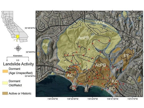
2. Study Area
3. Data and Methodology
3.1. GPS
3.2. COSI-Corr
3.3. PSI
4. Results and Discussion
4.1. GPS and COSI-Corr: Measuring cm- to m-scale Deformation
4.2. PSI to Measure mm-Scale Deformation
4.3. Final Landslide Deformation Map
4.4. Discussion of Multi-Sensor Approaches for Landslide Monitoring
- GPS provides accurate, three-dimensional displacement measurements at a scale ranging from cm to m. In remote sensing studies, GPS data are used as a source of ground-truthing and validation. GPS data are spatially limited as measurements are only available as point sources (e.g., GPS stations).
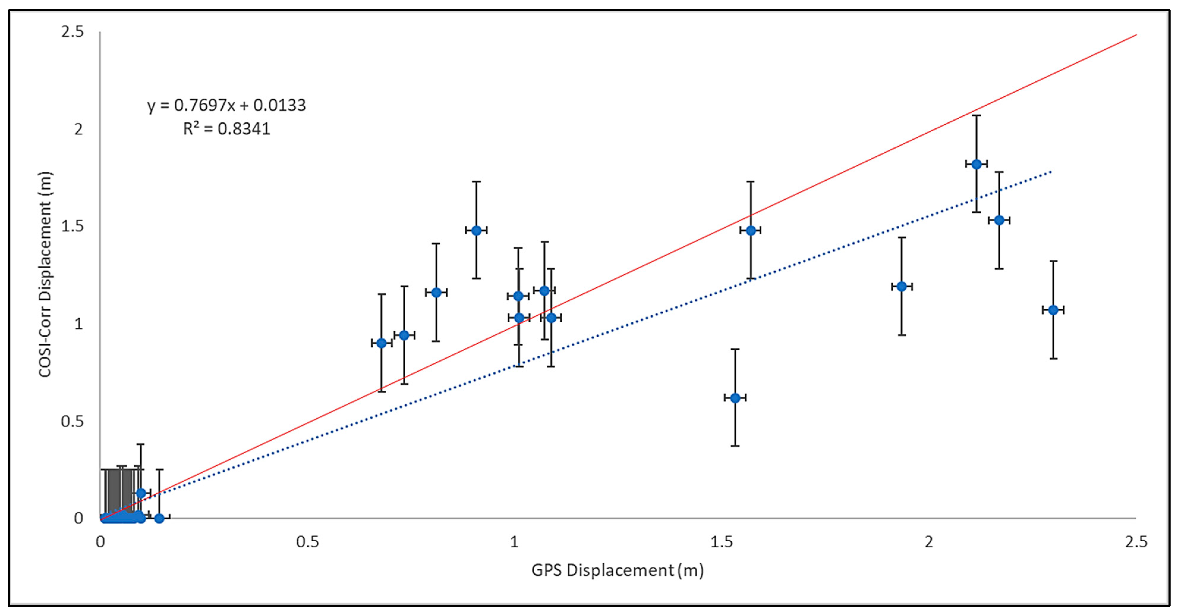
- COSI-Corr processing of optical images allows for two-dimensional displacement measurements at a scale like GPS (cm- to m-scale). COSI-Corr provides a major advantage with respect to spatial coverage, increasing the extent of displacement measurements from point sources (from GPS) to an area equal to the optical image swath. This technique is affected by noise (Figure 6) and cannot accurately measure displacements less than 1/10-pixel size of the optical images.
- PSI processing of SAR images allows for one-dimensional (line-of-sight) displacement measurements at a scale ranging from mm to 1-2 cm. Although PSI cannot measure rapid deformation, it excels at measuring slow-moving deformation (e.g., landslide creep) especially over urban areas, which may be difficult to map in the field.
5. Conclusions
Author Contributions
Funding
Acknowledgments
Conflicts of Interest
Abbreviations
| AC | Abalone Cove (Landslide) |
| AcPB | Active Portuguese Bend (Landslide) |
| AnPB | Ancient Portuguese Bend (Landslide) |
| ASI | Italian Space Agency |
| BC | Beach Club (Landslide) |
| COSI-Corr | Co-registration of Optically Sensed Images and Correlation |
| ESA | European Space Agency |
| FT | Flying Triangle (Landslide) |
| GNSS | Global Navigation Satellite System |
| GPS | Global Positioning System |
| KC | Klondike Canyon (Landslide) |
| P4 | Parcel 4 (Landslide) |
| PS | Persistent Scatterers |
| PSI | Persistent Scatterer Interferometry |
| SAR | Synthetic Aperture Radar |
| VVG | Valley View Graben (Landslide) |
References
- Hungr, O. Dynamics of rapid landslides. In Progress of Landslide Science; Fukuoka, H., Ed.; Springer: Berlin/Heidelberg, Germany, 2007; pp. 47–57. [Google Scholar]
- Dai, F.C.; Lee, C.F.; Ngai, Y.Y. Landslide risk assessment and management: An overview. Eng. Geol. 2002, 64, 65–87. [Google Scholar] [CrossRef]
- Petley, D. Global patterns of loss of life from landslides. Geology 2012, 40, 927–930. [Google Scholar] [CrossRef]
- Ge, Y.G.; Lindell, M.K. County planners’ perceptions of land-use planning tools for environmental hazard mitigation: A survey in the US Pacific states. Environ. Plan. B 2006, 43, 716–736. [Google Scholar] [CrossRef]
- Scolobig, A.; Thompson, M.; Linnerooth-Bayer, J. Compromise not consensus: Designing a participatory process for landslide risk mitigation. Nat. Hazards 2016, 81, 45–68. [Google Scholar] [CrossRef]
- Dou, J.; Yamagishi, H.; Pourghasemi, H.R.; Yunus, A.P.; Song, X.; Xu, Y.; Zhu, Z. An integrated artificial neural network model for the landslide susceptibility assessment of Osado Island, Japan. Nat. Hazards 2015, 78, 1749–1776. [Google Scholar] [CrossRef]
- Gullà, G.; Antronico, L.; Iaquinta, P.; Terranova, O. Susceptibility and triggering scenarios at a regional scale for shallow landslides. Geomorphology 2008, 99, 39–58. [Google Scholar] [CrossRef]
- Hervás, J.; Barredo, J.I.; Rosin, P.L.; Pasuto, A.; Mantovani, F.; Silvano, S. Monitoring landslides from optical remotely sensed imagery: The case history of Tessina landslide, Italy. Geomorphology 2003, 54, 63–75. [Google Scholar] [CrossRef]
- Intrieri, E.; Di Traglia, F.; Del Ventisette, C.; Gigli, G.; Mugnai, F.; Luzi, G.; Casagli, N. Flank instability of Stromboli volcano (Aeolian Islands, Southern Italy): Integration of GB-InSAR and geomorphological observations. Geomorphology 2013, 201, 60–69. [Google Scholar] [CrossRef]
- Intrieri, E.; Gigli, G.; Mugnai, F.; Fanti, R.; Casagli, N. Design and implementation of a landslide early warning system. Eng. Geol. 2012, 147–148, 124–136. [Google Scholar] [CrossRef]
- Jaboyedoff, M.; Oppikofer, T.; Abellán, A.; Derron, M.-H.; Loye, A.; Metzger, R.; Pedrazzini, A. Use of LIDAR in landslide investigations: A review. Nat. Hazards 2012, 61, 5–28. [Google Scholar] [CrossRef]
- Lu, P.; Casagli, N.; Catani, F.; Tofani, V. Persistent Scatterers Interferometry Hotspot and Cluster Analysis (PSI-HCA) for detection of extremely slow-moving landslides. Int. J. Remote Sens. 2012, 33, 466–489. [Google Scholar] [CrossRef]
- McKean, J.; Roering, J. Objective landslide detection and surface morphology mapping using high-resolution airborne laser altimetry. Geomorphology 2004, 57, 331–351. [Google Scholar] [CrossRef]
- Metternicht, G.; Hurni, L.; Gogu, R. Remote sensing of landslides: An analysis of the potential contribution to geo-spatial systems for hazard assessment in mountainous environments. Remote Sens. Environ. 2005, 98, 284–303. [Google Scholar] [CrossRef]
- Michoud, C.; Carrea, D.; Costa, S.; Derron, M.-H.; Jaboyedoff, M.; Delcourt, C.; Maquaire, O.; Letortu, P.; Davidson, R. Landslide detection and monitoring capability of boat-based mobile laser scanning along Dieppe coastal cliffs, Normandy. Landslides 2015, 12, 403–418. [Google Scholar] [CrossRef]
- Ramesh, M.V. Design, development, and deployment of a wireless sensor network for detection of landslides. Ad Hoc Netw. 2014, 13, 2–18. [Google Scholar] [CrossRef]
- Schaefer, L.N.; Lu, Z.; Oommen, T. Dramatic volcanic instability revealed by InSAR. Geology 2015, 43, 743–746. [Google Scholar] [CrossRef] [Green Version]
- Tarantino, C.; Blonda, P.; Pasquariello, G. Remote sensed data for automatic detection of land-use changes due to human activity in support to landslide studies. Nat. Hazards 2007, 41, 245–267. [Google Scholar] [CrossRef]
- Tarolli, P.; Sofia, G.; Dalla Fontana, G. Geomorphic features extraction from high-resolution topography: Landslide crowns and bank erosion. Nat. Hazards 2012, 61, 65–83. [Google Scholar] [CrossRef]
- Thai Pham, B.; Prakash, I.; Dou, J.; Singh, S.K.; Trong Trinh, P.; Trung Tran, H.; Minh Le, T.; Phong Tran, V.; Kim Khoi, D.; Shirzadi, A.; et al. A novel hybrid approach for landslide susceptibility modeling using rotation forest ensemble and different base classifiers. Geocartography Int. 2018, 1–38. [Google Scholar] [CrossRef]
- Young, A.P.; Ashford, S.A. Instability investigation of cantilevered seacliffs. Earth Surf. Process. Landf. 2008, 33, 1661–1677. [Google Scholar] [CrossRef]
- Youssef, A.M.; Maerz, N.H.; Hassan, A.M. Remote sensing applications to geological problems in Egypt: Case study, slope instability investigation, Sharm El-Sheikh/Ras-Nasrani Area, Southern Sinai. Landslides 2009, 6, 353. [Google Scholar] [CrossRef]
- Zhao, C.; Lu, Z.; Zhang, Q.; de la Fuente, J. Large-area landslide detection and monitoring with ALOS/PALSAR imagery data over Northern California and Southern Oregon, USA. Remote Sens. Environ. 2012, 124, 348–359. [Google Scholar] [CrossRef]
- Haydon, W.D. Landslide Inventory Map of the Palos Verdes Peninsula, Los Angeles County; Geologic Information and Publications; California Geological Survey: Sacramento, CA, USA, 2007.
- McMillan, J.R.; Haydon, W.D. Earthquake-Induced Landslide Zones in the Torrance 7.5-Minute Quadrangle, Los Angeles County, California; California Geological Survey Seismic Hazard Zone Report 035, Section 2; California Department of Conservation: Sacramento, CA, USA, 1998; pp. 19–38.
- McMillan, J.R.; Haydon, W.D. Earthquake-Induced Landslides Zones in the San Pedro 7.5-Minute Quadrangle, Los Angeles County, California; California Geological Survey Open File Report 98–24, Section 2; California Department of Conservation: Sacramento, CA, USA, 1998; pp. 15–30.
- McMillan, J.R.; Haydon, W.D. Earthquake-Induced Landslide Zones in the Redondo Beach 7.5-Minute Quadrangle, Los Angeles County; California Geological Survey Seismic Hazard Zone Report 031, Section 2; California Department of Conservation: Sacramento, CA, USA, 1998; pp. 17–35.
- McGee, M. Survey Report of the Portuguese Bend Landslide Monitoring Surveys for the City of Rancho Palos Verdes; McGee Surveying Consulting: Santa Barbara, CA, USA, 2017; 234p. [Google Scholar]
- Cruden, D.M.; Varnes, D.L. Chapter 3: Landslide types and processes. In Landslides: Investigation and Mitigation, Special Report 247; Turner, A.K., Schuster, R.J., Eds.; Transportation Research Board, National Research Council: Washington, DC, USA, 1996; pp. 36–75. [Google Scholar]
- Behling, R.; Roessner, S.; Segl, K.; Kleinschmit, B.; Kaufmann, H. Robust automated image co-registration of optical multi-sensor time series data: Database generation for multi-temporal landslide detection. Remote Sens. 2014, 6, 2572–2600. [Google Scholar] [CrossRef]
- Casagli, N.; Cigna, F.; Bianchini, S.; Hölbling, D.; Füreder, P.; Righini, G.; Del Conte, S.; Friedl, B.; Schneiderbauer, S.; Iasio, C.; et al. Landslide mapping and monitoring by using radar and optical remote sensing: Examples from the EC-FP7 project SAFER. Remote Sens. Soc. Environ. 2016, 4, 92–108. [Google Scholar] [CrossRef] [Green Version]
- Joyce, K.E.; Samsonov, S.V.; Levick, S.R.; Engelbrecht, J.; Belliss, S. Mapping and monitoring geological hazards using optical, LiDAR, and synthetic aperture RADAR image data. Nat. Hazards 2014, 73, 137–163. [Google Scholar] [CrossRef]
- Youssef, A.M.; Sefry, S.A.; Pradhan, B.; Abu Alfadail, E. Analysis on causes of flash flood in Jeddah city (Kingdom of Saudi Arabia) of 2009 and 2011 using multi-sensor remote sensing data and GIS. Geomat. Nat. Hazards Risk 2016, 7, 1018–1042. [Google Scholar] [CrossRef]
- Akbarimehr, M.; Motagh, M.; Haghshenas-Haghighi, M. Slope stability assessment of the Sarcheshmeh landslide, northeast Iran, investigated using InSAR and GPS observations. Remote Sens. 2013, 5, 3681–3700. [Google Scholar] [CrossRef]
- Ao, M.; Wang, C.; Xie, R.; Zhang, X.; Hu, J.; Du, Y.; Li, Z.; Zhu, J.; Dai, W.; Kuang, C. Monitoring the land subsidence with persistent scatterer interferometry in Nansha District, Guangdong, China. Nat. Hazards 2015, 75, 2947–2964. [Google Scholar] [CrossRef]
- Bouali, E.H.; Oommen, T.; Escobar-Wolf, R. Mapping of slow landslides on the Palos Verdes Peninsula using the California landslide inventory and persistent scatterer interferometry. Landslides 2018, 15, 439–452. [Google Scholar] [CrossRef]
- Bovenga, F.; Nitti, D.O.; Fornaro, G.; Radicioni, F.; Stoppini, A.; Brigante, R. Using C/X-band SAR interferometry and GNSS measurements for the Assisi landslide analysis. Int. J. Remote Sens. 2013, 34, 4083–4104. [Google Scholar] [CrossRef]
- Chen, F.; Lin, H.; Yeung, K.; Cheng, S. Detection of slope instability in Hong Kong based on multi-baseline Differential SAR Interferometry using ALOS PALSAR data. GISci. Remote Sens. 2010, 47, 208–220. [Google Scholar] [CrossRef]
- Crosetto, M.; Gili, J.A.; Monserrat, O.; Cuevas-González, M.; Corominas, J.; Serral, D. Interferometric SAR monitoring of the Vallcebre landslide (Spain) using corner reflectors. Nat. Hazards Earth Syst. Sci. 2013, 13, 923–933. [Google Scholar] [CrossRef] [Green Version]
- Gullà, G.; Peduto, D.; Borrelli, L.; Antronico, L.; Fornaro, G. Geometric and kinematic characterization of landslides affecting urban areas: The Lungro case study (Calabria, Southern Italy). Landslides 2017, 14, 171–188. [Google Scholar] [CrossRef]
- Herrera, G.; Gutiérrez, F.; García-Davalillo, J.C.; Guerrero, J.; Notti, D.; Galve, J.P.; Fernández-Merodo, J.A.; Cooksley, G. Multi-sensor advanced DInSAR monitoring of very slow landslides: The Tena Valley case study (Central Spanish Pyrenees). Remote Sens. Environ. 2013, 128, 31–43. [Google Scholar] [CrossRef]
- Komac, M.; Holley, R.; Mahapatra, P.; van der Marel, H.; Bavec, M. Coupling of GPS/GNSS and radar interferometric data for a 3D surface displacement monitoring of landslides. Landslides 2015, 12, 241–257. [Google Scholar] [CrossRef]
- Strozzi, T.; Ambrosi, C.; Raetzo, H. Interpretation of aerial photographs and satellite SAR interferometry for the inventory of landslides. Remote Sens. 2013, 5, 2554–2570. [Google Scholar] [CrossRef]
- Xiao, R.; He, X. GPS and InSAR time series analysis: Deformation monitoring application in a hydraulic engineering resettlement zone, southwest China. Math. Prob. Eng. 2013, 11. [Google Scholar] [CrossRef]
- Fernandez, P.; Whitworth, M. A new technique for the detection of large scale landslides in glacio-lacustrine deposits using image correlation based upon aerial imagery: A case study from the French Alps. Int. J. Appl. Earth Obs. Geoinform. 2016, 52, 1–11. [Google Scholar] [CrossRef] [Green Version]
- Le Bivic, R.; Allemand, P.; Quiquerez, A.; Delacourt, C. Potential and limitation of SPOT-5 ortho-image correlation to investigate the cinematics of landslides: The example of “Mare à Poule d’Eau” (Réunion, France). Remote Sens. 2017, 9, 106. [Google Scholar] [CrossRef]
- Turner, D.; Lucieer, A.; de Jong, S.M. Time series analysis of landslide dynamics using an unmanned aerial vehicle (UAV). Remote Sens. 2015, 7, 1736–1757. [Google Scholar] [CrossRef]
- Bianchini, S.; Cigna, F.; Del Ventisette, C.; Moretti, S.; Casagli, N. Monitoring landslide-induced displacements with TerraSAR-X Persistent Scatterer Interferometry (PSI): Gimigliano case study in Calabria Region (Italy). Int. J. Geosci. 2013, 4, 1467–1482. [Google Scholar] [CrossRef]
- Bianchini, S.; Cigna, F.; Righini, G.; Proietti, C.; Casagli, N. Landslide HotSpot Mapping by means of Persistent Scatterer Interferometry. Environ. Earth Sci. 2012, 67, 1155–1172. [Google Scholar] [CrossRef]
- Del Ventisette, C.; Righini, G.; Moretti, S.; Casagli, N. Multitemporal landslides inventory map updating using spaceborne SAR analysis. Int. J. Appl. Earth Obs. Geoinform. 2014, 30, 238–246. [Google Scholar] [CrossRef] [Green Version]
- Hölbling, D.; Füreder, P.; Antolini, F.; Cigna, F.; Casagli, N.; Lang, S. A semi-automated object-based approach for landslide detection validated by Persistent Scatterer Interferometry measures and landslide inventories. Remote Sens. 2012, 4, 1310–1336. [Google Scholar] [CrossRef]
- Piacentini, D.; Devoto, S.; Mantovani, M.; Pasuto, A.; Prampolini, M.; Soldati, M. Landslide susceptibility modeling assisted by Persistent Scatterer Interferometry (PSI): An example from the northwestern coast of Malta. Nat. Hazards 2015, 78, 681–697. [Google Scholar] [CrossRef]
- Tofani, V.; Raspini, F.; Catani, F.; Casagli, N. Persistent Scatterer Interferometry (PSI) technique for landslide characterization and monitoring. Remote Sens. 2013, 5, 1045–1065. [Google Scholar] [CrossRef]
- Delacourt, C.; Allemand, P.; Casson, B.; Vadon, H. Velocity field of the “La Clapière” landslide measured by the correlation of aerial and QuickBird satellite images. Geophys. Res. Lett. 2004, 31, L15619. [Google Scholar] [CrossRef]
- Laribi, A.; Walstra, J.; Ougrine, M.; Seridi, A.; Dechemi, N. Use of digital photogrammetry for the study of unstable slopes in urban areas: Case study of the El Biar landslide, Algiers. Eng. Geol. 2015, 187, 73–83. [Google Scholar] [CrossRef]
- Tung, S.-H.; Weng, M.-C.; Shih, M.-H. Measuring the in situ deformation of retaining walls by the digital image correlation method. Eng. Geol. 2013, 166, 116–126. [Google Scholar] [CrossRef]
- Ferretti, A.; Prati, C.; Rocca, F. Nonlinear subsidence rate estimation using permanent scatterers in differential SAR interferometry. IEEE Trans. Geosci. Remote 2000, 38, 2202–2212. [Google Scholar] [CrossRef]
- Ferretti, A.; Prati, C.; Rocca, F. Permanent scatterers in SAR interferometry. IEEE Trans. Geosci. Remote 2001, 39, 8–20. [Google Scholar] [CrossRef] [Green Version]
- Crosetto, M.; Monserrat, O.; Cuevas-González, M.; Devanthéry, N.; Crippa, B. Persistent Scatterer Interferometry: A review. ISPRS J. Photogramm. Remote Sens. 2016, 115, 78–89. [Google Scholar] [CrossRef] [Green Version]
- Varnes, D.J. Slope movement types and processes. In Landslides: Analysis and Control., Special Report 176; Schuster, R.L., Krizek, R.J., Eds.; Transportation Research Board, National Research Council: Washington, DC, USA, 1978; pp. 11–33. [Google Scholar]
- Wieczorek, G.F. Preparing a detailed landslide-inventory map for hazard evaluation and reduction. B Assoc. Eng. Geol. 1984, 21, 337–342. [Google Scholar] [CrossRef]
- Keaton, J.R.; DeGraff, J.V. Chapter 9: Surface observation and geologic mapping. In Landslides: Investigation and Mitigation, Special Report 247; Turner, A.K., Schuster, R.J., Eds.; Transportation Research Board, National Research Council: Washington, DC, USA, 1996; pp. 178–230. [Google Scholar]
- Merriam, R. Portuguese Bend landslide, Palos Verdes Hills, California. J. Geol. 1960, 68, 140–153. [Google Scholar] [CrossRef]
- Woodring, W.P.; Bramlette, M.N.; Kew, W.S.W. Geology and Paleontology of Palos Verdes Hills; U.S. Geological Survey, Professional Paper 207; United States Department of the Interior: Washington, DC, USA, 1946; 145p.
- Calabro, M.D.; Schmidt, D.A.; Roering, J.J. An examination of seasonal deformation at the Portuguese Bend landslide, Southern California, using radar interferometry. J. Geophys. Res. 2010, 115, 10. [Google Scholar] [CrossRef]
- Ehlig, P.L.; Bean, R.T. Dewatering of the Abalone Cove landslide, Rancho Palos Verdes, Los Angeles County, CA. In Volume and Guidebook: Landslides and Landslide Abatement, Geological Society of America, Palos Verdes Peninsula, Southern California; Cooper, J.D., Ed.; Geological Society of America Cordilleran Section: Anaheim, CA, USA, 1982; pp. 67–79. [Google Scholar]
- Kayen, R.E.; Lee, H.J.; Hein, J.R. Influence of the Portuguese Bend landslide on the character of the effluent-affected sediment deposit, Palos Verdes margin, Southern California. Cont. Shelf Res. 2002, 22, 911–922. [Google Scholar] [CrossRef]
- Ehlig, P.L. Evolution, mechanics and mitigation of the Portuguese Bend landslide, Palos Verdes Peninsula, CA. In Engineering Geology Practice in Southern California; Pipkin, B.W., Proctor, R.J., Eds.; Special Publication No. 4; Associations of Engineering Geology: Redwood City, CA, USA, 1992. [Google Scholar]
- Proffer, K.A. Ground water in the Abalone Cove landslide, Palos Verdes Peninsula, southern California. In Landslides/Landslide Mitigation; Slosson, J.E., Keene, A.G., Johnson, J.A., Eds.; Geological Society of America: Boulder, CO, USA, 1992; pp. 69–82. [Google Scholar]
- City of Rancho Palos Verdes. Landslide Workshop. 2012. Available online: http://www.rpvca.gov/documentcenter/view/5564 (accessed on 7 March 2019).
- Osier, V. Rancho Palos Verdes Mulling Long-Term Fix for Portuguese Bend Landslide. Daily Breeze. 27 January 2018. Available online: https://www.dailybreeze.com/2018/01/27/rancho-palos-verdes-mulling-long-term-fix-for-portuguese-bend-landslide/ (accessed on 1 March 2019).
- Los Angeles Regional Imagery Acquisition Consortium (LAR-IAC). 10-foot Digital Elevation Model (DEM)–LAR-IAC–Public Domain. 2006. Available online: https://egis3.lacounty.gov/dataportal/2011/01/26/2006-10-foot-digital-elevation-model-dem-public-domain/ (accessed on 1 March 2019).
- Leprince, S.; Ayoub, F.; Lin, J.; Avouac, J.-P.; Muse, P.; Barbot, S. COSI-Corr: Measuring Ground Deformation Using Optical Satellite and Aerial Images. 2004. Available online: http://www.tectonics.caltech.edu/slip_history/spot_coseis/index.html (accessed on 1 March 2019).
- Leprince, S.; Barbot, S.; Ayoub, F.; Avouac, J.-P. Automatic, precise, ortho-rectification and co-registration for satellite image correlation: Application to seismotectonics. IEEE Trans. Geosci. Remote 2007, 45, 1529–1558. [Google Scholar] [CrossRef]
- Ayoub, F.; Leprince, S.; Avouac, J. User’s Guide to COSI-CORR: Co-Registration of Optically Sensed Images and Correlation. California Institute of Technology, 2017. Available online: http://www.tectonics.caltech.edu/slip_history/spot_coseis/pdf_files/CosiCorr-Guide2017.pdf (accessed on 30 March 2019).
- Bridges, N.T.; Ayoub, F.; Avouac, J.-P.; Leprince, S.; Lucas, A.; Mattson, S. Earth-like sand fluxes on Mars. Nature 2012, 485, 339–342. [Google Scholar] [CrossRef] [Green Version]
- Lucieer, A.; de Jong, S.M.; Turner, D. Mapping landslide displacements using Structure from Motion (SfM) and image correlation of multi-temporal UAV photography. Prog. Phys. Geog. 2014, 38, 97–116. [Google Scholar] [CrossRef]
- Necsoiu, M.; Leprince, S.; Hooper, D.M.; Dinwiddie, C.L.; McGinnis, R.N.; Walter, G.R. Monitoring migration rates of an active subarctic dune field using optical imagery. Remote Sens. Environ. 2009, 113, 2441–2447. [Google Scholar] [CrossRef]
- Vermeesch, P.; Drake, N. Remotely sensed dune celerity and sand flux measurements of the world’s fastest barchans (Bodélé, Chad). Geophys. Res. Lett. 2008, 35, L24404. [Google Scholar] [CrossRef]
- Leprince, S. COSI-Corr–Brief Description of COSI-Corr–Introduction; The COSI-Corr Project Discussion Group. 2008. Available online: http://tecto.gps.caltech.edu/forum/viewtopic.php?id=2 (accessed on 30 March 2019).
- Bayer, B.; Simoni, A.; Schmidt, D.; Bertello, L. Using advanced InSAR techniques to monitor landslide deformations induced by tunneling in the Northern Apennines, Italy. Eng. Geol. 2017, 226, 20–32. [Google Scholar] [CrossRef]
- Béjar-Pizarro, M.; Notti, D.; Mateos, R.M.; Ezquerro, P.; Centolanza, G.; Herrera, G.; Bru, G.; Sanabria, M.; Solari, L.; Duro, J.; et al. Mapping vulnerable urban areas affected by slow-moving landslides using Sentinel-1 InSAR data. Remote Sens. 2017, 9, 876. [Google Scholar] [CrossRef]
- Bianchini, S.; Ciampalini, A.; Raspini, F.; Bardi, F.; Di Traglia, F.; Moretti, S.; Casagli, N. Multi-temporal evaluation of landslide movements and impacts on buildings in San Fratello (Italy) by means of C-band and X-band PSI data. Pure Appl. Geophys. 2015, 172, 3043–3065. [Google Scholar] [CrossRef]
- Bianchini, S.; Solari, L.; Casagli, N. A GIS-based procedure for landslide intensity evaluation and specific risk analysis supported by Persistent Scatterers Interferometry (PSI). Remote Sens. 2017, 9, 1093. [Google Scholar] [CrossRef]
- Carlà, T.; Raspini, F.; Intrieri, E.; Casagli, N. A simple method to help determine landslide susceptibility from spaceborne InSAR data: The Montescaglioso case study. Environ. Earth Sci. 2016, 75, 1492. [Google Scholar] [CrossRef]
- Ciampalini, A.; Raspini, F.; Lagomarsino, D.; Catani, F.; Casagli, N. Landslide susceptibility map refinement using PSInSAR data. Remote Sens. Environ. 2016, 184, 302–315. [Google Scholar] [CrossRef] [Green Version]
- Oliveira, S.C.; Zêzere, J.L.; Catalão, J.; Nico, G. The contribution of PSInSAR interferometry to landslide hazard in weak rock-dominated areas. Landslides 2015, 12, 703–719. [Google Scholar] [CrossRef]
- Rosi, A.; Tofani, V.; Tanteri, L.; Tacconi Stefanelli, C.; Agostini, A.; Catani, F.; Casagli, N. The new landslide inventory of Tuscany (Italy) updated with PS-InSAR: Geomorphological features and landslide distribution. Landslides 2018, 15, 5–19. [Google Scholar] [CrossRef]
- Sara, F.; Silvia, B.; Sandro, M. Landslide inventory updating by means of Persistent Scatterer Interferometry (PSI): The Setta basin (Italy) case study. Geomat. Nat. Hazards Risk 2015, 6, 419–438. [Google Scholar] [CrossRef]
- Sun, Q.; Zhang, L.; Ding, X.L.; Hu, J.; Li, Z.W.; Zhu, J.J. Slope deformation prior to Zhouqu, China landslide from InSAR time series analysis. Remote Sens. Environ. 2015, 156, 45–57. [Google Scholar] [CrossRef]
- Xue, Y.T.; Meng, X.M.; Li, K.; Chen, G. Loess Slope Instability Assessment Based on PS-InSAR Detected and Spatial Analysis in Lanzhou Region, China. Adv. Mat. Res. 2015, 1065–1069, 2342–2352. [Google Scholar] [CrossRef]
- Italian Space Agency. COSMO-SkyMed SAR Products Handbook, Rev. 2; Italian Space Agency: Rome, Italy, 2009; 105p. [Google Scholar]
- Sarmap. SARscape v. 5.2 Software; Sarmap: Caslano, Switzerland, 2017. [Google Scholar]
- Schlögel, R.; Doubre, C.; Malet, J.-P.; Masson, F. Landslide deformation monitoring with ALOS/PALSAR imagery: A D-InSAR geomorphological interpretation method. Geomorphology 2015, 231, 314–330. [Google Scholar] [CrossRef]
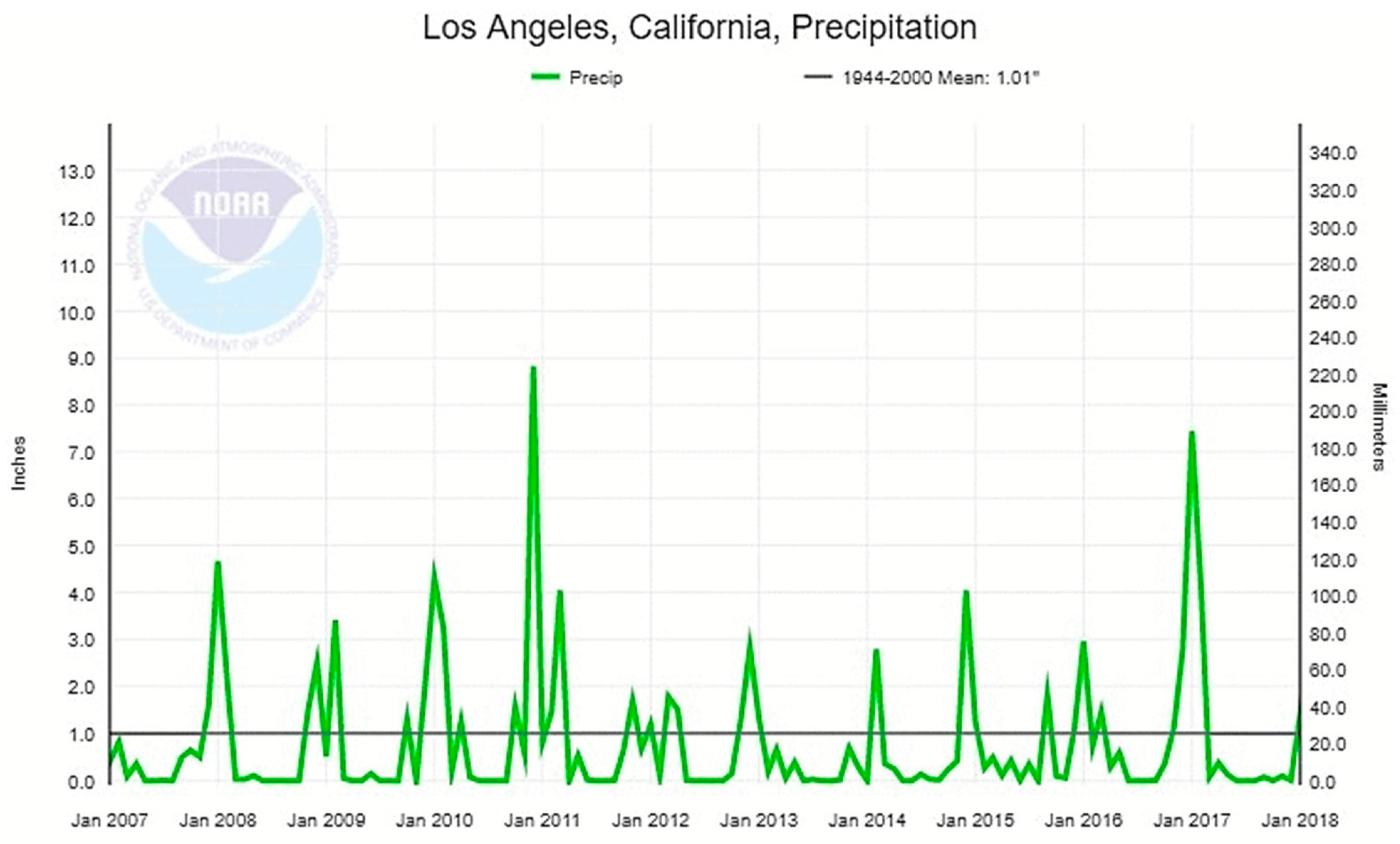
- National Oceanic and Atmospheric Administration (NOAA). Climate at a Glance. 2018. Available online: https://www.ncdc.noaa.gov/cag/city/time-series/USW00023174/pcp/all/6/2007-2018?base_prd=true&firstbaseyear=1944&lastbaseyear=2000 (accessed on 1 March 2019).
- Ehlig, P.L. The Palos Verdes Peninsula: Its physiography, land use and geologic setting. In Volume and Guidebook: Landslides and Landslide Abatement, Geological Society of America, Palos Verdes Peninsula, Southern California; Cooper, J.D., Ed.; Geological Society of America Cordilleran Section: Anaheim, CA, USA, 1982; pp. 3–6. [Google Scholar]


| PSI | COSI-Corr | GPS | |
|---|---|---|---|
| Spatial Distribution of Data Points | Unknown until processing complete | Gridded across spatial extent of input imagery | Installed; must be placed in areas where not disturbed by external factors |
| Temporal Distribution of Data | Spans acquisition period of sensor | Spans acquisition period of sensor | Spans acquisition period post-installation |
| Range of Measurable Deformation Rates | < 2.5 cm/year (threshold changes based on data quality, number of images, and radar wavelength) | cm/year to m/year | cm/year to m/year |
| Direction(s) of Measurements | 1-dimensional, sensor line-of-sight | 2-dimensional, horizontal (north-south and east-west) | 3-dimensional, horizontal and vertical |
| Accuracy | 1 mm/year | 5–10 cm/year | 1–2 cm/year |
| Sources of Noise | Ionospheric effects, snow cover, precipitation, changes in dielectric properties of materials, vegetation, systematic noise | Cloud cover, snow cover, vegetation, drastic changes in ground surface (e.g., construction), systematic noise | Rapid ground deformation (destruction of monuments), external factors (e.g., humans and animals) |
| Measurements Unavailable (Decorrelation) or Unreliable | Dense vegetation, topographic shadow zones, areas with rapid ground deformation | Areas beneath clouds, dense vegetation, topographic shadow zones | If impacted by sources of noise listed above |
| Validation | GPS and other ground-truthing methods | GPS and other ground-truthing methods | Other ground-truthing methods (e.g., surveys) |
| Landslide | Type | Thickness (ft, m) | Activity | Movement Direction (azimuth) | Interpretation Confidence Level |
|---|---|---|---|---|---|
| AnPB | Rock Slide | > 50, > 15.24 | Dormant Old/Relict | 180 | Definite |
| AcPB | Rock Slide | > 50, > 15.24 | Active/Historic | 180 | Definite |
| VVG | Rock Slide | > 50, > 15.24 | Dormant Old/Relict | 180 | Definite |
| P4 | Rock Slide | 10–50, 3.05–15.24 | Dormant Old/Relict | 180 | Definite |
| AC | Rock Slide | > 50, > 15.24 | Active/Historic | 220 | Definite |
| KC | Rock Slide | > 50, > 15.24 | Active/Historic | 220 | Definite |
| BC | Rock Slide | > 50, > 15.24 | Active/Historic | 220 | Definite |
| FT | Rock Slide | > 50, > 15.24 | Active/Historic | 230 | Definite |
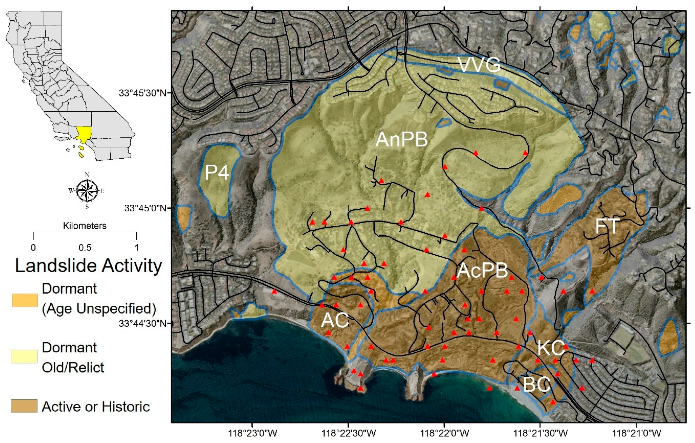
| Year(s) | Measured Deformation | Data Source | Location of Deformation within Landslide Complex | Complementary Figure(s) | |
|---|---|---|---|---|---|
| 2007–2008 | > 1.5 m | GPS | Western and central regions of AcPB and FT | 2A | |
| 1 m–1.5 m | GPS | Southeast region of AnPB and north/northwest regions of AcPB | 2A | ||
| Relatively Stable | GPS | KC and BC | 2A | ||
| 2009 | 1 m–1.5 m | GPS | AcPB deformation decreases slightly (compared to 2007–2008) | 2B | |
| ~1 m | GPS | Eastern toe of FT | 2B | ||
| Relatively Stable | GPS | AnPB and AC (more stable than 2007–2008); KC and BC | 2B | ||
| 2010 | > 1.5 m | GPS | Central region of AcPB remains most active with an increase in deformation since 2009 | 2C | |
| ~1 m | GPS | Eastern toe of FT | 2C | ||
| Relatively Stable | GPS | AnPB, AC, KC, and BC | 2C | ||
| 2011 | > 1 m | GPS | Western and central AcPB, AC, and FT | 2D | |
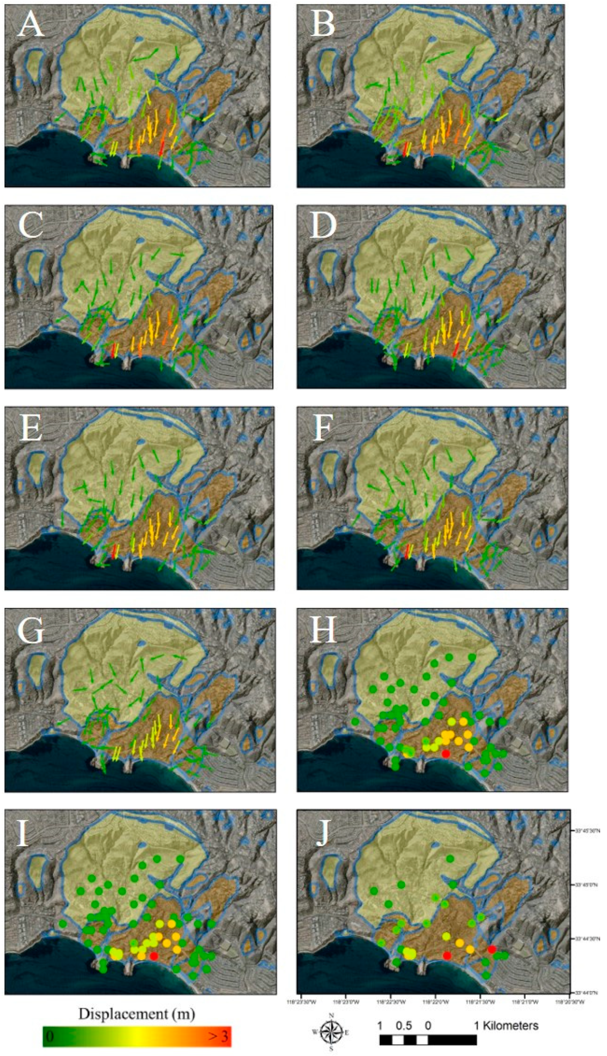
| > 1 m | COSI-Corr | February to May | Widespread instability, including areas not mapped as landslides | 3A | |
| Relatively Stable | COSI-Corr | May to December | Little significant deformation outside landslide complex; none within complex | 3B | |
| 2012 | > 1 m | GPS, COSI-Corr | Activity throughout AcPB | 2E, 3C | |
| ~1 m | GPS | Eastern toe of FT | 2E | ||
| Relatively Stable | GPS, COSI-Corr | AnPB, AC, KC, and BC | 2E, 3C | ||
| 2013 | 3–4 m | COSI-Corr | P4 is most active landslide, with displacement peaking at ~4 m (September) before decreasing to ~3 m | 3D, 3E | |
| > 1.5 m | GPS, COSI-Corr | AcPB remains active, mostly vertical displacement since COSI-Corr does not capture any deformation during this time | 2F, 3D, 3E | ||
| Relatively Stable | GPS, COSI-Corr | AnPB, AC, KC, and BC | 2F, 3D, 3E | ||
| 2014-2015 | 0.5 m–3 m | GPS, COSI-Corr | AcPB remains active, mostly vertical displacement until September 2015 when COSI-Corr measures horizontal displacement ranging from 0.5 m (landslide body) to 3 m (landslide head); | 2G, 2H, 3G | |
| Relatively Stable to ~0.5 m | GPS, COSI-Corr | All landslides adjacent to AcPB stable until September 2015 when COSI-Corr measures ~0.5 m displacement in AnPB | 2G, 2H, 3G | ||
| 2016 | > 3 m | GPS | GPS stations within AcPB measure displacement > 3 m at two locations | 2I | |
| Relatively Stable | GPS | AnPB, AC, KC, and BC | 2I | ||
| 2017 | > 3 m | GPS | GPS stations within AcPB measure displacement > 3 m at two locations | 2J | |
| ~1 m | GPS | Toe of AC | 2J | ||
| Relatively Stable | GPS | AnPB and FT | 2J | ||
| Line of Best Fit Slope | Line of Best Fit Intercept | R2 Value | GPS Error Bars | COSI-Corr Error Bars |
|---|---|---|---|---|
| 0.77 | 0.0133 | 0.8341 | +/- 0.05 m | +/- 0.25 m |
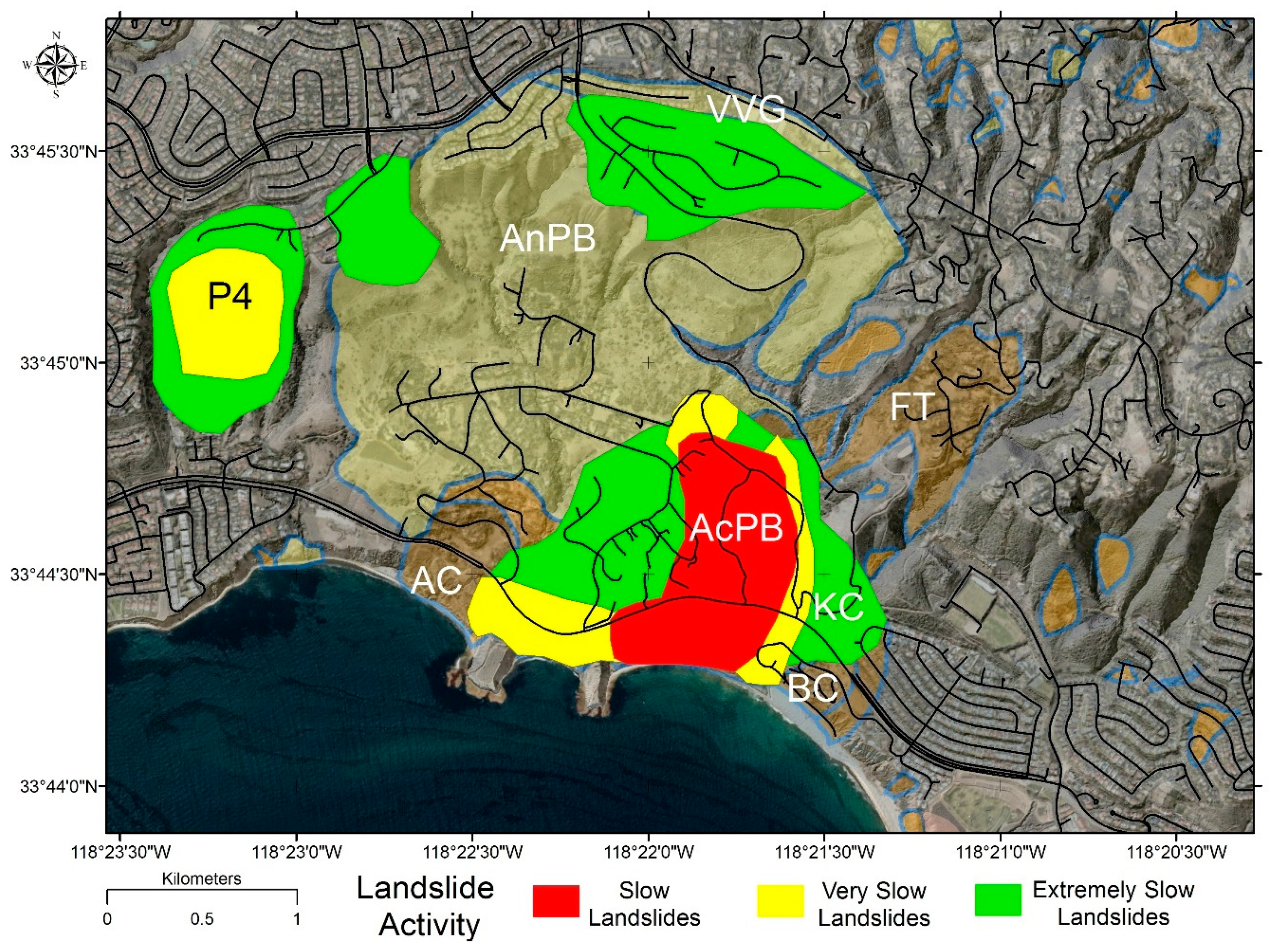
| Velocity Scale | Velocity Range | Description of Landslide Activity |
|---|---|---|
| Slow | >1.6 m/year | Fourteen GPS monuments experienced a velocity > 1.6 m/year for a portion of the study period. No location within the landslide complex moved at an average velocity > 1.6 m/year over the entire span of GPS or COSI-Corr observations. |
| Very Slow | 16 mm/year–1.6 m/year | Portions of the landslide complex that were consistently moving, as measured by COSI-Corr and GPS. There was typically a lack of PS presence in these areas since a velocity of 16 mm/year is near the maximum PS velocity threshold of 25 mm/year. |
| Extremely Slow | <16 mm/year | Velocity < 16 mm/year is below the accuracy of COSI-Corr and GPS measurements and, therefore, mapping of these areas relied exclusively on PSI results. |
| Stable | ~0 mm/year | Areas were considered stable if (1) COSI-Corr and GPS measurements were below the accuracy threshold and (2) PS with a velocity of ~0 mm/year were present. |
© 2019 by the authors. Licensee MDPI, Basel, Switzerland. This article is an open access article distributed under the terms and conditions of the Creative Commons Attribution (CC BY) license (http://creativecommons.org/licenses/by/4.0/).
Share and Cite
Bouali, E.H.; Oommen, T.; Escobar-Wolf, R. Evidence of Instability in Previously-Mapped Landslides as Measured Using GPS, Optical, and SAR Data between 2007 and 2017: A Case Study in the Portuguese Bend Landslide Complex, California. Remote Sens. 2019, 11, 937. https://doi.org/10.3390/rs11080937
Bouali EH, Oommen T, Escobar-Wolf R. Evidence of Instability in Previously-Mapped Landslides as Measured Using GPS, Optical, and SAR Data between 2007 and 2017: A Case Study in the Portuguese Bend Landslide Complex, California. Remote Sensing. 2019; 11(8):937. https://doi.org/10.3390/rs11080937
Chicago/Turabian StyleBouali, El Hachemi, Thomas Oommen, and Rüdiger Escobar-Wolf. 2019. "Evidence of Instability in Previously-Mapped Landslides as Measured Using GPS, Optical, and SAR Data between 2007 and 2017: A Case Study in the Portuguese Bend Landslide Complex, California" Remote Sensing 11, no. 8: 937. https://doi.org/10.3390/rs11080937